Bootstrap bandwidth selection for the pair correlation function of inhomogeneous spatial point processes

Abstract

This work focuses on kernel estimation of the pair correlation function (PCF) for inhomogeneous spatial point processes. We propose a bootstrap bandwidth selector based on minimizing the mean integrated squared error (MISE). The variance term is estimated by nonparametric bootstrap, and the bias by a plug-in approach using a pilot estimator of the PCF. Kernel estimators of the PCF also require a pilot estimator of the first-order intensity. We test the performance of the bandwidth selector and the role of the pilot intensity estimator in a simulation study. The bootstrap bandwidth selector is competitive with cross-validation procedures, but the contribution of the bandwidth parameter to the goodness-of-fit of the kernel PCF estimator is minor in comparison with that of the pilot intensity function. The data-based kernel intensity estimator leads to biased kernel PCF estimators, while both kernel and parametric covariate-based intensities provide accurate estimators of the PCF.

Keywords:

• Bandwidth selector
• kernel estimator: intensity function
• marked point bootstrap
• MISE
• pair correlation function

Mathematics Subject Classifications:

• 60G55
• 62G05
• 62F40

1. Introduction

A main interest in the analysis of spatial point processes is understanding and modelling the amount of interaction between events. Second-order properties such as Ripley´s K-function and the pair correlation function (PCF) have been widely used to characterize the dependence structure of spatial point processes [1–4]. The theory and estimation of these summary statistics have been mainly developed under stationarity, i.e. for spatial point processes with constant intensity function. Baddeley et al. [5] pointed out that this assumption can be very restrictive in practice and introduced second-order reweighted stationary (SOIRS) point processes as those with non-constant intensity function and translation invariant second-order characteristics, and second-order reweighted isotropic (SOIRI) point processes as those with isotropic second-order characteristics. They defined the inhomogeneous K-function of SOIRS and SOIRI point processes as extensions of Ripley´s K-function, and proposed nonparametric estimators for the inhomogeneous K-function and pair correlation functions.

Kernel smoothing is the main nonparametric estimator for the pair correlation function. As for any smoothing procedure, the statistical properties of the kernel estimator of the pair correlation function are highly dependent on the bandwidth parameter. Several data-driven procedures have been developed for stationary point processes, including fixed [6] and adaptive [7] rule of thumb, composite likelihood cross-validation [8], a semiparametric bootstrap procedure [9], and an AMSE-based adaptive plug-in bandwidth selector [10]. However, there are no evidences about the validity of these methods when dealing with inhomogeneous point processes. Guan [11] proposed a least squares cross-validation bandwidth selector for SOIRS point processes, which was adapted by Jalilian and Waagepetersen [12] to improve its computational efficiency.

In addition to bandwidth selection, kernel estimation of the pair correlation function requires an estimator of the first-order intensity function, if it is unknown. In the stationary framework, the consistency of the empirical intensity estimator guarantees the good performance of the kernel estimator of the pair correlation function. In the SOIRS framework, as pointed out by Diggle et al. [13], we can not estimate simultaneously the first and second-order structure of an inhomogeneous point process from a single realization without any additional information, such as covariates or the specification of a parametric model.

In this work we propose a semiparametric bootstrap bandwidth selector for the kernel estimator of the pair correlation function of SOIRI point processes. This proposal is inspired on the bootstrap bandwidth selector introduced by Loh and Jang [9] for the two-point correlation function of homogeneous point processes. We have conducted a simulation study with two main aims: (a) analyse the role of the first-order intensity estimator on the performance of the kernel estimator of the pair correlation function, and (b) test the performance of the bootstrap bandwidth selector by comparison with the rule of thumb and cross-validation procedures currently available. The plan of this paper is the following. Section 2 provides some background on the pair correlation function and its kernel estimators for SOIRI and SOIRI point processes. In Section 3, we introduce the bootstrap bandwidth selector. Section 4 outlines the results of the simulation study. The paper ends with a discussion in Section 5.

2. Kernel estimator of the pair correlation function

Consider a spatial point process $\mathbf{X}$ observed on a bounded domain $W\subset {\mathbb{R}}^2$, and let $\left|B\right|$ and $N\left(B\right)$ denote the area and number of events observed in any Borel set $B\subset {\mathbb{R}}^2$. For any $k\ge 1$ we say that $\mathbf{X}$ has kth-order intensity function, ${\lambda }_k:({\mathbb{R}}^2{)}^k\to (0,\mathrm{\infty })$, if for any disjoint Borel sets, $B_1,\dots B_k$ $\begin{array}{r}\mathbb{E}[N\left(B_1\right),\dots ,N\left(B_k\right)]={\int }_{B_1}\cdots {\int }_{B_k}{\lambda }_k(x_1,\dots ,x_k)\mathrm{d}{x}_1\dots \mathrm{d}{x}_k<\mathrm{\infty }.\end{array}$Intuitively, ${\lambda }_k(x_1,\dots ,x_k)\left|B_1\right|,\dots ,\left|B_k\right|$ gives the probability of observing one event in each Borel set. In particular for k = 1 and k = 2, we have the first and second-order intensities of $\mathbf{X}$, which are also defined as follows [2] $\begin{array}{r}\lambda \left(x\right)=\underset{\left|\mathrm{d}x\right|\to 0}{lim}\frac{E\left[N\right(\mathrm{d}x\left)\right]}{\left|\mathrm{d}x\right|},\end{array}$which measures the expected number of events per unit area, and $\begin{array}{r}{\lambda }_2(x,y)=\underset{\left|\mathrm{d}x\right|,\left|\mathrm{d}y\right|\to 0}{lim}\frac{E\left[N\right(\mathrm{d}x\left)N\right(\mathrm{d}y\left)\right]}{\left|\mathrm{d}x\right|\left|\mathrm{d}y\right|}.\end{array}$The pair correlation function (PCF) is defined as the ratio between the second and first-order intensity functions (1) $\begin{array}{r}g(x,y)=\frac{{\lambda }_2(x,y)}{\lambda \left(x\right)\lambda \left(y\right)},\end{array}$(1) and measures how the occurrence of an event in x affects the intensity at location y. A stationary point process has constant intensity, $\lambda \left(x\right)=\lambda$, and its second-order intensity and pair correlation function depend on the distance between points ${\lambda }_2(x,y)={\lambda }_2(x-y)$ and $g(x,y)=g(x-y)$. For stationary and isotropic point processes ${\lambda }_2(x,y)={\lambda }_2(\Vert x-y\Vert )={\lambda }_2\left(r\right)$, and $g(x,y)=g\left(r\right)$ for any $r>0$. An inhomogeneous spatial point process with first-order intensity bounded away from 0 is second-order intensity reweighted stationary (SOIRS) if $g(x,y)=g(x-y)$, and it is second-order intensity reweighted isotropic (SOIRI) when $g(x,y)=g(\Vert x-y\Vert )$ [5].

A typical kernel estimator of the PCF for a SOIRS point process is (2) $\begin{array}{r}{\hat{g}}_b\left(t\right)=\sum \sum _{x,y\in \mathbf{X}}^{\ne }\frac{{\mathbf{k}}_b(t-x+y)}{D(x,y)\lambda \left(x\right)\lambda \left(y\right)},\end{array}$(2) where ${\mathbf{k}}_b\left(r\right)=b^{-2}\mathbf{k}\left(r/b\right)$ is a two-dimensional kernel function with scalar bandwidth parameter b, and $D(x,y)$ is the edge correction. Among the edge correctors proposed for second-order properties [1,3], in this work we use the translation factor $D(x,y)=\left|\right(W-x)\cap (W-y\left)\right|=|W\cap (W-x+y\left)\right|$. Under isotropy, i.e. for a SOIRI point process, expression (2(2) $\begin{array}{r}{\hat{g}}_b\left(t\right)=\sum \sum _{x,y\in \mathbf{X}}^{\ne }\frac{{\mathbf{k}}_b(t-x+y)}{D(x,y)\lambda \left(x\right)\lambda \left(y\right)},\end{array}$(2) ) reduces to (3) $\begin{array}{r}{\hat{g}}_b\left(r\right)=\frac{1}{2\pi }\sum \sum _{x,y\in \mathbf{X}}^{\ne }\frac{k_b(r-\Vert x-y\Vert )}{D(x,y)\lambda \left(x\right)\lambda \left(y\right)\Vert x-y\Vert },\end{array}$(3) where $k_b\left(r\right)=b^{-1}k\left(r/b\right)$ is a one-dimensional kernel function with bandwidth parameter b. Typical choices of k include the uniform kernel, $k\left(r\right)=I\left(\right|r|\le 1/2)$, recommended by Illian et al. [3] and the Epanechnikov kernel $\begin{array}{r}k\left(x\right)=\frac{3}{4}{(1-x^2)}_{+}I\left(\right|r|\le 1),\end{array}$where $I(\cdot )$ is the indicator function, and $(x{)}_{+}=max\{0,x\}$ being the latter the most widely used.

The kernel estimator of the PCF is computationally fast and has a good performance for any $r\ge b$, but the estimators in expressions (2(2) $\begin{array}{r}{\hat{g}}_b\left(t\right)=\sum \sum _{x,y\in \mathbf{X}}^{\ne }\frac{{\mathbf{k}}_b(t-x+y)}{D(x,y)\lambda \left(x\right)\lambda \left(y\right)},\end{array}$(2) )–(3(3) $\begin{array}{r}{\hat{g}}_b\left(r\right)=\frac{1}{2\pi }\sum \sum _{x,y\in \mathbf{X}}^{\ne }\frac{k_b(r-\Vert x-y\Vert )}{D(x,y)\lambda \left(x\right)\lambda \left(y\right)\Vert x-y\Vert },\end{array}$(3) ) have a large negative bias when r<b. To overcome this drawback, Guan [11] proposed a bias-corrected estimator which, for SOIRI point processes, is given by (4) $\begin{array}{r}{\hat{g}}_{c,b}\left(r\right)={\displaystyle \frac{{\hat{g}}_b\left(r\right)}{c_b\left(r\right)}};c_b\left(r\right)={\int }_{-1}^{r/b}k\left(t\right)\mathrm{d}t.\end{array}$(4) The denominator in (4(4) $\begin{array}{r}{\hat{g}}_{c,b}\left(r\right)={\displaystyle \frac{{\hat{g}}_b\left(r\right)}{c_b\left(r\right)}};c_b\left(r\right)={\int }_{-1}^{r/b}k\left(t\right)\mathrm{d}t.\end{array}$(4) ) is equal to 1 if $r\ge b$, thus ${\hat{g}}_{c,b}\left(r\right)={\hat{g}}_b\left(r\right)$, and smaller than 1 if 0<r<b. Using the second-order Campbell formula, a second-order Taylor expansion, and the symmetry of the kernel function, the bias of ${\hat{g}}_b\left(r\right)$ for $r\ge b$ is (5) $\begin{array}{r}B\left[{\hat{g}}_b\left(r\right)\right]=\frac{b^2}{2}{g}^{\mathrm{\prime }\mathrm{\prime }}\left(r\right){\int }_{-1}^1{t}^{2}k\left(t\right)\mathrm{d}t+O\left(b^4\right),\end{array}$(5) which tends to 0 as $b\to 0$, if $g^{\mathrm{\prime }\mathrm{\prime }}\left(r\right)$ is bounded. In particular, ${\hat{g}}_b\left(r\right)$ is unbiased for Poisson point processes, as in this case $g\left(r\right)=1$.

On the other hand, for r<b we have (6) $\begin{array}{r}B\left[{\hat{g}}_{c,b}\left(r\right)\right]=c_b{\left(r\right)}^{-1}[-b{g}^{\mathrm{\prime }}(r\left){\int }_{-1}^{r/b}tk\right(t)\mathrm{d}t+\frac{b^2}{2}{g}^{\mathrm{\prime }\mathrm{\prime }}(r\left){\int }_{-1}^{r/b}{t}^{2}k\right(t)\mathrm{d}t+O\left(b^3\right)],\end{array}$(6) which, as in (5(5) $\begin{array}{r}B\left[{\hat{g}}_b\left(r\right)\right]=\frac{b^2}{2}{g}^{\mathrm{\prime }\mathrm{\prime }}\left(r\right){\int }_{-1}^1{t}^{2}k\left(t\right)\mathrm{d}t+O\left(b^4\right),\end{array}$(5) ), tends to 0 as $b\to 0$, if $g^{\mathrm{\prime }}\left(r\right)$ and $g^{\mathrm{\prime }\mathrm{\prime }}\left(r\right)$ are bounded. Therefore, ${\hat{g}}_{c,b}\left(r\right)$ is asymptotically unbiased for all r>0 (see details in Appendix A.1).

Using second to fourth order Campbell formulas, Taylor expansions, and ignoring higher-order interactions, as done by Stoyan and Stoyan [6] for homogeneous point processes (see details in Appendix A.2), the variance of the kernel PCF for any $r\ge b$ is (7) $\begin{array}{rl}\mathbb{V}ar\left[{\hat{g}}_b\left(r\right)\right]& ={\displaystyle \frac{1}{2{\pi }^2}}{\int }_{\Vert u\Vert <r+b}{\displaystyle \frac{k^2\left((r-\Vert u\Vert )/b\right)G_W^{\left(2\right)}\left(u\right)}{\Vert u{\Vert }^2{b}^2}}g(\Vert u\Vert )\mathrm{d}u\\ & ={\displaystyle \frac{1}{b\pi }}{\int }_{-1}^1{\displaystyle \frac{k^2\left(t\right)G_W^{\left(2\right)}(r-bt)}{(r-bt)}}g(r-bt)\mathrm{d}t,\end{array}$(7) and for r<b we have (8) $\begin{array}{rl}\mathbb{V}ar\left[{\hat{g}}_{c,b}\left(r\right)\right]& ={\displaystyle \frac{1}{2{\pi }^2{c}_b(r{)}^2}}{\int }_{\Vert u\Vert <r+b}{\displaystyle \frac{k^2\left((r-\Vert u\Vert )/b\right)G_W^{\left(2\right)}\left(u\right)}{\Vert u{\Vert }^2{b}^2}}g(\Vert u\Vert )\mathrm{d}u\\ & ={\displaystyle \frac{1}{b\pi c_b(r{)}^2}}{\int }_{-1}^{r/b}{\displaystyle \frac{k^2\left(t\right)G_W^{\left(2\right)}(r-bt)}{(r-bt)}}g(r-bt)\mathrm{d}t.\end{array}$(8) Due to the term $(r-bt)$ in the denominator of the right hand side of expression (7(7) $\begin{array}{rl}\mathbb{V}ar\left[{\hat{g}}_b\left(r\right)\right]& ={\displaystyle \frac{1}{2{\pi }^2}}{\int }_{\Vert u\Vert <r+b}{\displaystyle \frac{k^2\left((r-\Vert u\Vert )/b\right)G_W^{\left(2\right)}\left(u\right)}{\Vert u{\Vert }^2{b}^2}}g(\Vert u\Vert )\mathrm{d}u\\ & ={\displaystyle \frac{1}{b\pi }}{\int }_{-1}^1{\displaystyle \frac{k^2\left(t\right)G_W^{\left(2\right)}(r-bt)}{(r-bt)}}g(r-bt)\mathrm{d}t,\end{array}$(7) ), the variance increases as $r\to 0$. On the other hand, if the first-order intensity is bounded, $\lambda \left(x\right)<{\lambda }_{max}$, for some ${\lambda }_{max}>0$, then $G_W^2\left(u\right)\ge 1/\left(\right|W\cap W_u\left|{\lambda }_{max}\right)$, which tends to ∞ as r tends to the diameter of W. Therefore we need to establish an upper limit, $r_{max}$, up to which we estimate the pair correlation function. Given that in most cases interaction between events acts at small scales, this restriction does not imply any limitation in practice.

3. Bootstrap bandwidth selector

As we can see in expressions (5(5) $\begin{array}{r}B\left[{\hat{g}}_b\left(r\right)\right]=\frac{b^2}{2}{g}^{\mathrm{\prime }\mathrm{\prime }}\left(r\right){\int }_{-1}^1{t}^{2}k\left(t\right)\mathrm{d}t+O\left(b^4\right),\end{array}$(5) )–(8(8) $\begin{array}{rl}\mathbb{V}ar\left[{\hat{g}}_{c,b}\left(r\right)\right]& ={\displaystyle \frac{1}{2{\pi }^2{c}_b(r{)}^2}}{\int }_{\Vert u\Vert <r+b}{\displaystyle \frac{k^2\left((r-\Vert u\Vert )/b\right)G_W^{\left(2\right)}\left(u\right)}{\Vert u{\Vert }^2{b}^2}}g(\Vert u\Vert )\mathrm{d}u\\ & ={\displaystyle \frac{1}{b\pi c_b(r{)}^2}}{\int }_{-1}^{r/b}{\displaystyle \frac{k^2\left(t\right)G_W^{\left(2\right)}(r-bt)}{(r-bt)}}g(r-bt)\mathrm{d}t.\end{array}$(8) ) the goodness-of-fit of the kernel PCF estimator depends on the bandwidth parameter, which has to balance the well known bias-variance trade-off. For this reason, a global error measure such as the weighted mean integrated squared error (9) $\begin{array}{r}MISE\left(b\right)={\int }_0^R\mathbb{E}{\left[{\hat{g}}_b\right(r)-g(r\left)\right]}^{2}w\left(r\right)\mathrm{d}r,\end{array}$(9) where $R=r_{max}$ is the upper lag, and $w\left(r\right)$ a weighting factor, was proposed as a risk function to select the optimal bandwidth for the kernel estimator of the pair correlation function [11,12]. Jang and Loh [10] used a closed-form expression of the asymptotic mean squared error (AMSE) to propose a plug-in adaptive bandwidth selector for the two point correlation function of homogeneous point processes.

Considering $w\left(r\right)=1$ in expression (9(9) $\begin{array}{r}MISE\left(b\right)={\int }_0^R\mathbb{E}{\left[{\hat{g}}_b\right(r)-g(r\left)\right]}^{2}w\left(r\right)\mathrm{d}r,\end{array}$(9) ), we obtain the asymptotic mean integrated squared error as follows (10) $\begin{array}{r}AMISE\left(B\right)={\int }_o^{b}AMS{E}_c(r,b)\mathrm{d}r+{\int }_b^{R}AMSE(r,b)\mathrm{d}r,\end{array}$(10) where AMSE and $AMS{E}_c$ refer to the asymptotic mean squared error and bias-corrected mean squared errors (details in Appendix A.3). Integration of expressions (5(5) $\begin{array}{r}B\left[{\hat{g}}_b\left(r\right)\right]=\frac{b^2}{2}{g}^{\mathrm{\prime }\mathrm{\prime }}\left(r\right){\int }_{-1}^1{t}^{2}k\left(t\right)\mathrm{d}t+O\left(b^4\right),\end{array}$(5) ) and (7(7) $\begin{array}{rl}\mathbb{V}ar\left[{\hat{g}}_b\left(r\right)\right]& ={\displaystyle \frac{1}{2{\pi }^2}}{\int }_{\Vert u\Vert <r+b}{\displaystyle \frac{k^2\left((r-\Vert u\Vert )/b\right)G_W^{\left(2\right)}\left(u\right)}{\Vert u{\Vert }^2{b}^2}}g(\Vert u\Vert )\mathrm{d}u\\ & ={\displaystyle \frac{1}{b\pi }}{\int }_{-1}^1{\displaystyle \frac{k^2\left(t\right)G_W^{\left(2\right)}(r-bt)}{(r-bt)}}g(r-bt)\mathrm{d}t,\end{array}$(7) ) yields the following expression for the second term in (10(10) $\begin{array}{r}AMISE\left(B\right)={\int }_o^{b}AMS{E}_c(r,b)\mathrm{d}r+{\int }_b^{R}AMSE(r,b)\mathrm{d}r,\end{array}$(10) ) (11) $\begin{array}{rl}{\int }_b^{R}AMSE(r,b)\mathrm{d}r& ={\int }_b^R\frac{b^4}{4}{\left(g\mathrm{\prime }\mathrm{\prime }\right(r\left){\mu }_2\right(k\left)\right)}^2\mathrm{d}r\\ & +{\displaystyle \frac{1}{b\pi }}{\int }_b^R{\int }_{-1}^1{\displaystyle \frac{k^2\left(t\right)G_W^{\left(2\right)}(r-bt)}{(r-bt)}}g(r-bt)\mathrm{d}t\mathrm{d}r,\end{array}$(11) but integration of $AMS{E}_C(r,b)$ does not provide a tractable closed-form expression for the bias-corrected AMISE when r<b. In addition to the complex expression of the bias-corrected AMISE, the potential development of a plug-in bandwidth selector based on the AMISE, as done by Jang and Loh [10] for homogeneous point processes, is also hindered by the need of pilot estimators of $g\left(r\right)$, $g^{\mathrm{\prime }\mathrm{\prime }}\left(r\right)$ and $\lambda \left(x\right)$.

Following the proposal of Loh and Jang [9] for the two point correlation function of stationary point processes, here we introduce a semiparametric bootstrap bandwidth selector for the kernel estimator of the pair correlation function of SOIRI point processes. We use the MISE in expression (9(9) $\begin{array}{r}MISE\left(b\right)={\int }_0^R\mathbb{E}{\left[{\hat{g}}_b\right(r)-g(r\left)\right]}^{2}w\left(r\right)\mathrm{d}r,\end{array}$(9) ) with $w\left(r\right)=1$ as criterion to select the bandwidth parameter, and decompose it into its bias and variance terms. The variance term is estimated by the marked point bootstrap algorithm [14,15] using random sampling [16] instead of block bootstrap as in Loh [15]. The bias term is estimated through a plug-in approach based on a parametric pilot model, given that the nonparametric bootstrap provides unbiased estimators of the pair correlation function. Therefore, the bandwidth parameter is selected by the following semiparametric bootstrap algorithm:

1. For a given bandwidth, b, compute the bias-corrected kernel estimator of the pair correlation function, ${\hat{g}}_{c,b}\left(r\right)$.

2. Generate J bootstrap resamples $g_{b,j}^{\ast }\left(r\right),j=1,\dots J$ of ${\hat{g}}_{c,b}\left(r\right)$ implementing the marked point bootstrap algorithm as follows:

   	(2.1)	mark each event, $\{{\mathbf{x}}_{\mathbf{i}}{\}}_{i=1}^N$, with the kernel estimator of the local PCF, $m_i={\hat{g}}_b(r,{\mathbf{x}}_{\mathbf{i}})$, i.e. its contribution to the kernel estimator of the PCF $\begin{array}{r}{\hat{g}}_b(r,{\mathbf{x}}_{\mathbf{i}})=\frac{1}{2\pi }\sum _{y\in \mathbf{X},y\ne {\mathbf{x}}_{\mathbf{i}}}\frac{k_b(r-\Vert {\mathbf{x}}_i-y\Vert )}{D({\mathbf{x}}_{\mathbf{i}},y)\lambda \left({\mathbf{x}}_{\mathbf{i}}\right)\lambda \left(y\right)\Vert {\mathbf{x}}_{\mathbf{i}}-y\Vert }.\end{array}$
   	(2.2)	Generate J independent resamples of size N by random sampling with replacement on $1,\dots ,N$, $\{i_{1,j},\dots ,i_{N,j}{\}}_{j=1}^J$, and define the jth bootstrap PCF as the mean of the corresponding local PCFs $\begin{array}{r}{g}_{b,j}^{\star }\left(r\right)=\frac{1}{c_b\left(r\right)N}\sum _{k=1}^N{\hat{g}}_b(r,{\mathbf{x}}_{{\mathbf{i}}_{\mathbf{k}\mathbf{,}\mathbf{j}}}).\end{array}$

3. Fit a parametric model to the observed pattern and compute the corresponding PCF estimator $\hat{g}(r;\hat{\theta })$

4. Compute the bootstrap MISE $\begin{array}{rl}MIS{E}^{\ast }\left(b\right)& ={\mathbb{E}}_{\ast }\left[{\int }_0^R{\left[g_b^{\ast }\right(r)-\hat{g}(r;\hat{\theta }\left)\right]}^2\mathrm{d}r\right]\\ & ={\int }_0^{R}Bia{s}_{\ast }^2\left[g_b^{\ast }\right(r\left)\right]\mathrm{d}r+{\int }_0^R\mathbb{V}a{r}_{\ast }\left[g_b^{\ast }\right(r\left)\mathrm{d}r\right],\end{array}$where $\mathbb{V}a{r}_{\ast }\left[g_b^{\ast }\right(r\left)\right]$ is the variance with respect to the sampling bootstrap distribution, and the bias can be estimated through two alternative procedures.

   1. Asymptotic bias: using the first and second-order derivatives of $\hat{g}(r;\hat{\theta })$ as plug-in functions in expressions (5(5) $\begin{array}{r}B\left[{\hat{g}}_b\left(r\right)\right]=\frac{b^2}{2}{g}^{\mathrm{\prime }\mathrm{\prime }}\left(r\right){\int }_{-1}^1{t}^{2}k\left(t\right)\mathrm{d}t+O\left(b^4\right),\end{array}$(5) ) and (6(6) $\begin{array}{r}B\left[{\hat{g}}_{c,b}\left(r\right)\right]=c_b{\left(r\right)}^{-1}[-b{g}^{\mathrm{\prime }}(r\left){\int }_{-1}^{r/b}tk\right(t)\mathrm{d}t+\frac{b^2}{2}{g}^{\mathrm{\prime }\mathrm{\prime }}(r\left){\int }_{-1}^{r/b}{t}^{2}k\right(t)\mathrm{d}t+O\left(b^3\right)],\end{array}$(6) ).

   2. Empirical bootstrap bias: $\begin{array}{r}Bia{s}_{\ast }\left[g_b^{\ast }\right(r\left)\right]={\overline{g}}_b^{\ast }\left(r\right)-\hat{g}(r;\hat{\theta }),\end{array}$where ${\overline{g}}_b^{\ast }\left(r\right)$ is the empirical mean of the J bootstrap pair correlation functions.

It should be noted that for inhomogeneous point processes we need to estimate the first-order intensity function prior to obtaining the kernel or parametric estimator of the pair correlation function. Therefore, we need to check in which extent the intensity estimator affects bandwidth selection and, consequently, the performance of the kernel estimator of the pair correlation function.

Parametric or nonparametric approaches can be used to estimate the intensity function. We may know or assume that the intensity belongs to certain parametric family, and estimate the unknown parameters by maximum pseudolikelihood [2,17]. However, unreliable estimates can be obtained if the assumed parametric model deviates from the true intensity function. For this reason, nonparametric approaches, such as the kernel intensity estimator with fixed [2,18] or adaptive bandwidth [19], should be used when the observed pattern is the only information available. Finally, a kernel estimator based on covariates can be used if the intensity function depends on some spatial covariates but the parametric relationship among them is unknown. A rule of thumb [16] and bootstrap [20] bandwidth selectors have been proposed for this estimator.

4. Simulation study

We have conducted a simulation study with two main aims: (i) to test whether the estimator of the first-order intensity affects the performance of the kernel estimator of the pair correlation function, and (ii) to check the performance of the bootstrap bandwidth selector proposed in this work by comparison with the rule of thumb [6], least squares cross-validation [11,12] and composite likelihood cross-validation [8] bandwidth selectors. For this purpose, we have simulated 500 realizations of inhomogeneous Poisson and clustered point processes in the unit square. We generated inhomogeneous Poisson point processes with $m=\int \lambda \left(x\right)\mathrm{d}x=200$ and first-order intensity defined by two models:

Model 1	Using the simulation study in [15] as reference, $\lambda \left(x\right)$ is a log-Gaussian intensity function with a Gaussian Random field as spatial covariate, see Figures 1 and 3(top).
Model 2	$\lambda \left(x\right)$ is a log-Gaussian intensity function with wave model $Z(x,y)=1-0.5\ast co{s}^2\left(5x\right)$ as spatial covariate [21], see Figures 2 and 3(bottom).

Figure 1. Model 1: Gaussian random field used as spatial covariate (left), first-order intensity function of the Poisson point process (center), and pair correlation function of the Thomas cluster point processes with parent points intensity proportional to $\lambda \left(x\right)$ and $\mu =5$.

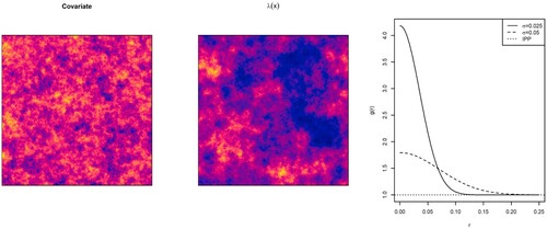
Figure 2. Model 2: Spatial covariate (left), first-order intensity function of the Poisson point process (center), and pair correlation function of the Thomas cluster point processes with parent points intensity proportional to $\lambda \left(x\right)$ and $\mu =5$.

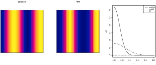
Figure 3. Poisson (left) and Thomas cluster point processes generated by Model 1 (top) and Model 2 (bottom).

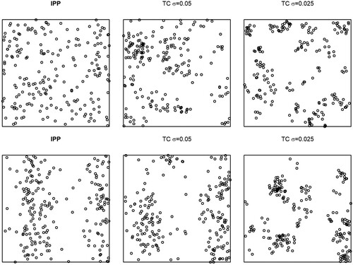
We generated Thomas Cluster point processes with $\sigma =0.05$ and $\sigma =0.025$ to generate different degrees of clustering and inhomogeneous parent points processes with $\kappa =40$ and first-order intensity proportional to those of the Poisson point processes Figures 1–3.

The simulation study was conducted with the aid of spatstat [22], ks [23] and RandomFields [24] packages of R [25].

4.1. Effect of the first-order intensity estimators

We have considered three different scenarios to analyse the effect of the first-order intensity estimator on the goodness-of-fit of the kernel estimator of the PCF. In particular, we consider the following three scenarios for the intensity estimation:

• Parametric intensity estimator with known covariate, estimated by maximum pseudolikelihood [17].

• Kernel intensity estimator with plug-in matrix bandwidth selector [18,26] and scalar adaptive bandwidth [27].

• Kernel intensity estimator based on a known spatial covariate with rule of thumb [16] and bootstrap [20] bandwidth.

For each realization of the point processes, we estimated the pair correlation function using the bias-corrected kernel estimator in expression (4(4) $\begin{array}{r}{\hat{g}}_{c,b}\left(r\right)={\displaystyle \frac{{\hat{g}}_b\left(r\right)}{c_b\left(r\right)}};c_b\left(r\right)={\int }_{-1}^{r/b}k\left(t\right)\mathrm{d}t.\end{array}$(4) ) using the three intensity estimators outlined above, and selecting the optimal bandwidth as that minimizing the empirical ISE (12) $\begin{array}{r}IS{E}_{\theta }\left(b\right)={\int }_0^R{\left[{\hat{g}}_b\right(r)-{\hat{g}}_{\hat{\theta }}(r\left)\right]}^2\mathrm{d}r\end{array}$(12) where ${\hat{g}}_{\hat{\theta }}\left(r\right)$ is the pilot parametric PCF estimator obtained using the same first-order intensity used in the kernel PCF. We have applied a Monte Carlo test based on the inhomogeneous L-function with B = 99 realizations of the null hypothesis to test the accuracy of the intensity estimators and the ISE (13) $\begin{array}{r}ISE\left(b\right)={\int }_0^R{\left[{\hat{g}}_b\right(r)-g(r\left)\right]}^2\mathrm{d}r\end{array}$(13) where $g\left(r\right)$ is the theoretical PCF, as discrepancy measure to compare the kernel PCF estimators.

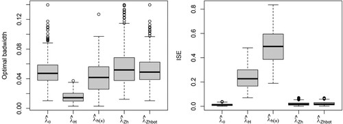
Figure 4 shows the first-order intensity estimators and the inhomogeneous L-tests for the Poisson point processes generated by Model 1. Comparison between the target (Figure 1, center) and the intensity estimators shows that the parametric and covariate-based kernel estimators provide accurate estimators of $\lambda \left(x\right)$, whereas the data-based kernel estimator with both fixed and adaptive bandwidth tends to oversmooth the intensity function. The inhomogeneous L-test shows that the five intensity estimators capture the second-order structure of the IPP. Figure 5(left) shows that, as expected, given that the theoretical PCF is constant, the optimal bandwidth tends to the upper limit of the selection interval. Although similar bandwidth parameters were obtained with the five intensity estimators, comparison between the ISEs Figure 5(right) shows that the kernel PCFs with covariate-based estimators and adaptive data-based kernel estimator perform better than that with the raw kernel intensity estimator with plug-in bandwidth matrix. PCF estimators with parametric and covariate-based kernel estimator with rule-of-thumbs outperformed those with data-based kernel estimator and covariate-based kernel with bootstrap bandwidth for Model 2 Figures 6 and 7. In fact, deviations from the Poisson model were detected at large distances when using the raw and covarate-based kernel intensity estimators with bootstrap bandwidth, whereas the rule of thumbs covariate-based estimators reported a better performance. Figures 8–11 and 12–15 show the intensity estimators and inhomogeneous L-test for the Thomas cluster point processes with parent point processes generated by Model 1 and 2, respectively. The parametric and covariate-based kernel estimators capture the first and second-order structures of the simulated patterns for the four point processes considered. The data-based kernel estimators, with both fixed and adaptive bandwidth, show a bias towards undersmoothing the intensity function, $\lambda \left(x\right)$, as these approaches interpret the positive interaction between events as hetereogeneity. Consequently, as shown in the inhomogeneous L-tests, we obtain negatively biased kernel estimators of the PCF with larger bias and ISE for clustered point processes with $\sigma =0.025$.

Figure 4. Model 1: First-order intensity estimators (top), parametric estimator (${\hat{\lambda }}_{\theta }$), kernel smoothing with plug-in bandwidth matrix (${\hat{\lambda }}_H$) and adaptive scalar bandwidth (${\hat{\lambda }}_{h\left(x\right)}$), covariate-based kernel estimator with rule of thumb (${\hat{\lambda }}_{Zh}$), and bootstrap bandwidth (${\hat{\lambda }}_{Zhboot}$). Inhomogeneous L-test for the Poisson point processes (bottom), confidence envelope (grey), mean inhomogeneous L-function of the null hypothesis (red), and inhomogeneous L-functon of the observed pattern.

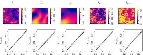
Figure 5. Model 1: Optimal bandwidth (left) and ISE (right) with parametric (${\hat{\lambda }}_{\theta }$), kernel with plug-in bandwidth matrix (${\hat{\lambda }}_H$) and adaptive scalar bandwidth (${\hat{\lambda }}_{h\left(x\right)}$), covariate-based kernel with rule of thumb (${\hat{\lambda }}_{Zh}$), and bootstrap bandwidth (${\hat{\lambda }}_{Zhboot}$) intensity estimators for Poisson point processes.

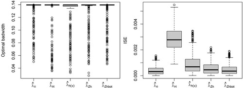
Figure 6. Model 2: First-order intensity estimators (top), and 1nhomogeneous L-test for the Poisson point processes (bottom), confidence envelope (grey), mean inhomogeneous L-function of the null hypothesis (red), and inhomogeneous L-functon of the observed pattern. See details in the caption of Figure 4.

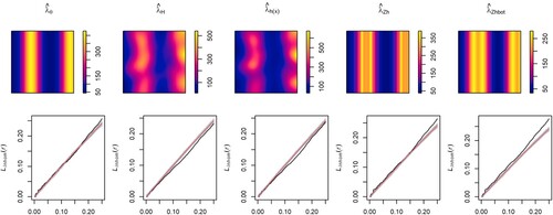
Figure 7. Model 2: Optimal bandwidth (left) and ISE (right) with parametric (${\hat{\lambda }}_{\theta }$), kernel (${\hat{\lambda }}_H$), covariate-based kernel with rule of thumb (${\hat{\lambda }}_{Zh}$), and bootstrap bandwidth (${\hat{\lambda }}_{Zhboot}$) intensity estimators for Poisson point processes.

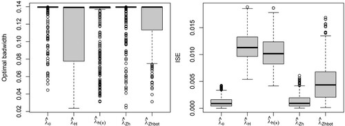
Figure 8. Model 1: First-order intensity estimators (top), and 1nhomogeneous L-test for Thomas cluster point processes with $\mu =5$ and $\sigma =0.05$ (bottom). See details in the caption of Figure 4.

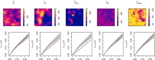
Figure 9. Model 1: Optimal bandwidth (left) and ISE (right) with parametric (${\hat{\lambda }}_{\theta }$), kernel (${\hat{\lambda }}_H$), covariate-based kernel with rule of thumb (${\hat{\lambda }}_{Zh}$), and bootstrap bandwidth (${\hat{\lambda }}_{Zhboot}$) intensity estimators Thomas cluster point processes with $\mu =5$ and $\sigma =0.05$.

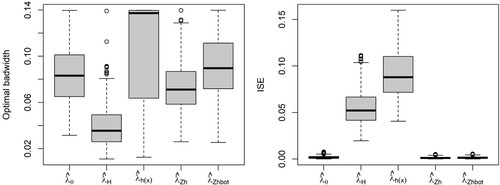
Figure 10. Model 1: First-order intensity estimators (top), and 1nhomogeneous L-test for Thomas cluster point processes with $\mu =5$ and $\sigma =0.025$ (bottom). See details in the caption of Figure 4.

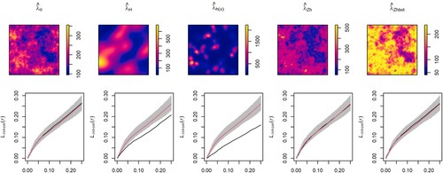
Figure 11. Model 1: Optimal bandwidth (left) and ISE (right) with parametric (${\hat{\lambda }}_{\theta }$), kernel (${\hat{\lambda }}_H$), covariate-based kernel with rule of thumb (${\hat{\lambda }}_{Zh}$), and bootstrap bandwidth (${\hat{\lambda }}_{Zhboot}$) intensity estimators Thomas cluster point processes with $\mu =5$ and $\sigma =0.025$.

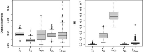
Figure 12. Model 2: First-order intensity estimators (top), and 1nhomogeneous L-test for Thomas cluster point processes with $\mu =5$ and $\sigma =0.05$ (bottom). See details in the caption of Figure 4.

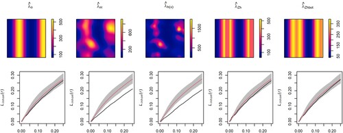
Figure 13. Model 2: Optimal bandwidth (left) and ISE (right) with parametric (${\hat{\lambda }}_{\theta }$), kernel (${\hat{\lambda }}_H$), covariate-based kernel with rule of thumb (${\hat{\lambda }}_{Zh}$), and bootstrap bandwidth (${\hat{\lambda }}_{Zhboot}$) intensity estimators Thomas cluster point processes with $\mu =5$ and $\sigma =0.05$.

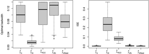
Figure 14. Model 2: First-order intensity estimators (top), and 1nhomogeneous L-test for Thomas cluster point processes with $\mu =5$ and $\sigma =0.025$ (bottom). See details in the caption of Figure 4.

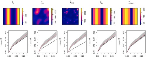
Figure 15. Model 2: Optimal bandwidth (left) and ISE (right) with parametric (${\hat{\lambda }}_{\theta }$), kernel (${\hat{\lambda }}_H$), covariate-based kernel with rule of thumb (${\hat{\lambda }}_{Zh}$), and bootstrap bandwidth (${\hat{\lambda }}_{Zhboot}$) intensity estimators Thomas cluster point processes with $\mu =5$ and $\sigma =0.025$.

4.2. Comparison of bandwidth selectors

In the second stage of the simulation study we focus on testing the performance of the semiparametric bandwidth selector with asymptotic (ABOOT) and empirical (EBOOT) bias. For this purpose, we have applied both bandwidth selectors to the simulated patterns with J = 200 using the five intensity estimators tested in Section 4.1. Finally, we considered the Thomas Cluster model, used to generate the simulated patterns, and a Matérn cluster model to analyse the role of the parametric pilot model needed to estimate the bias in the bootstrap algorithm.

In addition to comparing the two bootstrap algorithms proposed in this work, we have also compared the bootstrap bandwidth selector with the rule of thumb [6], the composite likelihood (CLCV, [8]) and least squares (LSCV, [11]) cross-validation bandwidth selectors currently available in the spatatst package of R [22]. The cross-validation bandwidth selectors use the bias-corrected PCF estimator in (4(4) $\begin{array}{r}{\hat{g}}_{c,b}\left(r\right)={\displaystyle \frac{{\hat{g}}_b\left(r\right)}{c_b\left(r\right)}};c_b\left(r\right)={\int }_{-1}^{r/b}k\left(t\right)\mathrm{d}t.\end{array}$(4) ), and the LSCV selector incorporates the fast algorithm by Jalilian and Waagepetersen [12]. As above, we use the ISE (expression (13(13) $\begin{array}{r}ISE\left(b\right)={\int }_0^R{\left[{\hat{g}}_b\right(r)-g(r\left)\right]}^2\mathrm{d}r\end{array}$(13) )) to compare the goodness-of-fit of the kernel PCF estimators.

Tables 1 and 2 outline the mean optimal bandwidth (b${}_{opt}$) and MISE of the kernel PCF estimators obtained for the different models, intensity estimators and bandwidth selectors tested in this work. As expected, in view of the results obtained in Section 4.1, the PCF estimator with raw kernel intensity estimators have a poor performance in comparison with those with covariate-based intensity estimators, mainly for the clustered point processes with adaptive bandwidth. Therefore, in advance we focus on the PCF estimators with covariate-based intensity estimators to compare the bandwidth selectors. It should also be noted that the rule of thumb, whose optimal bandwidth depends just on the expected number of events, provides the same optimal bandwidth regardless of the structure of the spatial point process and first-order intensity estimator used. The kernel PCF estimators obtained with this bandwidth tend to undersmooth the target PCF and have the largest ISE, with larger bias and variance than the remainder criteria, in particular at small distances ($r\to 0$) (see details in Figures 16–27).

For Poisson point processes, the cross-validation and bootstrap bandwidth selector provide large optimal bandwidths, as expected for a constant theoretical PCF, although the cross-validation bandwidths have larger variability than the bootstrap ones and tend to underestimate the optimal bandwidth. As a consequence, the ISE of kernel PCF estimators with cross-validation bandwidth are larger than those with bootstrap bandwidth Figures 16 and 18. Comparison between the bootstrap procedures does not report significant differences between using the asymptotic or empirical bias, or any effect of the wrong parametric model (MC) on the performance of the bandwidth selector Figures 16–19.

Figure 16. Model 1, IPP: Optimal bandwidth and MISE of the kernel PCF. Theoretical bandwidth (ISE${}_{o}pt$), Stoyan, least-squares (LSCV) and composite likelihood (CLIK) cross-validation, and bootstrap bandwidth selector with asymptotic (BOOT) and empirical (EBOOT) bias with Thomas cluster and Matérn (BOOT${}_{m}c$, EBOOT${}_{m}c$) pilot models, for parametric and covariate-based kernel intensity estimators.

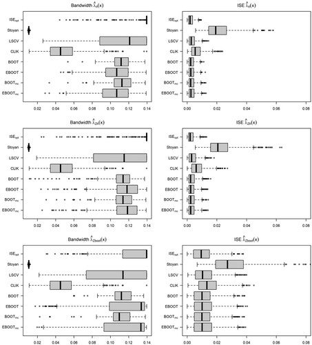
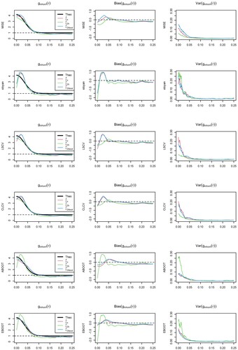
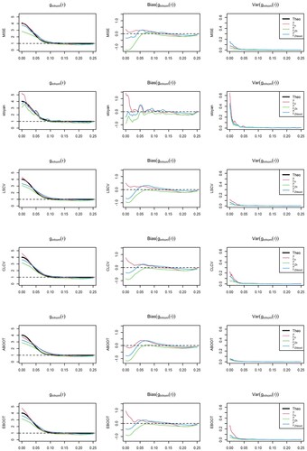
Figure 17. Model 1, IPP: Nonparametric pair correlation function (left), bias and variance of the estimators for the different bandwidth selectors and intensity estimators considered.

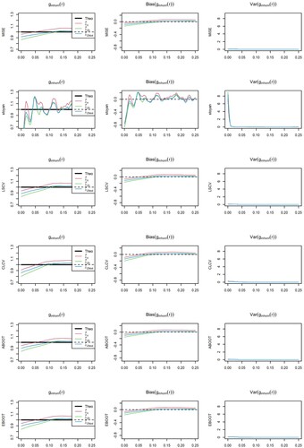
Figure 18. Model 2, IPP: Optimal bandwidth and MISE of the kernel PCF. Theoretical bandwidth (ISE${}_{o}pt$), Stoyan, least-squares (LSCV) and composite likelihood (CLIK) cross-validation, and bootstrap bandwidth selector with asymptotic (BOOT) and empirical (EBOOT) bias with Thomas cluster and Matérn (BOOT${}_{m}c$, EBOOT${}_{m}c$) pilot models, for parametric and covariate-based kernel intensity estimators.

Figure 19. Model 2, IPP: Nonparametric pair correlation function (left), bias and variance of the estimators for the different bandwidth selectors and intensity estimators considered.

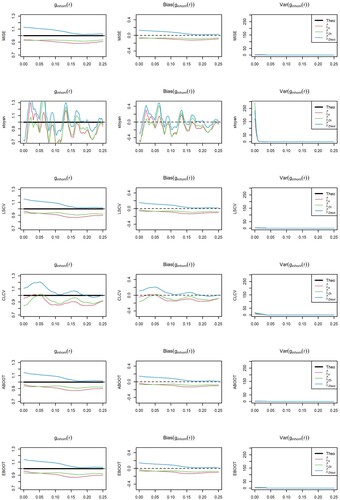
Table 1. Model 1: Optimal bandwidth ($b_{opt}$) and MISE of the kernel PCF.

					CV		BOOT		BOOT MC
			ISE${}_{opt}$	stoyan	LSCV	CLCV	ABOOT	EBOOT	ABOOT	EBOOT
IPP	${\lambda }_{\hat{\theta }}\left(x\right)$	$b_{opt}$	0.1316	0.0106	0.1077	0.0819	0.1133	0.1086	0.1113	0.1045
		MISE	0.0004	0.0033	0.0006	0.0007	0.0005	0.0005	0.0006	0.0006
	${\hat{\lambda }}_H\left(x\right)$	$b_{opt}$	0.1314	0.0106	0.1095	0.0821	0.1141	0.0943	0.1151	0.0937
		MISE	0.0029	0.0055	0.0031	0.0033	0.0030	0.0030	0.0030	0.0030
	${\hat{\lambda }}_{h\left(x\right)}\left(x\right)$	$b_{opt}$	0.1396	0.0106	0.109	0.0815	0.1142	0.109	0.1141	0.1067
		MISE	0.0007	0.0033	0.0009	0.0009	0.0007	0.0007	0.0007	0.0008
	${\hat{\lambda }}_{cov,rt}\left(x\right)$	$b_{opt}$	0.1293	0.0106	0.1064	0.0810	0.1133	0.1065	0.1133	0.1045
		MISE	0.0006	0.0035	0.0007	0.0009	0.0006	0.0006	0.0006	0.0006
	${\hat{\lambda }}_{Z,boot}\left(x\right)$	$b_{opt}$	0.1308	0.0106	0.1053	0.0811	0.1137	0.1104	0.1122	0.1092
		MISE	0.0005	0.0035	0.0007	0.0008	0.0005	0.0005	0.0005	0.0005
TC	${\lambda }_{\hat{\theta }}\left(x\right)$	$b_{opt}$	0.0882	0.0106	0.0582	0.0453	0.1057	0.0818	0.0948	0.0728
$\sigma =0.05$		MISE	0.0017	0.0061	0.0024	0.0027	0.0022	0.0019	0.0021	0.0019
	${\hat{\lambda }}_H\left(x\right)$	$b_{opt}$	0.0451	0.0106	0.0494	0.0457	0.1084	0.0973	0.1046	0.0940
		MISE	0.0029	0.0518	0.0499	0.0499	0.0519	0.0517	0.0518	0.0516
	${\hat{\lambda }}_{h\left(x\right)}\left(x\right)$	$b_{opt}$	0.1047	0.0107	0.0995	0.044	0.0895	0.0565	0.1123	0.0711
		MISE	0.0931	0.0982	0.0943	0.0957	0.0946	0.0949	0.0941	0.0948
	${\hat{\lambda }}_{cov,rt}\left(x\right)$	$b_{opt}$	0.0796	0.0105	0.0575	0.0456	0.1052	0.0748	0.0959	0.0709
		MISE	0.0018	0.0052	0.0017	0.0019	0.0017	0.0013	0.0015	0.0013
	${\hat{\lambda }}_{Z,boot}\left(x\right)$	$b_{opt}$	0.0878	0.0106	0.0543	0.0452	0.1038	0.0779	0.0927	0.0692
		MISE	0.0024	0.0169	0.0124	0.0130	0.0121	0.0111	0.0119	0.0114
TC	${\lambda }_{\hat{\theta }}\left(x\right)$	$b_{opt}$	0.0357	0.0107	0.0262	0.0319	0.0551	0.0395	0.0398	0.0337
$\sigma =0.025$		MISE	0.0069	0.0175	0.0098	0.0084	0.0128	0.0078	0.0086	0.0074
	${\hat{\lambda }}_H\left(x\right)$	$b_{opt}$	0.0162	0.0107	0.0268	0.0319	0.0443	0.0277	0.0341	0.0259
		MISE	0.1458	0.1489	0.1504	0.1520	0.1603	0.1505	0.1532	0.1497
	${\hat{\lambda }}_{h\left(x\right)}\left(x\right)$	$b_{opt}$	0.0340	0.0107	0.0403	0.0319	0.0296	0.0306	0.1075	0.0359
		MISE	0.4889	0.4917	0.4928	0.4909	0.4913	0.4901	0.5009	0.4902
	${\hat{\lambda }}_{cov,rt}\left(x\right)$	$b_{opt}$	0.0331	0.0107	0.0268	0.0319	0.0532	0.0357	0.0406	0.0323
		MISE	0.0050	0.0124	0.0066	0.0061	0.0107	0.0056	0.0070	0.0058
	${\hat{\lambda }}_{Z,boot}\left(x\right)$	$b_{opt}$	0.0374	0.0107	0.0272	0.0320	0.0540	0.0401	0.0405	0.0354
		MISE	0.0060	0.0161	0.0086	0.0076	0.0104	0.0067	0.0076	0.0069

Notes: Empirical optimal bandwidth (ISE${}_{opt}$), Stoyan, least-squares (LSCV) and composite likelihood (CLCV) cross-validation, and bootstrap bandwidth selector, with Thomas cluster (TC) and Matérn (MC) pilot models, under the five scenarios considered for the first-order intensity.

Table 2. Model 2: Optimal bandwidth ($b_{opt}$) and MISE of the kernel PCF.

					CV		BOOT		BOOT MC
			ISE${}_{opt}$	stoyan	LSCV	CLCV	ABOOT	EBOOT	ABOOT	EBOOT
IPP	${\lambda }_{\hat{\theta }}\left(x\right)$	$b_{opt}$	0.1396	0.0106	0.1209	0.0453	0.1116	0.1068	0.1125	0.1068
		MISE	0.0009	0.0086	0.0012	0.0024	0.0011	0.0011	0.0011	0.0011
	${\hat{\lambda }}_H\left(x\right)$	$b_{opt}$	0.1380	0.0106	0.1396	0.0449	0.1140	0.0892	0.1148	0.0886
		MISE	0.0112	0.0137	0.0114	0.0120	0.0113	0.0114	0.0113	0.0114
	${\hat{\lambda }}_{h\left(x\right)}\left(x\right)$	$b_{opt}$	0.1396	0.0106	0.109	0.0815	0.1142	0.109	0.1141	0.1067
		MISE	0.0007	0.0033	0.0009	0.0009	0.0007	0.0007	0.0007	0.0008
	${\hat{\lambda }}_{cov,rt}\left(x\right)$	$b_{opt}$	0.1396	0.0106	0.1149	0.0453	0.1138	0.1181	0.1137	0.1187
		MISE	0.0009	0.0092	0.0013	0.0027	0.0010	0.0011	0.0011	0.0011
	${\hat{\lambda }}_{Z,boot}\left(x\right)$	$b_{opt}$	0.1396	0.0106	0.1137	0.0452	0.1119	0.1336	0.1097	0.1333
		MISE	0.0042	0.0121	0.0046	0.0059	0.0045	0.0045	0.0045	0.0045
TC	${\lambda }_{\hat{\theta }}\left(x\right)$	$b_{opt}$	0.0996	0.0101	0.0653	0.0384	0.1000	0.0640	0.0844	0.0598
$\sigma =0.05$		MISE	0.0020	0.0138	0.0034	0.0050	0.0025	0.0030	0.0026	0.0032
	${\hat{\lambda }}_H\left(x\right)$	$b_{opt}$	0.0152	0.0099	0.0278	0.0318	0.0472	0.0282	0.0351	0.0274
		MISE	0.2440	0.2457	0.2491	0.2512	0.2599	0.2484	0.2520	0.2480
	${\hat{\lambda }}_{h\left(x\right)}\left(x\right)$	$b_{opt}$	0.1047	0.0107	0.0995	0.044	0.0895	0.0565	0.1123	0.0711
		MISE	0.0931	0.0982	0.0943	0.0957	0.0946	0.0949	0.0941	0.0948
	${\hat{\lambda }}_{cov,rt}\left(x\right)$	$b_{opt}$	0.1007	0.0090	0.0735	0.0338	0.0912	0.0733	0.0794	0.0745
		MISE	0.0043	0.0231	0.0068	0.0103	0.0052	0.0059	0.0057	0.0060
	${\hat{\lambda }}_{Z,boot}\left(x\right)$	$b_{opt}$	0.0796	0.0100	0.0622	0.0389	0.1015	0.0606	0.0842	0.0585
		MISE	0.0018	0.0114	0.0027	0.0038	0.0024	0.0024	0.0023	0.0024
TC	${\lambda }_{\hat{\theta }}\left(x\right)$	$b_{opt}$	0.0465	0.0099	0.0310	0.0321	0.0522	0.0314	0.0330	0.0289
$\sigma =0.025$		MISE	0.0103	0.0372	0.0150	0.0158	0.0124	0.0154	0.0133	0.0164
	${\hat{\lambda }}_H\left(x\right)$	$b_{opt}$	0.0143	0.0099	0.0261	0.0322	0.0443	0.0286	0.0340	0.0268
		MISE	0.2248	0.2267	0.2302	0.2332	0.2394	0.2314	0.2310	0.2287
	${\hat{\lambda }}_{h\left(x\right)}\left(x\right)$	$b_{opt}$	0.0409	0.0099	0.0502	0.0321	0.0280	0.0383	0.1062	0.0407
		MISE	0.4962	0.4990	0.5001	0.4996	0.4984	0.4973	0.5059	0.4970
	${\hat{\lambda }}_{cov,rt}\left(x\right)$	$b_{opt}$	0.0492	0.0099	0.0335	0.0319	0.0496	0.0324	0.0388	0.0348
		MISE	0.0164	0.0589	0.0254	0.0254	0.0197	0.0234	0.0213	0.0231
	${\hat{\lambda }}_{Z,boot}\left(x\right)$	$b_{opt}$	0.0487	0.0099	0.0316	0.0321	0.0523	0.0323	0.0336	0.0314
		MISE	0.0171	0.0555	0.0269	0.0288	0.0217	0.0237	0.0242	0.0244

Notes: Empirical optimal bandwidth (ISE${}_{opt}$), Stoyan, least-squares (LSCV) and composite likelihood (CLCV) cross-validation, and bootstrap bandwidth selector, with Thomas cluster (TC) and Matérn (MC) pilot models, under the five scenarios considered for the first-order intensity.

For Thomas cluster point processes with intensity defined by Model 1 Figures 20 – 23, all bandwidth selectors but the asymptotic bootstrap with Thomas cluster pilot model underestimate the optimal bandwidth, but this bias in the bandwidth selector does not affect the performance of the kernel PCF. In contrast, the bootstrap bandwidth selector with asymptotic bias (ABOOT) tend to overestimate the optimal bandwidth, resulting in a larger ISE in the most clustered point process, $\sigma =0.025$, whereas the bootstrap bandwidth selector with empirical bias (EBOOT) provides a good estimator of the optimal bandwidth. We have not found any negative impact of using a wrong parametric pilot model in the bootstrap bandwidth selector. Finally, Figures 21 and 23 show that the covariate-based kernel estimator with rule of thumb bandwidth performs slightly worse than that with bootstrap bandwidth and the parametric estimator.

Figure 20. Model 1, TC$(\mu =5,\sigma =0.05)$: Optimal bandwidth and MISE of the kernel PCF. Theoretical bandwidth (ISE${}_{o}pt$), Stoyan, least-squares (LSCV) and composite likelihood (CLIK) cross-validation, and bootstrap bandwidth selector with asymptotic (BOOT) and empirical (EBOOT) bias with Thomas cluster and Matérn (BOOT${}_{m}c$ and EBOOT${}_{m}c$) pilot models, for parametric and covariate-based kernel intensity estimators.

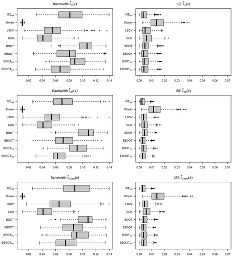
Figure 21. Model 1, TC$(\mu =5,\sigma =0.05)$: Nonparametric pair correlation function (left), bias and variance of the estimators for the different bandwidth selectors and intensity estimators considered.

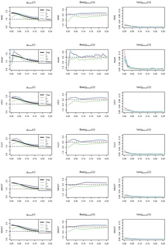
Figure 22. Model 1, TC$(\mu =5,\sigma =0.025)$: Optimal bandwidth and MISE of the kernel PCF. Theoretical bandwidth (ISE${}_{o}pt$), Stoyan, least-squares (LSCV) and composite likelihood (CLIK) cross-validation, and bootstrap bandwidth selector with asymptotic (BOOT) and empirical (EBOOT) bias with Thomas cluster and Matérn (BOOT${}_{m}c$ and EBOOT${}_{m}c$) pilot models, for parametric and covariate-based kernel intensity estimators.

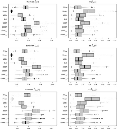
Figure 23. Model 1, TC$(\mu =5,\sigma =0.025)$: Nonparametric pair correlation function (left), bias and variance of the estimators for the different bandwidth selectors and intensity estimators considered.

For Thomas cluster point processes with intensity defined by Model 2 and $\sigma =0.05$ Figures 24 and 25, CLCV underestimates the optimal bandwidth and the bootstrap bandwidth selector with asymptotic bias (ABOOT) tends to overestimate the optimal bandwidth. For point processes with $\sigma =0.025$ Figures 26 and 27 all selector but the asymptotic bootstrap with Thomas cluster pilot model, which overestimates the optimal bandwidth, have a slight bias towards underestimating the target bandwidth. However, these biases in the optimal bandwidth have a minor impact on the goodness-of-fit of the kernel PCF estimator, as we do not observe differences between the respective ISEs. As observed for Model 1, PCF estimators with the rule of thumbs covariate-based kernel intensity estimator have larger ISE than those with bootstrap bandwidth in the covariate-based kernel and parametric intensity estimator, which have similar performance.

Figure 24. Model 2, TC$(\mu =5,\sigma =0.05)$: Optimal bandwidth and MISE of the kernel PCF. Theoretical bandwidth (ISE${}_{o}pt$), Stoyan, least-squares (LSCV) and composite likelihood (CLIK) cross-validation, and bootstrap bandwidth selector with asymptotic (BOOT) and empirical (EBOOT) bias with Thomas cluster and Matérn (BOOT${}_{m}c$ and EBOOT${}_{m}c$) pilot models, for parametric and covariate-based kernel intensity estimators.

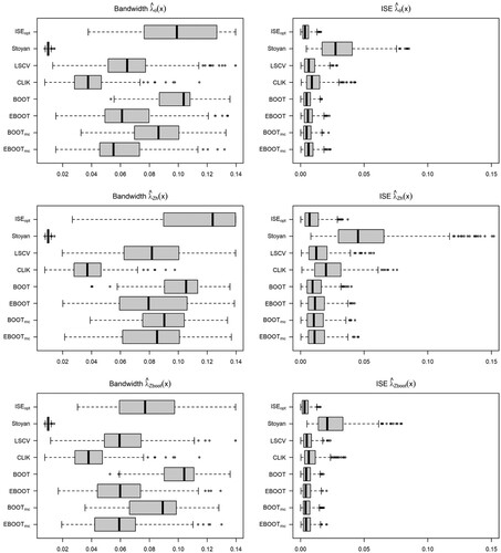
Figure 25. Model 2, TC$(\mu =5,\sigma =0.05)$: Nonparametric pair correlation function (left), bias and variance of the estimators for the different bandwidth selectors and intensity estimators considered.

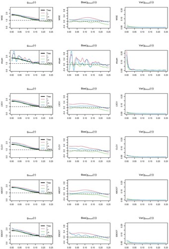
Figure 26. Model 2, TC$(\mu =5,\sigma =0.025)$: Optimal bandwidth and MISE of the kernel PCF. Theoretical bandwidth (ISE${}_{o}pt$), Stoyan, least-squares (LSCV) and composite likelihood (CLIK) cross-validation, and bootstrap bandwidth selector with asymptotic (BOOT) and empirical (EBOOT) bias with Thomas cluster and Matérn (BOOT${}_{m}c$ and EBOOT${}_{m}c$) pilot models, for parametric and covariate-based kernel intensity estimators.

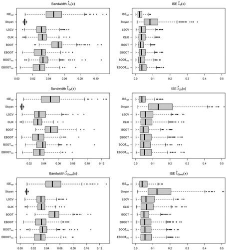
Figure 27. Model 2, TC$(\mu =5,\sigma =0.025)$: Nonparametric pair correlation function (left), bias and variance of the estimators for the different bandwidth selectors and intensity estimators considered.

5. Discussion

This work introduces a semiparametric bootstrap bandwidth selector for the kernel estimator of the pair correlation function of inhomogenoeus spatial point processes, which can be seen as an extension of the bootstrap bandwidth selector introduced by Loh and Jang [9] for the two points correlation function of homogeneous point processes. To implement this bandwidth selector we split the MISE of the kernel PCF estimator into its bias and variance terms. The bias is estimated by a plug-in procedure using a pilot parametric model for the PCF, and the variance is estimated through a marked point bootstap algorithm [14,15].

This procedure has larger computational cost than plug-in algorithms, such as the AMSE based selector in Jang and Loh [10] for homogeneous point processes. However, as argued in Section 3, the untractable AMISE expression for the bias-corrected kernel PCF estimator and the need of a pilot estimator of the first-order intensity, in addition to the pilot PCF function, do not allow the development of a plug-in estimator, in the inhomogeneous framework. On the other hand, the nonparametric bootstrap algorithm provides a consistent estimator of the variance but, as the bootstrap estimate of the PCF is unbiased [15], we cannot use a nonparametric algorithm.

The simulation study, in addition to testing the performance of the bandwidth selector, addresses a key problem in nonparametric estimation of second-order properties, the need of a pilot estimator of the first-order intensity. As expected, given that we cannot distinguish between heterogeneity and dependence in a single point pattern [2], kernel PCF estimators with a kernel intensity estimator have a large negative bias which increases with the degree of clustering of the simulated point processes. Notice that, in absence of additional information, the kernel intensity function interprets clustering as inhomogeneity providing an estimator of the conditional intensity instead of the first-order intensity. Kernel PCF estimators with parametric intensity estimator and kernel covariate-based intensity estimators have similar performance and, consequently, the latter may be a good choice in real data applications when the covariates driving the spatial distribution of events are known, but not the model that determines the relationship between covariate and events.

Focusing on the bootstrap bandwidth selector, we have seen that the assumption of a wrong pilot model in the bias component has a minor impact on the performance of the bandwidth selector. We have also seen that the asymptotic and empirical plug-in bias estimators provide similar results. The semiparametric bootstrap bandwidth selector outperforms the computationally efficient rule of thumbs [6], which estimates the optimal bandwidth as a function of the number of events. Our proposal is competitive with cross-validation algorithms, but none of them outperforms the other. In fact, even when different optimal bandwidths are obtained with the cross-validation and bootstrap selectors, these differences do not affect the goodness-of-fit of the kernel PCF estimator.

In summary, we have developed a semiparametric bootstrap bandwidth selector for the kernel PCF estimator which is competitive with cross-validation algorithms. We have seen that the bandwidth parameter has a minor impact on the goodness-of-fit of the kernel PCF estimator in comparison with the pilot intensity required to compute the estimator. Recently, Shaw et al. [21] proposed a globally intensity-weighted estimator of the PCF which reduces the bias of PCF estimator with data-based kernel intensity. Comparison of this new approach with those with covariate-based pilot intensity function and adaptation of the semiparametric bootstrap to this new approach would be useful contributions to this research line.

Disclosure statement

No potential conflict of interest was reported by the author(s).

Additional information

Funding

This work has been supported by the Agencia Estatal de Investigación (AEI)/FEDER, UE [project numbers MTM2016-76969-P, PID2019-107392RB-I00 and PID2020-116587GB-I00].

Appendix

Appendix 1

Performance of the kernel PCF estimator

The mean integrated squared error (MISE) is a common global error measure for the performance of a kernel estimator and, consequently, has been widely used as criterion to find a bandwidth parameter that balances the trade-off between bias and variance. In particular, a weighted mean integrated squared error (A1) $\begin{array}{r}MISE\left(b\right)={\int }_0^R\mathbb{E}{\left[{\hat{g}}_b\right(r)-g(r\left)\right]}^{2}w\left(r\right)\mathrm{d}r\end{array}$(A1) where $R=r_{max}$ is the upper lag, and $w\left(r\right)$ a weight factor, was proposed as a risk function to select the optimal bandwidth for the kernel estimator of the PCF [11,12]. In the same line as Guan [11] and Jalilian and Waagepetersen [12], this section analyses the bias and variance of the kernel PCF estimator and provides an expression for its AMISE.

A.1. Bias

The kth-order Campbell formula [4] states that for any Borel function $f:({\mathbb{R}}^2{)}^k\to [0,\mathrm{\infty })$ (A2) $\begin{array}{rl}& \mathbb{E}\left[\sum _{x_1,\dots ,x_k\in \mathbf{X}}^{\ne }f(x_1,\dots ,x_k)\right]=\int \dots \int f(x_1,\dots ,x_k){\lambda }_k(x_1,\dots ,x_k)\mathrm{d}{x}_1,\dots \mathrm{d}{x}_k\\ & =\int \dots \int f(x_1,\dots ,x_k)\left[\prod _{j=1}^k\lambda \right(x_j\left)\right]g_k(x_1,\dots ,x_k)\mathrm{d}{x}_1,\dots \mathrm{d}{x}_k<\mathrm{\infty }\end{array}$(A2) where $g_k(\cdot )$ is the kth-order normalized joint intensity. Thus, considering $\begin{array}{r}f(x,y)=\frac{I_W\left(x\right)I_W\left(y\right)k_b(r-\Vert x-y\Vert )}{|W\cap W_{x-y}|\lambda \left(x\right)\lambda \left(y\right)\Vert x-y\Vert }\end{array}$and using the second-order Campbell formula (k = 2 in (A2(A2) $\begin{array}{rl}& \mathbb{E}\left[\sum _{x_1,\dots ,x_k\in \mathbf{X}}^{\ne }f(x_1,\dots ,x_k)\right]=\int \dots \int f(x_1,\dots ,x_k){\lambda }_k(x_1,\dots ,x_k)\mathrm{d}{x}_1,\dots \mathrm{d}{x}_k\\ & =\int \dots \int f(x_1,\dots ,x_k)\left[\prod _{j=1}^k\lambda \right(x_j\left)\right]g_k(x_1,\dots ,x_k)\mathrm{d}{x}_1,\dots \mathrm{d}{x}_k<\mathrm{\infty }\end{array}$(A2) )), we can write the mean of the kernel PCF in (3(3) $\begin{array}{r}{\hat{g}}_b\left(r\right)=\frac{1}{2\pi }\sum \sum _{x,y\in \mathbf{X}}^{\ne }\frac{k_b(r-\Vert x-y\Vert )}{D(x,y)\lambda \left(x\right)\lambda \left(y\right)\Vert x-y\Vert },\end{array}$(3) ) for any $r\ge 0$ and b>0 as (A3) $\begin{array}{rl}\mathbb{E}\left[{\hat{g}}_b\left(r\right)\right]& =\frac{1}{2\pi }{\int }_{{\mathbb{R}}^2}{\int }_{\Vert u\Vert <r+b}\frac{I(x\in W\cap W_u)k_b(r-\Vert u\Vert )}{|W\cap W_u|\Vert u\Vert }g(\Vert u\Vert )\mathrm{d}u\mathrm{d}x\\ & ={\int }_{\Vert u\Vert <r+b}\frac{k\left((r-\Vert u\Vert )/b\right)}{b\Vert u\Vert }g(\Vert u\Vert )\mathrm{d}u={\int }_{-1}^{min\{1,r/b\}}k\left(t\right)g(r-bt)\mathrm{d}t\end{array}$(A3) Thus, $\begin{array}{r}\mathbb{E}\left[{\hat{g}}_b\left(r\right)\right]\approx g\left(r\right){\int }_{-1}^{r/b}k\left(t\right)\mathrm{d}t\le g\left(r\right){\int }_{-1}^{1}k\left(t\right)\mathrm{d}t=g\left(r\right)\end{array}$and, consequently, ${\hat{g}}_b\left(r\right)$ is asymptotically unbiased for $r\ge b$ and has a negative bias at small distances, i.e. for r<b. This drawback can be overcome using the bias-corrected estimator introduced by Guan [11] (A4) $\begin{array}{r}{\hat{g}}_{c,b}\left(r\right)={\displaystyle \frac{{\hat{g}}_b\left(r\right)}{c_b\left(r\right)}};c_b\left(r\right)={\int }_{-1}^{r/b}k\left(t\right)\mathrm{d}t\end{array}$(A4) The denominator in (A4(A4) $\begin{array}{r}{\hat{g}}_{c,b}\left(r\right)={\displaystyle \frac{{\hat{g}}_b\left(r\right)}{c_b\left(r\right)}};c_b\left(r\right)={\int }_{-1}^{r/b}k\left(t\right)\mathrm{d}t\end{array}$(A4) ) is equal to 1 if $r\ge b$, thus ${\hat{g}}_{c,b}\left(r\right)={\hat{g}}_b\left(r\right)$, and smaller than 1 if 0<r<b.

Going back to expression (A3(A3) $\begin{array}{rl}\mathbb{E}\left[{\hat{g}}_b\left(r\right)\right]& =\frac{1}{2\pi }{\int }_{{\mathbb{R}}^2}{\int }_{\Vert u\Vert <r+b}\frac{I(x\in W\cap W_u)k_b(r-\Vert u\Vert )}{|W\cap W_u|\Vert u\Vert }g(\Vert u\Vert )\mathrm{d}u\mathrm{d}x\\ & ={\int }_{\Vert u\Vert <r+b}\frac{k\left((r-\Vert u\Vert )/b\right)}{b\Vert u\Vert }g(\Vert u\Vert )\mathrm{d}u={\int }_{-1}^{min\{1,r/b\}}k\left(t\right)g(r-bt)\mathrm{d}t\end{array}$(A3) ), a second-order Taylor expansion yields $\begin{array}{r}\mathbb{E}\left[{\hat{g}}_b\left(r\right)\right]={\int }_{-1}^{min\{1,r/b\}}k\left(t\right)\left(g\right(r)-bt{g}^{\mathrm{\prime }}(r)+\frac{(bt{)}^2}{2}{g}^{\mathrm{\prime }\mathrm{\prime }}(r\left)\right)\mathrm{d}t\end{array}$Thus, given the symmetry of the kernel function, the bias of ${\hat{g}}_b\left(r\right)$ for $r\ge b$ is (A5) $\begin{array}{r}B\left[{\hat{g}}_b\left(r\right)\right]=\frac{b^2}{2}{g}^{\mathrm{\prime }\mathrm{\prime }}\left(r\right){\int }_{-1}^1{t}^{2}k\left(t\right)\mathrm{d}t+O\left(b^4\right)\end{array}$(A5) which tends to 0 as $b\to 0$, if $g^{\mathrm{\prime }\mathrm{\prime }}\left(r\right)$ is bounded. In particular, ${\hat{g}}_b\left(r\right)$ is unbiased for Poisson point processes, as in this case $g\left(r\right)=1$.

On the other hand, for r<b we have (A6) $\begin{array}{r}B\left[{\hat{g}}_{c,b}\left(r\right)\right]=c_b{\left(r\right)}^{-1}[-b{g}^{\mathrm{\prime }}(r\left){\int }_{-1}^{r/b}tk\right(t)\mathrm{d}t+\frac{b^2}{2}{g}^{\mathrm{\prime }\mathrm{\prime }}(r\left){\int }_{-1}^{r/b}{t}^{2}k\right(t)\mathrm{d}t+O\left(b^3\right)]\end{array}$(A6) which, as in (A5(A5) $\begin{array}{r}B\left[{\hat{g}}_b\left(r\right)\right]=\frac{b^2}{2}{g}^{\mathrm{\prime }\mathrm{\prime }}\left(r\right){\int }_{-1}^1{t}^{2}k\left(t\right)\mathrm{d}t+O\left(b^4\right)\end{array}$(A5) ), tends to 0 as $b\to 0$, if $g^{\mathrm{\prime }}\left(r\right)$ and $g^{\mathrm{\prime }\mathrm{\prime }}\left(r\right)$ are bounded. Therefore, ${\hat{g}}_{c,b}\left(r\right)$ is asymptotically unbiased for all r>0.

A.2. Variance

The variance of the kernel PCF is simply (A7) $\begin{array}{r}\mathbb{V}ar\left[{\hat{g}}_b\left(r\right)\right]=\mathbb{E}\left[{\hat{g}}_b^2\left(r\right)\right]-{\mathbb{E}}^2\left[{\hat{g}}_b\left(r\right)\right]\end{array}$(A7) The first term in (A7(A7) $\begin{array}{r}\mathbb{V}ar\left[{\hat{g}}_b\left(r\right)\right]=\mathbb{E}\left[{\hat{g}}_b^2\left(r\right)\right]-{\mathbb{E}}^2\left[{\hat{g}}_b\left(r\right)\right]\end{array}$(A7) ) is (A8) $\begin{array}{rl}\mathbb{E}\left[{\hat{g}}_b^2\left(r\right)\right]& ={\displaystyle \frac{1}{4{\pi }^2}}\mathbb{E}\left[{(\sum \sum ^{\ne }f(x,y))}^2\right]\\ & ={\displaystyle \frac{1}{4{\pi }^2}}(2\mathbb{E}[\sum \sum _{x,y\in \mathbf{X}}^{\ne }{f}^2(x,y\left)\right]+4\mathbb{E}[\sum \sum \sum _{x,y,w\in \mathbf{X}}^{\ne }f(x,y\left)f\right(x,w\left)\right]\\ & +\mathbb{E}[\sum \sum \sum \sum _{x,y,w,z\in \mathbf{X}}^{\ne }f(x,y\left)f\right(w,z\left)\right])\end{array}$(A8) Using the second-order Campbell formula (k = 2 in (A2(A2) $\begin{array}{rl}& \mathbb{E}\left[\sum _{x_1,\dots ,x_k\in \mathbf{X}}^{\ne }f(x_1,\dots ,x_k)\right]=\int \dots \int f(x_1,\dots ,x_k){\lambda }_k(x_1,\dots ,x_k)\mathrm{d}{x}_1,\dots \mathrm{d}{x}_k\\ & =\int \dots \int f(x_1,\dots ,x_k)\left[\prod _{j=1}^k\lambda \right(x_j\left)\right]g_k(x_1,\dots ,x_k)\mathrm{d}{x}_1,\dots \mathrm{d}{x}_k<\mathrm{\infty }\end{array}$(A2) )), the mean in the first term of expression (A8(A8) $\begin{array}{rl}\mathbb{E}\left[{\hat{g}}_b^2\left(r\right)\right]& ={\displaystyle \frac{1}{4{\pi }^2}}\mathbb{E}\left[{(\sum \sum ^{\ne }f(x,y))}^2\right]\\ & ={\displaystyle \frac{1}{4{\pi }^2}}(2\mathbb{E}[\sum \sum _{x,y\in \mathbf{X}}^{\ne }{f}^2(x,y\left)\right]+4\mathbb{E}[\sum \sum \sum _{x,y,w\in \mathbf{X}}^{\ne }f(x,y\left)f\right(x,w\left)\right]\\ & +\mathbb{E}[\sum \sum \sum \sum _{x,y,w,z\in \mathbf{X}}^{\ne }f(x,y\left)f\right(w,z\left)\right])\end{array}$(A8) ) is (A9) $\begin{array}{rl}\mathbb{E}[\sum \sum _{x,y\in \mathbf{X}}^{\ne }{f}^2(x,y\left)\right]& =\mathbb{E}[\sum \sum _{x,y\in \mathbf{X}}^{\ne }\frac{I_W\left(x\right)I_W\left(y\right)k^2\left((r-\Vert x-y\Vert )/b\right)}{|W\cap W_{x-y}{|}^2{\lambda }^2(x\left){\lambda }^2\right(y)\Vert x-y{\Vert }^2{b}^2}]\\ & ={\int }_{{\mathbb{R}}^2}{\int }_{\Vert u\Vert <r+b}{\displaystyle \frac{I(x\in W\cap W_u)k^2\left((r-\Vert u\Vert )/b\right)}{|W\cap W_u{|}^2\lambda (x\left)\lambda \right(x+u)\Vert u{\Vert }^2{b}^2}}g(\Vert u\Vert )\mathrm{d}u\mathrm{d}x\\ & ={\int }_{\Vert u\Vert <r+b}{\displaystyle \frac{k^2\left((r-\Vert u\Vert )/b\right)G_W^{\left(2\right)}\left(u\right)}{\Vert u{\Vert }^2{b}^2}}g(\Vert u\Vert )\mathrm{d}u\end{array}$(A9) where $\begin{array}{r}{G}_W^{\left(2\right)}\left(u\right)=\frac{1}{|W\cap W_u{|}^2}\int \frac{I(x\in W\cap W_u)}{\lambda \left(x\right)\lambda (x+u)}\mathrm{d}x\end{array}$A third-order Campbell formula (k = 3 in (A2(A2) $\begin{array}{rl}& \mathbb{E}\left[\sum _{x_1,\dots ,x_k\in \mathbf{X}}^{\ne }f(x_1,\dots ,x_k)\right]=\int \dots \int f(x_1,\dots ,x_k){\lambda }_k(x_1,\dots ,x_k)\mathrm{d}{x}_1,\dots \mathrm{d}{x}_k\\ & =\int \dots \int f(x_1,\dots ,x_k)\left[\prod _{j=1}^k\lambda \right(x_j\left)\right]g_k(x_1,\dots ,x_k)\mathrm{d}{x}_1,\dots \mathrm{d}{x}_k<\mathrm{\infty }\end{array}$(A2) )) yields the following expression for the second term in the right hand side of (A8(A8) $\begin{array}{rl}\mathbb{E}\left[{\hat{g}}_b^2\left(r\right)\right]& ={\displaystyle \frac{1}{4{\pi }^2}}\mathbb{E}\left[{(\sum \sum ^{\ne }f(x,y))}^2\right]\\ & ={\displaystyle \frac{1}{4{\pi }^2}}(2\mathbb{E}[\sum \sum _{x,y\in \mathbf{X}}^{\ne }{f}^2(x,y\left)\right]+4\mathbb{E}[\sum \sum \sum _{x,y,w\in \mathbf{X}}^{\ne }f(x,y\left)f\right(x,w\left)\right]\\ & +\mathbb{E}[\sum \sum \sum \sum _{x,y,w,z\in \mathbf{X}}^{\ne }f(x,y\left)f\right(w,z\left)\right])\end{array}$(A8) ) (A10) $\begin{array}{rl}& \mathbb{E}[\sum \sum \sum _{x,y,w\in \mathbf{X}}^{\ne }f(x,y\left)f\right(x,w\left)\right]\\ & =\mathbb{E}[\sum \sum \sum _{x,y,w\in \mathbf{X}}^{\ne }\frac{k\left((r-|x-y\left|\right)/b\right)k\left((r-|x-w\left|\right)/b\right)}{|W\cap W_{x-y}||W\cap W_{x-w}|{\lambda }^2\left(x\right)\lambda \left(y\right)\lambda \left(w\right)\Vert x-y\Vert \Vert x-w\Vert b^2}]\\ & ={\int }_{{\mathbb{R}}^2}\int {\int }_{\Vert u\Vert ,\Vert v\Vert <r+b}{\displaystyle \frac{I(x\in W\cap W_u)I(x\in W\cap W_v)k\left((r-\Vert u\Vert )/b\right)k\left((r-\Vert v\Vert )/b\right)}{|W\cap W_u||W\cap W_v|\lambda \left(x\right)\Vert u\Vert \Vert v\Vert b^2}}\\ & g_3(u,v)\mathrm{d}u\mathrm{d}v\mathrm{d}x\\ & =\int {\int }_{\Vert u\Vert ,\Vert v\Vert <r+b}{\displaystyle \frac{k\left((r-\Vert u\Vert )/b\right)k\left((r-\Vert v\Vert )/b\right)G_W^{\left(3\right)}(u,v)}{\Vert u\Vert \Vert v\Vert b^2}}{g}_3(u,v)\mathrm{d}u\mathrm{d}v\end{array}$(A10) where $g_e(u,v)$ is the translation invariant third-order normalized joint intensity function, and $\begin{array}{r}{G}_W^{\left(3\right)}(u,v)=\frac{1}{|W\cap W_u||W\cap W_v|}\int \frac{I(x\in W\cap W_u)I(x\in W\cap W_v)}{\lambda \left(x\right)}\mathrm{d}x\end{array}$Finally, a fourth-order Campbell formula (k = 4 in (A2(A2) $\begin{array}{rl}& \mathbb{E}\left[\sum _{x_1,\dots ,x_k\in \mathbf{X}}^{\ne }f(x_1,\dots ,x_k)\right]=\int \dots \int f(x_1,\dots ,x_k){\lambda }_k(x_1,\dots ,x_k)\mathrm{d}{x}_1,\dots \mathrm{d}{x}_k\\ & =\int \dots \int f(x_1,\dots ,x_k)\left[\prod _{j=1}^k\lambda \right(x_j\left)\right]g_k(x_1,\dots ,x_k)\mathrm{d}{x}_1,\dots \mathrm{d}{x}_k<\mathrm{\infty }\end{array}$(A2) )) yields the following expression for the last term in the right hand side of Equation (A8(A8) $\begin{array}{rl}\mathbb{E}\left[{\hat{g}}_b^2\left(r\right)\right]& ={\displaystyle \frac{1}{4{\pi }^2}}\mathbb{E}\left[{(\sum \sum ^{\ne }f(x,y))}^2\right]\\ & ={\displaystyle \frac{1}{4{\pi }^2}}(2\mathbb{E}[\sum \sum _{x,y\in \mathbf{X}}^{\ne }{f}^2(x,y\left)\right]+4\mathbb{E}[\sum \sum \sum _{x,y,w\in \mathbf{X}}^{\ne }f(x,y\left)f\right(x,w\left)\right]\\ & +\mathbb{E}[\sum \sum \sum \sum _{x,y,w,z\in \mathbf{X}}^{\ne }f(x,y\left)f\right(w,z\left)\right])\end{array}$(A8) ) (A11) $\begin{array}{rl}& \mathbb{E}[\sum \sum \sum \sum _{x,y,w,z\in \mathbf{X}}^{\ne }f(x,y\left)f\right(w,z\left)\right]\\ & =\mathbb{E}[\sum \sum \sum \sum _{x,y,w,z\in \mathbf{X}}^{\ne }\frac{k\left((r-|x-y\left|\right)/b\right)k\left((r-|w-z\left|\right)/b\right)}{|W\cap W_{x-y}||W\cap W_{w-z}|\lambda \left(x\right)\lambda \left(y\right)\lambda \left(w\right)\lambda \left(z\right)\Vert x-y\Vert \Vert w-z\Vert b^2}]\\ & ={\int }_{{\mathbb{R}}^2}\int {\int }_{\Vert u\Vert ,\Vert v\Vert <r+b}{\displaystyle \frac{I(x\in W\cap W_u)I(x\in W\cap W_v)k\left((r-\Vert u\Vert )/b\right)k\left((r-\Vert v\Vert )/b\right)}{|W\cap W_u||W\cap W_v|\Vert u\Vert \Vert v\Vert b^2}}\\ & g_4(u,x+u,x+v)\mathrm{d}u\mathrm{d}v\mathrm{d}x\end{array}$(A11) where $g_4(u,x+u,x+v)$ is the translation invariant fourth-order normalized joint intensity.

On the other hand, from expression (A3(A3) $\begin{array}{rl}\mathbb{E}\left[{\hat{g}}_b\left(r\right)\right]& =\frac{1}{2\pi }{\int }_{{\mathbb{R}}^2}{\int }_{\Vert u\Vert <r+b}\frac{I(x\in W\cap W_u)k_b(r-\Vert u\Vert )}{|W\cap W_u|\Vert u\Vert }g(\Vert u\Vert )\mathrm{d}u\mathrm{d}x\\ & ={\int }_{\Vert u\Vert <r+b}\frac{k\left((r-\Vert u\Vert )/b\right)}{b\Vert u\Vert }g(\Vert u\Vert )\mathrm{d}u={\int }_{-1}^{min\{1,r/b\}}k\left(t\right)g(r-bt)\mathrm{d}t\end{array}$(A3) ) the squared mean of ${\hat{g}}_b\left(r\right)$ is (A12) $\begin{array}{rl}{\mathbb{E}}^2\left[{\hat{g}}_b\left(r\right)\right]& =\frac{1}{4{\pi }^2}{\left[{\int }_{{\mathbb{R}}^2}{\int }_{\Vert u\Vert <r+b}\frac{I(x\in W\cap W_u)k_b(r-\Vert u\Vert )}{|W\cap W_u|\Vert u\Vert }g(\Vert u\Vert )\mathrm{d}u\mathrm{d}x\right]}^2\\ & ={\int }_{{\left({\mathbb{R}}^2\right)}^2}\int {\int }_{\Vert u\Vert \Vert v\Vert <r+b}\\ & \times {\displaystyle \frac{I(x\in W\cap W_u)I(y\in W\cap W_v)k\left((r-\Vert u\Vert )/b\right)k\left((r-\Vert v\Vert )/b\right)}{|W\cap W_u||W\cap W_v|\Vert u\Vert \Vert v\Vert b^2}}\\ & g(\Vert u\Vert )g(\Vert v\Vert )\mathrm{d}u\mathrm{d}v\mathrm{d}x\mathrm{d}y\end{array}$(A12) Ignoring higher-order interactions, as done by Stoyan and Stoyan [6] for homogeneous point processes, the variance of the kernel PCF for any r>b is (A13) $\begin{array}{rl}\mathbb{V}ar\left[{\hat{g}}_b\left(r\right)\right]& \approx {\displaystyle \frac{1}{2{\pi }^2}}{\int }_{\Vert u\Vert <r+b}{\displaystyle \frac{k^2\left((r-\Vert u\Vert )/b\right)G_W^{\left(2\right)}\left(u\right)}{\Vert u{\Vert }^2{b}^2}}g(\Vert u\Vert )\mathrm{d}u\\ & ={\displaystyle \frac{1}{b\pi }}{\int }_{-1}^1{\displaystyle \frac{k^2\left(t\right)G_W^{\left(2\right)}(r-bt)}{(r-bt)}}g(r-bt)\mathrm{d}t\end{array}$(A13) and for r<b we have (A14) $\begin{array}{rl}\mathbb{V}ar\left[{\hat{g}}_{c,b}\left(r\right)\right]& \approx {\displaystyle \frac{1}{2{\pi }^2{c}_b(r{)}^2}}{\int }_{\Vert u\Vert <r+b}{\displaystyle \frac{k^2\left((r-\Vert u\Vert )/b\right)G_W^{\left(2\right)}\left(u\right)}{\Vert u{\Vert }^2{b}^2}}g(\Vert u\Vert )\mathrm{d}u\\ & ={\displaystyle \frac{1}{b\pi c_b(r{)}^2}}{\int }_{-1}^{r/b}{\displaystyle \frac{k^2\left(t\right)G_W^{\left(2\right)}(r-bt)}{(r-bt)}}g(r-bt)\mathrm{d}t\end{array}$(A14) Due to the term $(r-bt)$ in the denominator of the right hand side of expression (7(7) $\begin{array}{rl}\mathbb{V}ar\left[{\hat{g}}_b\left(r\right)\right]& ={\displaystyle \frac{1}{2{\pi }^2}}{\int }_{\Vert u\Vert <r+b}{\displaystyle \frac{k^2\left((r-\Vert u\Vert )/b\right)G_W^{\left(2\right)}\left(u\right)}{\Vert u{\Vert }^2{b}^2}}g(\Vert u\Vert )\mathrm{d}u\\ & ={\displaystyle \frac{1}{b\pi }}{\int }_{-1}^1{\displaystyle \frac{k^2\left(t\right)G_W^{\left(2\right)}(r-bt)}{(r-bt)}}g(r-bt)\mathrm{d}t,\end{array}$(7) ), the variance increases as $r\to 0$. On the other hand if the first-order intensity is bounded, $\lambda \left(x\right)<{\lambda }_{max}$, for some ${\lambda }_{max}>0$, then $G_W^2\left(u\right)\ge 1/\left(\right|W\cap W_u\left|{\lambda }_{max}\right)$, which tends to ∞ as r tends to the diameter of W. Therefore we need to establish an upper limit, $r_{max}$, up to which we estimate the pair correlation function. Given that in most cases interaction between events acts at small scales, this restriction does not imply any limitation in practice. Finally, if we assume an infill asymptotic framework in which $m={\int }_W\lambda \left(x\right)\mathrm{d}x\to \mathrm{\infty }$, $b\to 0$ and $mb\to 0$, where m is the expected number of events observed in W, then $1/\left(\right|W\cap W_u\left|{\lambda }_{max}\right)\to 0$.

A.3. Mean integrated squared error

Considering expressions (A5(A5) $\begin{array}{r}B\left[{\hat{g}}_b\left(r\right)\right]=\frac{b^2}{2}{g}^{\mathrm{\prime }\mathrm{\prime }}\left(r\right){\int }_{-1}^1{t}^{2}k\left(t\right)\mathrm{d}t+O\left(b^4\right)\end{array}$(A5) ) and (A13(A13) $\begin{array}{rl}\mathbb{V}ar\left[{\hat{g}}_b\left(r\right)\right]& \approx {\displaystyle \frac{1}{2{\pi }^2}}{\int }_{\Vert u\Vert <r+b}{\displaystyle \frac{k^2\left((r-\Vert u\Vert )/b\right)G_W^{\left(2\right)}\left(u\right)}{\Vert u{\Vert }^2{b}^2}}g(\Vert u\Vert )\mathrm{d}u\\ & ={\displaystyle \frac{1}{b\pi }}{\int }_{-1}^1{\displaystyle \frac{k^2\left(t\right)G_W^{\left(2\right)}(r-bt)}{(r-bt)}}g(r-bt)\mathrm{d}t\end{array}$(A13) ) we obtain the following expression for the asymptotic mean squared error (AMSE) of ${\hat{g}}_b\left(r\right)$ for $r\ge b$ (A15) $\begin{array}{rl}AMSE(r,b)& =\frac{b^4}{4}{\left(g^{\mathrm{\prime }\mathrm{\prime }}\right(r\left){\mu }_2\right(k\left)\right)}^2\\ & +{\displaystyle \frac{1}{b\pi }}{\int }_{-1}^1{\displaystyle \frac{k^2\left(t\right)G_W^{\left(2\right)}(r-bt)}{(r-bt)}}g(r-bt)\mathrm{d}t\end{array}$(A15) where ${\mu }_2\left(k\right)={\int }_{-1}^1{t}^{2}k\left(t\right)\mathrm{d}t$. Also, the AMSE of ${\hat{g}}_{c,b}\left(x\right)$ for r<b is (A16) $\begin{array}{rl}{c}_b(r{)}^{2}AMS{E}_c(r,b)& ={[-b{g}^{\mathrm{\prime }}(r\left){\int }_{-1}^{r/b}tk\right(t)+\frac{b^2}{2}{g}^{\mathrm{\prime }\mathrm{\prime }}(r\left){\int }_{-1}^{r/b}{t}^{2}k\right(t\left)\mathrm{d}t\right]}^2\\ & +{\displaystyle \frac{1}{b\pi }}{\int }_{-1}^{r/b}{\displaystyle \frac{k^2\left(t\right)G_W^{\left(2\right)}(r-bt)}{(r-bt)}}g(r-bt)\mathrm{d}t\end{array}$(A16) Considering $w\left(r\right)=1$ in expression (9(9) $\begin{array}{r}MISE\left(b\right)={\int }_0^R\mathbb{E}{\left[{\hat{g}}_b\right(r)-g(r\left)\right]}^{2}w\left(r\right)\mathrm{d}r,\end{array}$(9) ), we obtain the asymptotic mean integrated squared error as follows (A17) $\begin{array}{r}AMISE\left(b\right)={\int }_o^{b}AMS{E}_c(r,b)\mathrm{d}r+{\int }_b^{R}AMSE(r,b)\mathrm{d}r\end{array}$(A17) Integrating expression (A15(A15) $\begin{array}{rl}AMSE(r,b)& =\frac{b^4}{4}{\left(g^{\mathrm{\prime }\mathrm{\prime }}\right(r\left){\mu }_2\right(k\left)\right)}^2\\ & +{\displaystyle \frac{1}{b\pi }}{\int }_{-1}^1{\displaystyle \frac{k^2\left(t\right)G_W^{\left(2\right)}(r-bt)}{(r-bt)}}g(r-bt)\mathrm{d}t\end{array}$(A15) ) we obtain the following expression for the second term in (10(10) $\begin{array}{r}AMISE\left(B\right)={\int }_o^{b}AMS{E}_c(r,b)\mathrm{d}r+{\int }_b^{R}AMSE(r,b)\mathrm{d}r,\end{array}$(10) ) (A18) $\begin{array}{rl}{\int }_b^{R}AMSE(r,b)\mathrm{d}r& ={\int }_b^R\frac{b^4}{4}{\left(g\mathrm{\prime }\mathrm{\prime }\right(r\left){\mu }_2\right(k\left)\right)}^2\mathrm{d}r\\ & +{\displaystyle \frac{1}{b\pi }}{\int }_b^R{\int }_{-1}^1{\displaystyle \frac{k^2\left(t\right)G_W^{\left(2\right)}(r-bt)}{(r-bt)}}g(r-bt)\mathrm{d}t\mathrm{d}r\end{array}$(A18) but integration of expression (A16(A16) $\begin{array}{rl}{c}_b(r{)}^{2}AMS{E}_c(r,b)& ={[-b{g}^{\mathrm{\prime }}(r\left){\int }_{-1}^{r/b}tk\right(t)+\frac{b^2}{2}{g}^{\mathrm{\prime }\mathrm{\prime }}(r\left){\int }_{-1}^{r/b}{t}^{2}k\right(t\left)\mathrm{d}t\right]}^2\\ & +{\displaystyle \frac{1}{b\pi }}{\int }_{-1}^{r/b}{\displaystyle \frac{k^2\left(t\right)G_W^{\left(2\right)}(r-bt)}{(r-bt)}}g(r-bt)\mathrm{d}t\end{array}$(A16) ) does not provide a tractable closed-form expression for the bias-corrected AMISE when r<b.

References

- Baddeley A, Rubak E, Turner R. Spatial point patterns: methodology and applications with R. New York: CRC press; 2015.
- Diggle PJ. Statistical analysis of spatial and spatio-temporal point patterns. 3rd ed. Boca Raton, FL: CRC Press; 2013.
- Illian DJ, Penttinen PA, Stoyan DH, et al. Statistical analysis and modelling of spatial point patterns. Chichester: John Wiley & Sons; 2008.
- Møller J, Waagepetersen RP. Statistical inference and simulation for spatial point processes. Florida: Chapman and Hall/CRC; 2003.
- Baddeley A, Møller J, Waagepetersen R. Non- and semiparametric estimation of interaction in inhomogeneous point patterns. Stat Neerl. 2000;54(3):329–350.
- Stoyan D, Stoyan H. Fractals, random shapes, and point fields: methods of geometrical statistics. Vol. 302. New York: John Wiley & Sons Inc; 1994.
- Stoyan D, Stoyan H. Improving ratio estimators of second order point process characteristics. Scand J Stat. 2000;27(4):641–656.
- Guan Y. A composite likelihood cross-validation approach in selecting bandwidth for the estimation of the pair correlation function. Scand J Stat. 2007;34(2):336–346.
- Loh JM, Jang W. Estimating a cosmological mass bias parameter with bootstrap bandwidth selection. J R Stat Soc Ser C Appl Stat. 2010;59(5):761–779.
- Jang W, Loh JM. Bandwidth selection for estimating the two-point correlation function of a spatial point pattern using amise. Stat Sin. 2017;27:1401–1418.
- Guan Y. A least-squares cross-validation bandwidth selection approach in pair correlation function estimations. Stat Probab Lett. 2007;77(18):1722–1729.
- Jalilian A, Waagepetersen R. Fast bandwidth selection for estimation of the pair correlation function. J Stat Comput Simul. 2018;88(10):2001–2011.
- Diggle PJ, Gómez-Rubio V, Brown PE, et al. Second-order analysis of inhomogeneous spatial point processes using case–control data. Biometrics. 2007;63(2):550–557.
- Loh J, Stein M. Bootstrapping a spatial point process. Stat Sin. 2004;14:69–101.
- Loh JM. Bootstrapping an inhomogeneous point process. J Stat Plan Inference. 2010;140(3):734–749.
- Baddeley A, Chang YM, Song Y, et al. Nonparametric estimation of the dependence of a spatial point process on spatial covariates. Stat Interface. 2012;5(2):221–236.
- Baddeley A, Turner R. Practical maximum pseudolikelihood for spatial point patterns: (with discussion). Aust N Z J Stat. 2000;42(3):283–322.
- Fuentes-Santos I, González-Manteiga W, Mateu J. Consistent smooth bootstrap kernel intensity estimation for inhomogeneous spatial poisson point processes. Scand J Stat. 2016;43(2):416–435.
- Davies TM, Hazelton ML. Adaptive kernel estimation of spatial relative risk. Stat Med. 2010;29(23):2423–2437.
- Borrajo MI, González-Manteiga W, Martínez-Miranda M. Bootstrapping kernel intensity estimation for inhomogeneous point processes with spatial covariates. Comput Stat Data Anal. 2020;144:Article ID: 106875.
- Shaw T, Møller J, Waagepetersen RP. Globally intensity-reweighted estimators for k-and pair correlation functions. Aust N Z J Stat. 2021;63(1):93–118.
- Baddeley A, Turner R. Spatstat: an R package for analyzing spatial point patterns. J Stat Softw. 2005;12(6):1–42.
- Duong T. ks: Kernel Smoothing; 2013. R package version 1.8.13. Available from: http://CRAN.R-project.org/package=ks
- Schlather M, Menck P, Singleton R, et al. Randomfields: simulation and analysis of random fields. R Package Version. 2013;2:66.
- R Core Team. R: a language and environment for statistical computing. Vienna, Austria: R Foundation for Statistical Computing; 2020. Available from: https://www.R-project.org/
- Diggle P. A kernel method for smoothing point process data. J R Stat Soc Ser C Appl Stat. 1985;34(2):138–147. Available from: http://www.jstor.org/stable/2347366
- Davies TM, Baddeley A. Fast computation of spatially adaptive kernel estimates. Stat Comput. 2018;28(4):937–956.