Tractable skew-normal approximations via matching

Abstract

Many approximate Bayesian inference methods assume a particular parametric form for approximating the posterior distribution. A Gaussian distribution provides a convenient density for such approaches; examples include the Laplace, penalized quasi-likelihood, Gaussian variational, and expectation propagation methods. Unfortunately, these all ignore potential posterior skewness. The recent work of Durante et al. [Skewed Bernstein-von Mises theorem and skew-modal approximations; 2023. ArXiv preprint arXiv:2301.03038.] addresses this using skew-modal (SM) approximations, and is theoretically justified by a skewed Bernstein-von Mises theorem. However, the SM approximation can be impractical to work with in terms of tractability and storage costs, and uses only local posterior information. We introduce a variety of matching-based approximation schemes using the standard skew-normal distribution to resolve these issues. Experiments were conducted to compare the performance of this skew-normal matching method (both as a standalone approximation and as a post-hoc skewness adjustment) with the SM and existing Gaussian approximations. We show that for small and moderate dimensions, skew-normal matching can be much more accurate than these other approaches. For post-hoc skewness adjustments, this comes at very little cost in additional computational time.

Keywords:

• Approximate Bayesian inference
• moment matching
• simulation
• skew-normal distribution

1. Introduction

Fast, scalable approximations to posterior distributions have been a staple of Bayesian inference when dealing with big data [1,2], especially when Markov Chain Monte Carlo (MCMC) is too computationally expensive. Approximate Bayesian inference (ABI) is a class of alternative methods that includes the Laplace approximation, the fully exponential (or improved) Laplace approximation [3], variational Bayes and related methods, and expectation propagation [4]. These alternative methods are often deterministic, based on approximating the posterior distribution via a standard distribution, and are often significantly faster than MCMC when working with large datasets. ABI methods typically work by minimizing some distance between the approximation and the posterior distribution. By performing optimization instead of sampling, large computational savings may be made. This major benefit is reflected by the extensive application of ABI methods for inference in a wide range of fields [5].

However, this increase in speed is clearly also compromised by a decrease in accuracy, as ABI-based approximations can be only as accurate as the distribution used to approximate the posterior. If the chosen distribution used is not a good fit for the posterior, then the approximation can be poor. In particular, ABI methods often base their posterior approximations on the parametric form of a multivariate Gaussian density, in order to exploit the asymptotic normality of the posterior distribution guaranteed by the Bernstein-von Mises theorem [6]. While such Gaussian approximations can usually be obtained quickly and are reasonably accurate, their quality will inevitably be questionable when the posterior is not similar in shape to the multivariate Gaussian density. For example, [3] note that the principal regularity condition required for reasonable Laplace approximations is that the posterior is dominated by a single mode. Furthermore, skewness in the posterior density can lead to sub-par fits, as the Gaussian density is not skewed. This can potentially become a problem when the sample size is small compared to the number of parameters in the model. For instance, [7] indicate that integrated nested Laplace approximations for generalized linear mixed models tend to be less accurate for binomial data with small sample sizes, which results in skewed posterior distributions. In addition, it is pointed out in [8] that both low counts in Poisson regression and imbalanced data in binary regression can lead to skewness in the posterior distribution of the latent variables.

A recent advancement by [9] addresses the second problem by way of a skewed Bernstein-von Mises theorem, where the asymptotic approximation takes the form of a generalized skew-normal (GSN) distribution [10]. This leads to plug-in-based skew-modal (SM) approximations which converge to the posterior distribution faster than those of the classical Bernstein-von Mises theorem (i.e. Laplace approximations) by an order of $\sqrt{n}$, where n is the number of observations. While this method is an important theoretical contribution and was shown to be quite accurate for certain models, it is not without its drawbacks; these are discussed in Section 2. In Section 3, we develop the skew-normal matching method, an alternate approach to fitting general skewed approximations which does not suffer from these drawbacks. In Section 4, experiments are conducted to compare the performance of skew-normal matching with that of the SM and existing Gaussian approximations. In Section 5, the results and future directions are discussed. Finally, the supplementary material contains derivations and figures.

Notation

Let $\mathcal{D}$ denote the set of observed variables, i.e. the data. Let ${\mathcal{S}}_{+}^p$ denote the set of all $p\times p$ positive definite matrices. Let ${\varphi }_p(\mathit{\theta };\mathit{\mu },\mathbf{\Sigma })$ denote the density of the ${\mathcal{N}}_p(\mathit{\mu },\mathbf{\Sigma })$ distribution evaluated at $\mathit{\theta }$ with mean $\mathit{\mu }\in {\mathbb{R}}^p$ and covariance $\mathbf{\Sigma }\in {\mathcal{S}}_{+}^p$, and Φ denote the cumulative distribution function of the standard Gaussian distribution. The ⊙ symbol in the exponent denotes the Hadamard power, the operation where all elements in a matrix are raised to the same power. If $\mathbf{A}$ is a square matrix then $\text{dg}(\mathbf{A})$ is the vector consisting of the diagonal elements of $\mathbf{A}$. If $\mathbf{b}$ is a vector then $\text{diag}(\mathbf{b})$ is a diagonal matrix with diagonal elements $\mathbf{b}$. Functions applied to vectors are interpreted as being applied element-wise.

2. The skew-modal approximation

The SM approximation of [9] is based on the (multivariate) GSN distribution [10]. In p dimensions, it is denoted by ${\mathrm{GSN}}_p(\mathit{\mu },\mathbf{\Sigma },\pi )$, where $\mathit{\mu }\in {\mathbb{R}}^p$, $\mathbf{\Sigma }\in {\mathcal{S}}_{+}^p$, and $\pi :{\mathbb{R}}^p\to \mathbb{R}$ are the location parameter, scale parameter, and skewing function respectively. For $\mathit{\theta }\in {\mathbb{R}}^p$, its density has the form $2\cdot {\varphi }_p(\mathit{\theta };\mathit{\mu },\mathbf{\Sigma })\cdot \pi (\mathit{\theta }-\mathit{\mu }).$ Consider a p-dimensional posterior distribution in $\mathit{\theta }\in {\mathbb{R}}^p$. Suppose that $\mathbf{m}\in {\mathbb{R}}^p$ is its mode, $\mathbf{J}\in {\mathcal{S}}_{+}^p$ is the negative Hessian evaluated at this point, and $l_{\mathrm{stl}}^{(3)}\in \mathbb{R}$ is third-order derivative evaluated at this point with respect to the s, t, and lth entries of $\mathit{\theta }$, where $1\le s,t,l\le p$. The SM approximation sets $\mathit{\mu }=\mathbf{m},\mathbf{\Sigma }={\mathbf{J}}^{-1},\text{and}\pi (\mathit{\theta })=\mathrm{\Phi }\left(\frac{\sqrt{2\pi }}{12}\sum _{s=1}^p\sum _{t=1}^p\sum _{l=1}^p{l}_{\mathrm{stl}}^{(3)}{\theta }_s{\theta }_t{\theta }_l\right).$ Such a form can be derived from applying the third-order version of the Laplace method to the posterior distribution, leading to a skewed version of the Bernstein-von Mises theorem; the details are left to [9]. It can be shown that given certain regularity conditions, the total variation distance between the posterior distribution and the SM approximation is of the order $\mathcal{O}((\log n{)}^{3+p/2}/n)$, where n is the number of observations and $\mathcal{O}$ denotes order in probability with respect to the true data-generating mechanism. This improves on the rate of convergence of the standard Laplace approximation by a factor of $\sqrt{n}$. Again, refer to [9] for more details.

The SM approximation can be impractical, as there do not exist closed forms for properties such as the moments and marginal distributions of the GSN distribution. This can be an issue for example when attempting to perform inference on the marginal distributions or use SM approximations in other methods where an explicit functional form is needed to be efficient, such as site approximations in expectation propagation. If these quantities are of interest, they need to be estimated via Monte Carlo or further approximation is required. A sample $\mathbf{\Theta }$ from the GSN distribution may be be generated by first sampling $\mathbf{Y}\sim {\varphi }_p(\mathit{\theta },\mathbf{0},\mathbf{\Sigma })$ and $U\sim U(0,1)$ independently, before computing $\mathbf{\Theta }=\mathit{\mu }+\mathrm{sgn}(\pi (\mathbf{Y})-U)\mathbf{Y}$, as noted in [11]. However, sampling can introduce additional complexity in the approximation; for example, choices now need to be made regarding the number of samples and how density estimation is performed.

It is also clear that computations related to the SM approximation require the storage of all third derivatives $l_{\mathrm{stl}}^{(3)}$ of the posterior distribution. This costs $\mathcal{O}(p^3)$ space, which is a factor of p more than any Gaussian approximation; again, this can be impractical when working with models with a large number of parameters.

Another potential issue with the SM approximation is the fact that only derivative information about the mode is used. By basing the approximation at the mode, important posterior information can be lost, similar to the standard Laplace approximation. This concept is highlighted in [8] for example, where a variational Bayes correction (based on global posterior information) to the mean of the Laplace approximation (which only uses local information about the mode) is shown to result in higher accuracies.

3. Skew-normal matching

We propose skew-normal matching, a group of more practical (and potentially more accurate), but less theoretically grounded, matching-based alternatives to the SM approximation based on a standard skew-normal approximating form. Working with the more simple standard skew-normal distribution allows for more tractable posterior inference and lower memory requirements, which increases practicality. On the other hand, matching allows for the skewed approximation to be constructed from more general posterior statistics, potentially increasing accuracy.

To start, we introduce the standard (multivariate) skew-normal (SN) distribution. While it is usually presented using the original parameterization of [12], we choose a common alternate form that simplifies the exposition. In p dimensions, the SN distribution is denoted by ${\mathrm{SN}}_p(\mathit{\mu },\mathbf{\Sigma },\mathbf{d})$, where $\mathit{\mu }\in {\mathbb{R}}^p$, $\mathbf{\Sigma }\in {\mathcal{S}}_{+}^p$, and $\mathbf{d}\in {\mathbb{R}}^p$ are the location, scale, and skewness parameters respectively. For $\mathit{\theta }\in {\mathbb{R}}^p$, its density can be written as $2\cdot {\varphi }_p(\mathit{\theta };\mathit{\mu },\mathbf{\Sigma })\cdot \mathrm{\Phi }({\mathbf{d}}^{\mathrm{\top }}(\mathit{\theta }-\mathit{\mu })).$ Note that all computations related to the density only require $\mathcal{O}(p^2)$ space, which is p times less than the SM approximation, and equal to that of a Gaussian approximation. The SN distribution is a special case of the GSN family described in Section 2. An account of the properties of the SN distribution (including how to compute the marginal distributions) is given in detail by [13]. Of particular importance in this paper are the formulas for the expectation, variance, and third-order unmixed central moments (TUM), which are $\text{E}(\mathbf{\Theta })=\mathit{\mu }+\sqrt{\frac{2}{\pi }}\mathit{\delta },\text{var}(\mathbf{\Theta })=\mathbf{\Sigma }-\frac{2}{\pi }\mathit{\delta }{\mathit{\delta }}^{\mathrm{\top }},\text{and}\mathrm{TUM}(\mathbf{\Theta })=\frac{\sqrt{2}(4-\pi )}{{\pi }^{3/2}}{\mathit{\delta }}^{\odot 3}$ respectively for $\mathbf{\Theta }\sim {\mathrm{SN}}_p(\mathit{\mu },\mathbf{\Sigma },\mathbf{d})$, where $\mathit{\delta }=\mathbf{\Sigma }\mathbf{d}/\sqrt{1+{\mathbf{d}}^{\mathrm{\top }}\mathbf{\Sigma }\mathbf{d}}$. Given $\mathit{\delta }$ and $\mathbf{\Sigma }$, the vector $\mathbf{d}$ can be recovered via the identity $\mathbf{d}={\mathbf{\Sigma }}^{-1}\mathit{\delta }/\sqrt{1-{\mathit{\delta }}^{\mathrm{\top }}{\mathbf{\Sigma }}^{-1}\mathit{\delta }}$, leading to the constraint (1) $\begin{array}{r}{\mathit{\delta }}^{\mathrm{\top }}{\mathbf{\Sigma }}^{-1}\mathit{\delta }<1.\end{array}$(1) This implies a maximum ‘size’ of the TUM vector admittable by the SN distribution with a fixed $\mathbf{\Sigma }$, and will be important in the moment matching scheme.

As a natural extension to the Gaussian distribution, the SN distribution lends itself particularly well to approximating probability distributions which are potentially skewed; [13] give a brief outline of existing frequentist work using SN approximations in their applications chapter. In particular, SN approximations to the discrete binomial, negative binomial, and hypergeometric distributions via moment matching have been investigated by [14]. Furthermore, unobserved continuous covariates were modelled using the SN distribution by [15] in the analysis of case-control data. Additionally, [16] have used the skew-normal functional form as the main component of their Edgeworth-type density expansions, in order to account for skewness in the density.

Under the skew-normal matching method, key statistics of the posterior distribution are estimated and then matched with the SN density to construct a suitable SN approximation. When the parameter of interest $\mathit{\theta }$ is p-dimensional, the SN approximation has a total of $2p+p(p+1)/2$ parameters to vary. Four matching schemes were devised, each of which matches $2p+p(p+1)/2$ posterior statistics with those of the SN density, so that there is at most one solution in general. These are summarized in the following subsections. Each scheme supports a standalone variant, and possibly a post-hoc skewness adjustment variant. In the standalone variant, the posterior statistics of interest are estimated using methods which do not already give an approximation of the posterior distribution. In the post-hoc skewness adjustment variant, at least one posterior statistic of interest is estimated using an existing Gaussian approximation, with the remainder estimated quickly via other methods. We give the variant its name because the SN approximation can be interpreted as a post-hoc skewness adjustment to the Gaussian approximation. The motivation for this variant is to have a fast way to correct for skewness in a general setting; we believe that this is where the practicality of skew-normal matching lies. For all schemes, details on posterior statistic estimation in the standalone variants can be found either in the supplementary material or in the referenced papers.

3.1. Moment matching

In the moment matching (MM) scheme, the mean $\tilde{\mathit{\mu }}\in {\mathbb{R}}^p$ and covariance matrix $\mathbf{C}\in {\mathcal{S}}_{+}^p$, along with the TUM vector $\mathbf{s}\in {\mathbb{R}}^p$ of the posterior distribution $p(\mathit{\theta }|\mathcal{D})$ are estimated. These are then matched to the SN density to form an approximation of the posterior. This is similar to the work of [14], where common distributions were moment matched to an SN distribution in the univariate case. The practicality of this approach is limited as posterior moments (especially third-order moments) are often not readily available. For the standalone variant, we estimate $\tilde{\mathit{\mu }}$, $\mathbf{C}$, and $\mathbf{s}$ using Pareto smoothed importance sampling (PSIS) [17] in this paper. There is no post-hoc skewness adjustment variant, since there is no way to quickly estimate $\mathbf{s}$ using a standard Gaussian approximation. The final system of matching equations for the MM scheme are given by (2a) $\begin{array}{rl}\tilde{\mathit{\mu }}& =\mathit{\mu }+\sqrt{\frac{2}{\pi }}\mathit{\delta },\end{array}$(2a) (2b) $\begin{array}{rl}\mathbf{C}& =\mathbf{\Sigma }-\frac{2}{\pi }\mathit{\delta }{\mathit{\delta }}^{\mathrm{\top }},\end{array}$(2b) (2c) $\begin{array}{rl}\mathbf{s}& =\frac{\sqrt{2}(4-\pi )}{{\pi }^{3/2}}{\mathit{\delta }}^{\odot 3},\text{and}\end{array}$(2c) (2d) $\begin{array}{rl}\mathit{\delta }& =\frac{\mathbf{\Sigma }\mathbf{d}}{(1+{\mathbf{d}}^{\mathrm{\top }}\mathbf{\Sigma }\mathbf{d}{)}^{1/2}}.\end{array}$(2d) The derivations are provided in the supplementary material. It is straightforward to obtain the values $\mathit{\delta }$, $\mathit{\mu }$, and $\mathbf{\Sigma }$ of the approximating SN distribution. Once $\mathit{\delta }$ and $\mathbf{\Sigma }$ are known, $\mathbf{d}$ can also be recovered easily. The steps of the moment matching scheme are outlined in Algorithm 1.

It is important to note that the MM equations (2a(2a) $\begin{array}{rl}\tilde{\mathit{\mu }}& =\mathit{\mu }+\sqrt{\frac{2}{\pi }}\mathit{\delta },\end{array}$(2a) ) do not always admit a solution due to constraint (1(1) $\begin{array}{r}{\mathit{\delta }}^{\mathrm{\top }}{\mathbf{\Sigma }}^{-1}\mathit{\delta }<1.\end{array}$(1) ). Using constraint (1(1) $\begin{array}{r}{\mathit{\delta }}^{\mathrm{\top }}{\mathbf{\Sigma }}^{-1}\mathit{\delta }<1.\end{array}$(1) ) and the Woodbury identity, it can be shown that when $({\mathbf{s}}^{\odot 1/3}{)}^T{\mathbf{C}}^{-1}({\mathbf{s}}^{\odot 1/3})\ge \frac{\sqrt[3]{2}(4-\pi {)}^{2/3}}{\pi -2},$ there is no solution to (2a(2a) $\begin{array}{rl}\tilde{\mathit{\mu }}& =\mathit{\mu }+\sqrt{\frac{2}{\pi }}\mathit{\delta },\end{array}$(2a) ). This intuitively corresponds to cases where the skewness is too large compared to the covariance. In such cases, one may make an adjustment to the observed value of ${\mathbf{s}}^{\odot 1/3}$ to obtain an approximate solution; the updated value has the form $m\sqrt{\sqrt[3]{2}(4-\pi {)}^{2/3}/((\pi -2){\mathbf{v}}^T{\mathbf{C}}^{-1}\mathbf{v}}){\mathbf{s}}^{\odot 1/3}$ for some multiplier $m\in (0,1)$. As $m\to 1$, the norm of the matched value of $\mathbf{d}$ approaches infinity, which can cause numerical instabilities in the computations relating to the SN distribution. Thus, the value of m should be kept close to one so that the adjustment is minimized, but no so close such that numerical instabilities arise. We recommend setting m to a moderately high initial value such as 0.99, and if numerical instabilities arise, adjusting m downwards by taking powers (i.e. ${0.99}^2$, ${0.99}^3$, and so on) until they are resolved.

3.2. Derivative matching

In the derivative matching (DM) scheme, we denote the mode by $\mathbf{m}\in {\mathbb{R}}^p$, the negative Hessian at the mode by $\mathbf{J}\in {\mathcal{S}}_{+}^p$, and the third-order unmixed derivatives (TUD) at the mode of the observed log-posterior by $\mathbf{t}\in {\mathbb{R}}^p$. These are matched to the corresponding values of the SN density to form an approximation of the posterior distribution $p(\mathit{\theta }|\mathcal{D})$. This can be viewed as a less memory-intensive approach to that of [9]. For the standalone variant, we estimate $\mathbf{m}$, $\mathbf{J}$, and $\mathbf{t}$ using the Newton-Raphson method in this paper. There is no post-hoc skewness adjustment variant, since all posterior statistics of interest can already be quickly estimated. The final system of matching equations for the DM scheme are given by (3a) $\begin{array}{rl}\mathbf{0}& =-{\mathbf{\Sigma }}^{-1}(\mathbf{m}-\mathit{\mu })+{\zeta }_1(\kappa )\mathbf{d},\end{array}$(3a) (3b) $\begin{array}{rl}\mathbf{J}& ={\mathbf{\Sigma }}^{-1}-{\zeta }_2(\kappa )\mathbf{d}{\mathbf{d}}^{\mathrm{\top }},\end{array}$(3b) (3c) $\begin{array}{rl}\mathbf{t}& ={\zeta }_3(\kappa ){\mathbf{d}}^{\odot 3},\text{and}\end{array}$(3c) (3d) $\begin{array}{rl}\kappa & ={\mathbf{d}}^{\mathrm{\top }}(\mathbf{m}-\mathit{\mu }),\end{array}$(3d) where ${\zeta }_k(x)=d^k\log \mathrm{\Phi }(x)/d{x}^k$. The derivations are provided in the supplementary material. Here, we have extracted the common term κ appearing in (3a(3a) $\begin{array}{rl}\mathbf{0}& =-{\mathbf{\Sigma }}^{-1}(\mathbf{m}-\mathit{\mu })+{\zeta }_1(\kappa )\mathbf{d},\end{array}$(3a) )–(3c(3c) $\begin{array}{rl}\mathbf{t}& ={\zeta }_3(\kappa ){\mathbf{d}}^{\odot 3},\text{and}\end{array}$(3c) ) as an additional equation, which facilitates a (unique) solution to (3a(3a) $\begin{array}{rl}\mathbf{0}& =-{\mathbf{\Sigma }}^{-1}(\mathbf{m}-\mathit{\mu })+{\zeta }_1(\kappa )\mathbf{d},\end{array}$(3a) ). The key idea is to reduce the original system of matching equations to a line search in one dimension for κ. Once κ is solved for, the parameters of the SN density are then easily recovered. The steps of the derivative matching scheme are outlined in Algorithm 2.

3.3. Mean-mode-Hessian matching

In the mean-mode-Hessian (MMH) matching scheme, we use the mode $\mathbf{m}\in {\mathbb{R}}^p$, negative Hessian of the observed log joint likelihood at the mode $\mathbf{J}\in {\mathcal{S}}_{+}^p$, and the posterior mean $\tilde{\mathit{\mu }}\in {\mathbb{R}}^p$. We match these with the corresponding quantities of the SN density. This leads to an approximation of the posterior distribution $p(\mathit{\theta }|\mathcal{D})$. Intuitively, the difference between the mode and mean provides information about the posterior skewness. For the standalone variant, we estimate $\mathbf{m}$ and $\mathbf{J}$ using Newton-Raphson, and estimate $\tilde{\mathit{\mu }}$ using one of three methods: an approach using the Jensen inequality, an improved Laplace approach, and PSIS. For the post-hoc skewness adjustment variant, $\tilde{\mathit{\mu }}$ can instead be taken from an existing Gaussian approximation. The system of matching equations for the MMH scheme is given by (4a) $\begin{array}{rl}\mathbf{0}& =-{\mathbf{\Sigma }}^{-1}(\mathbf{m}-\mathit{\mu })+{\zeta }_1(\kappa )\mathbf{d},\end{array}$(4a) (4b) $\begin{array}{rl}\mathbf{J}& ={\mathbf{\Sigma }}^{-1}-{\zeta }_2(\kappa )\mathbf{d}{\mathbf{d}}^{\mathrm{\top }},\end{array}$(4b) (4c) $\begin{array}{rl}\tilde{\mathit{\mu }}& =\mathit{\mu }+\sqrt{\frac{2}{\pi }}\cdot \frac{\mathbf{\Sigma }\mathbf{d}}{\sqrt{1+{\mathbf{d}}^{\mathrm{\top }}\mathbf{\Sigma }\mathbf{d}}},\text{and}\end{array}$(4c) (4d) $\begin{array}{rl}\kappa & ={\mathbf{d}}^{\mathrm{\top }}(\mathbf{m}-\mathit{\mu }).\end{array}$(4d) The derivations are provided in the supplementary material. Similar to the DM scheme, an auxiliary parameter/equation for κ is introduced to facilitate solving (4a(4a) $\begin{array}{rl}\mathbf{0}& =-{\mathbf{\Sigma }}^{-1}(\mathbf{m}-\mathit{\mu })+{\zeta }_1(\kappa )\mathbf{d},\end{array}$(4a) ). The steps of the MMH matching scheme are outlined in Algorithm 3. Again, the solution reduces the original system of matching equations to a line search in one dimension for κ (see line 5 in Algorithm 3). Once κ is obtained, the parameters of the SN density are then easily recovered.

Note that $\mathbf{\Delta }$ in Algorithm 3 is the difference between the mean and the mode of the target distribution, and indicates the strength and direction of skewness. It is assumed to be non-zero in the algorithm; the case for $\mathbf{\Delta }=0$ can be reduced to moment matching a multivariate Gaussian and is trivial.

3.4. Mean-mode-covariance matching

In the mean-mode-covariance (MMC) matching scheme, the mode $\mathbf{m}\in {\mathbb{R}}^p$ of the observed log-posterior, along with the mean $\tilde{\mathit{\mu }}\in {\mathbb{R}}^p$ and covariance matrix $\mathbf{C}\in {\mathcal{S}}_{+}^p$ of the posterior $p(\mathit{\theta }|\mathcal{D})$ are estimated and then matched to the SN density to form an approximation of the posterior distribution $p(\mathit{\theta }|\mathcal{D})$. Care should be taken to avoid confusion with the MM scheme, which also uses the mean and covariance. For the standalone variant, we estimate $\mathbf{m}$ using Newton-Raphson, and estimate $\tilde{\mathit{\mu }}$ and $\mathbf{C}$ using PSIS. For the post-hoc skewness adjustment variant, $\tilde{\mathit{\mu }}$ and $\mathbf{C}$ can instead be taken from an existing Gaussian approximation. The final system of matching equations for the MMC scheme is given by (5a) $\begin{array}{rl}\mathbf{0}& =-{\mathbf{\Sigma }}^{-1}(\mathbf{m}-\mathit{\mu })+{\zeta }_1(\kappa )\mathbf{d},\end{array}$(5a) (5b) $\begin{array}{rl}\tilde{\mathit{\mu }}& =\mathit{\mu }+\sqrt{\frac{2}{\pi }}\cdot \frac{\mathbf{\Sigma }\mathbf{d}}{\sqrt{1+{\mathbf{d}}^{\mathrm{\top }}\mathbf{\Sigma }\mathbf{d}}},\end{array}$(5b) (5c) $\begin{array}{rl}\mathbf{C}& =\mathbf{\Sigma }-\frac{2}{\pi (1+{\mathbf{d}}^{\mathrm{\top }}\mathbf{\Sigma }\mathbf{d})}\mathbf{\Sigma }\mathbf{d}{\mathbf{d}}^{\mathrm{\top }}\mathbf{\Sigma },\text{and}\end{array}$(5c) (5d) $\begin{array}{rl}\kappa & ={\mathbf{d}}^{\mathrm{\top }}(\mathbf{m}-\mathit{\mu }).\end{array}$(5d) The derivations are provided in the supplementary material. Similarly to the DM and MMH schemes, an auxiliary variable κ is introduced. The solution again hinges on solving a line search for κ after which the parameters of the SN density are easily recovered. The steps of the mean-mode-covariance matching scheme are outlined in Algorithm 4. Again, note that $\mathbf{\Delta }$ in Algorithm 4 indicates the strength and direction of posterior skewness, and is assumed to be non-zero.

It is important to note that the the MMC equations (5a(5a) $\begin{array}{rl}\mathbf{0}& =-{\mathbf{\Sigma }}^{-1}(\mathbf{m}-\mathit{\mu })+{\zeta }_1(\kappa )\mathbf{d},\end{array}$(5a) ) do not always admit a solution. When $G\ge 2/(\pi -2)$, step 5 in Algorithm 4 has no solution (see the supplementary material for more details). This intuitively corresponds to cases where the skewness is too large compared to the covariance. In such cases, one may make an adjustment to the observed value of $\mathbf{\Delta }$ to obtain an approximate solution; the updated value has the form $m\sqrt{2/[(\pi -2)G]}\mathbf{\Delta }$ for some multiplier $m\in (0,1)$. Similar to the MM scheme, as $m\to 1$, the norm of the matched value of $\mathbf{d}$ approaches infinity, which can cause numerical instabilities in the computations relating to the SN distribution. As with the MM scheme, we recommend setting m to a moderately high initial value such as 0.99 (so that the adjustment is minimized), and if numerical instabilities arise, adjusting m downwards by taking powers until they are resolved.

4. Experiments

We now consider practical applications of the skew-normal matching method for simple Bayesian problems, and measure its performance on both simulated and benchmark datasets through experiments. In particular, the case of Bayesian probit regression was considered, with logistic regression results provided in the supplementary material.

The gold standard to which all other methods were compared was single-chain MCMC using the No-U-Turn sampler, as implemented via the R package rstan [18,19] with 50,000 MCMC iterations (including 5000 warm-up iterations). Convergence was verified by checking that the $\hat{R}$ value was less than 1.1 [6]. If the chain did not converge, the result was discarded. We evaluated the four skew-normal matching schemes and a selection of common ABI methods. The first of these is Laplace's method, which has seen widespread use in the approximation of posteriors and posterior integrals [3,20,21]. Next, we considered Gaussian variational Bayes (GVB), another well-established method, with direct optimization of the evidence lower bound performed via the Broyden–Fletcher–Goldfarb–Shanno (BFGS) algorithm. As a related method with relative ease of implementation, the delta method variational Bayes (DMVB) variant of [22] and [23] was also chosen. The expectation propagation (EP) framework from [4], in its classical Gaussian product-over-sites implementation, was also investigated. Finally, the SM approximation of [9] (with 50,000 samples used for posterior inference) was considered as a potential theoretically justified alternative to the skew-normal matching method.

For each combination of method, $p\in \{2,4,8,16,24,40\}$, and $n\in \{2p,4p\}$, either random Gaussian ($X_{\mathrm{ij}}\sim \mathrm{i}.\mathrm{i}.\mathrm{d}.{\mathcal{N}}_1(0,1)$ for $i=1,\dots ,n$ and $j=2,\dots ,p$) or AR1 covariate data ($\{X_{i2},\dots ,X_{\mathrm{ip}}\}\sim \mathrm{AR}(1)$ with coefficient $\rho =0.9$, for $i=1,\dots ,n$) was generated. In both cases, $X_{i1}=1$, for $i=1,\dots ,n$. Call n = 2p the low data case and n = 4p the moderate data case; we chose n to be small relative to p so as to induce more difficult situations where the posterior distribution can become quite skewed. The corresponding response data was then randomly generated using ${\mathit{\theta }}_p=(2,-2,\dots ,2,-2{)}^{\mathrm{\top }}/p$, with ${\mathit{\theta }}_p$ having p entries. Data was simulated 50 times for each combination of settings. In order to avoid pathological cases, we discarded simulations where separation was detected in the data (see [24] for an overview). In addition to simulated examples, a selection of eight commonly used benchmark datasets for binary classification from the UCI machine learning repository were considered. Each dataset contained a certain number of numeric and categorical predictors, in addition to a column of binary responses to be predicted on. These datasets were coded as O-rings (n = 23, p = 3), Liver (n = 345, p = 6), Diabetes (n = 392, p = 9), Glass (n = 214, p = 10), Breast cancer (n = 699, p = 10), Heart (n = 270, p = 14), German credit (n = 1000, p = 25), and Ionosphere (n = 351, p = 33), where the value p includes the intercept. Breast cancer, German credit, and Ionosphere were shortened to Breast, German, and Ion respectively. In all examples, the prior distribution was set to ${\mathcal{N}}_p(\mathbf{0},10,000\mathbf{I}$).

Given the previous settings, the experiments were split into two sets. The first set of experiments focussed on the use of the skew-normal matching method as a standalone approximation. The accuracy and run times of each method was evaluated individually, and compared. Approximate solutions for the MM and MMC schemes were allowed, and for the MMH scheme, all three variants relating to the estimation of the posterior mean were considered. The second set of experiments focussed on the use of the skew-normal matching method (more specifically the MMH and MMC schemes) as a post-hoc skewness adjustment to the DMVB, GVB and EP Gaussian approximations in particular. The Laplace and SM approximations were not considered as they do not provide estimates of the either the posterior mean or covariance, which are needed for the adjustments. The change in accuracy for each combination of Gaussian approximation and skewness adjustment was evaluated and examined. Approximate solutions were not allowed for the MMC scheme, with the justification being that there is a Gaussian approximation to fall back to. In such cases, the result was discarded.

Across the experiments, accuracy was calculated using the marginal components. More specifically, the difference between matching marginal components of the approximation and the MCMC estimate were computed using the $L^1$ norm. An appropriate transformation was then performed on this norm (ranging between 0 and 2) in order to obtain the $L^1$ accuracy. The $L^1$ accuracy for the jth marginal component is given by (6) $\begin{array}{r}{L}^1\mathrm{accuracy}=1-\frac{1}{2}{\int }_{-\mathrm{\infty }}^{\mathrm{\infty }}|p_{\mathrm{MCMC}}({\theta }_j)-p_{\mathrm{Approx}.}({\theta }_j)|\mathrm{d}{\theta }_j\end{array}$(6) where $p_{\mathrm{MCMC}}({\theta }_j)$ and $p_{\mathrm{Approx}.}({\theta }_j)$ are the jth marginal components of the MCMC estimate and the approximation, respectively. The former was estimated via density(), the default kernel density estimation function in R. The $L^1$ accuracy ranges in value from 0 to 1, with values closer to one indicating better performance. The integral in (6(6) $\begin{array}{r}{L}^1\mathrm{accuracy}=1-\frac{1}{2}{\int }_{-\mathrm{\infty }}^{\mathrm{\infty }}|p_{\mathrm{MCMC}}({\theta }_j)-p_{\mathrm{Approx}.}({\theta }_j)|\mathrm{d}{\theta }_j\end{array}$(6) ) was computed numerically, with the bounds of integration set to ${\mu }_j\pm 5\sqrt{{\mathbf{\Sigma }}_{j,j}}$, with $\mathit{\mu }$ and $\mathbf{\Sigma }$ being the mean and covariance respectively of the MCMC samples. This range was evenly split into 1000 intervals for use with the composite trapezoidal rule.

4.1. Standalone approximations

Simulation results for probit regression with independent covariates are shown in Table 1. The other cases are included in the supplementary material. MM and MMC tended to have the highest $L^1$ accuracies, followed by MMH and DM. The SM approximation had around the same $L^1$ accuracies as DM, with this accuracy improving when both p and n were high. We suspect that the relatively low accuracies of the SM approximation is mainly due to the fact that it only uses local posterior information centred around the mode, unlike most skew-normal matching schemes.

Table 1. Mean marginal $L^1$ accuracies (Acc.) (expressed as a percentage) and times (in seconds) across probit regression simulations with independent covariate data. The highest accuracies for each value of p appear in bold.

	p = 2		p = 4		p = 8		p = 16		p = 24		p = 40
Method	Acc.	Time	Acc.	Time	Acc.	Time	Acc.	Time	Acc.	Time	Acc.	Time
$\mathbf{n}\mathbf{=}\mathbf{2}\mathbf{p}$
Laplace	76.7	0.01	75.0	0.00	72.1	0.00	68.8	0.00	68.3	0.00	62.2	0.01
DMVB	75.9	0.01	71.9	0.01	64.5	0.04	64.2	0.19	63.1	0.52	58.7	3.01
GVB	86.2	0.04	86.3	0.07	88.6	0.21	89.0	0.83	90.6	1.50	88.7	2.91
EP	86.0	0.01	89.5	0.00	92.8	0.01	94.3	0.01	95.8	0.04	96.0	0.10
SM	78.7	0.53	80.7	0.88	78.3	1.56	74.8	2.94	74.2	4.37	67.3	7.68
MM	96.4	2.13	94.8	2.78	93.7	3.00	92.1	3.41	90.4	3.85	83.0	4.96
DM	83.7	0.04	79.7	0.06	78.1	0.11	73.5	0.22	76.5	0.32	69.1	0.53
MMH-Jensen	90.9	0.04	89.7	0.08	88.2	0.16	85.5	0.38	85.9	0.60	80.7	1.52
MMH-IL	92.4	0.07	91.7	0.19	91.4	0.50	90.5	1.36	90.5	2.76	86.5	11.09
MMH-IS	94.3	2.12	93.6	2.78	93.3	2.99	91.7	3.43	90.1	3.85	85.6	4.99
MMC	96.5	2.13	95.0	2.78	94.8	3.00	92.6	3.41	90.5	3.81	83.0	4.96
$\mathbf{n}\mathbf{=}\mathbf{4}\mathbf{p}$
Laplace	78.6	0.00	83.3	0.00	86.2	0.00	90.3	0.00	91.4	0.00	92.7	0.01
DMVB	78.4	0.01	85.9	0.01	92.1	0.03	97.1	0.19	98.2	0.67	98.7	3.92
GVB	85.8	0.05	91.7	0.10	95.5	0.31	98.1	0.84	98.7	1.24	98.9	3.35
EP	85.6	0.01	93.2	0.01	96.4	0.01	98.5	0.02	98.9	0.05	99.2	0.13
SM	80.9	0.53	90.5	0.86	92.6	1.54	94.9	2.88	95.6	4.32	96.0	7.68
MM	97.0	2.11	97.4	2.72	98.0	2.97	98.4	3.43	98.5	3.94	98.3	5.19
DM	86.9	0.04	87.9	0.06	88.7	0.11	93.3	0.22	93.9	0.32	94.8	0.52
MMH-Jensen	93.9	0.05	95.6	0.08	96.6	0.18	97.8	0.43	98.2	0.82	98.3	2.55
MMH-IL	94.8	0.08	95.9	0.21	96.8	0.51	97.6	1.48	97.9	3.39	98.1	14.33
MMH-IS	95.9	2.11	96.2	2.72	96.9	2.97	97.8	3.44	98.0	3.94	98.0	5.25
MMC	96.7	2.11	97.3	2.72	98.0	2.97	98.6	3.42	98.6	3.91	98.4	5.22

In both the low and moderate data cases, skew-normal matching generally performed better compared to standard ABI approaches. However, as p increased, this improvement in accuracy diminished. Furthermore, as p increased, exact solutions to the MM and MMC schemes became less common and matching became less effective compared to variational approaches; this also led to decreases in accuracy. When p was above or equal to 24, GVB and EP started to outperform the skew-normal matching method. Interestingly, the SM approximation was only seen to consistently outperform the Laplace approximation out of the Gaussian approaches, even though it was shown to offer improvements in accuracy over a wide range of Gaussian approximations in [9]. We suspect that this might be a result of the benchmark dataset used in [9], where n = 27 and p = 3. A small number of dimensions coupled with a relatively high number of observations means that the accuracy of the SM approximation is guaranteed by the asymptotic results of the skewed Bernstein von-Mises theorem; such asymptotics may not apply for the datasets we were using, where n was much lower relative to p.

In most situations, the skew-normal matching variants tended to be slower than their Gaussian approximations by an order of around 2 to 100, depending on the setting, with the SM approximation taking roughly the same amount of time as skew-normal matching. It should be noted that some parts of GVB and SM were implemented in  for speed, and so a direct comparison with the skew-normal matching method is not available. GVB is expected to be slower than some of the skew-normal matching variants under a fair comparison.

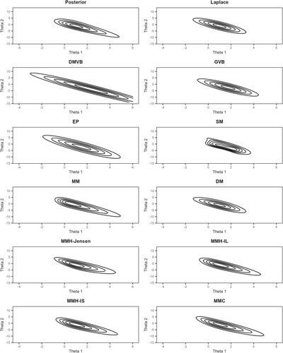
In general, the variants of the skew-normal matching method are seen to provide an increase in posterior fit compared to Gaussian approaches when p is not too high, at the cost of decreased speed. Better overall performance for the MM and MMC schemes may be achieved by only using them when an exact solution exists, and deferring to a Gaussian approximation otherwise. Figure 1 illustrates the benefits of the skew-normal matching method in a particular low-dimensional case with p = 2 and n = 4. Note that, for this specific example, approximate solutions were not needed for the MM and MMC schemes.

Figure 1. Contour plots for the posterior and across various approximation methods, for a small probit regression example with p = 2 and n = 4.

Results for the benchmark datasets are presented in Table 2. A similar hierarchy of performance to the simulations was observed among the skew-normal matching variants, with MM, MMC, and MMH generally performing better, and DM performing worse. Here, the SM approximation had higher $L^1$ accuracies compared to DM, but lower accuracies compared to the other skew-normal matching variants. The skew-normal matching method performed as well or better compared to its Gaussian approximation methods when p was not too high, as was the case for the German credit and Ionosphere datasets. For Ionosphere in particular, approximate solutions were required for the MM and MMC schemes. As with before, the skew-normal matching method comes with the cost of decreased speed. Similar points of discussion compared to the simulations can be made for the relative performance of the SM approximation across the benchmarks.

Table 2. Mean marginal $L^1$ accuracies (Acc.) (expressed as a percentage) across probit regression benchmarks. The highest accuracies for each benchmark dataset appear in bold.

	O-rings		Liver		Diabetes		Glass		Breast		Heart		German		Ion.
Method	Acc.	Time	Acc.	Time	Acc.	Time	Acc.	Time	Acc.	Time	Acc.	Time	Acc.	Time	Acc.	Time
Laplace	92.5	0.17	98.0	0.00	98.3	0.00	92.4	0.00	95.3	0.05	95.7	0.00	97.9	0.11	86.0	0.03
DMVB	95.5	0.14	99.1	0.19	99.2	0.61	96.9	0.33	97.1	1.97	99.1	0.74	99.2	31.00	93.2	10.85
GVB	96.5	0.33	99.1	0.09	99.2	0.06	97.3	2.16	98.2	2.12	99.0	0.09	99.2	0.46	97.3	11.54
EP	96.6	0.32	99.1	0.14	99.2	0.14	97.8	0.08	98.4	0.30	99.1	0.11	99.2	0.67	98.6	0.35
SM	96.9	0.91	99.2	1.14	99.0	1.62	96.2	2.03	97.9	1.81	98.5	2.61	99.0	4.47	90.5	6.05
MM	99.1	2.41	99.1	3.39	99.1	4.03	98.2	3.23	98.6	5.36	98.9	3.64	99.0	7.64	96.5	5.95
DM	95.7	0.31	98.3	0.11	98.4	0.12	52.9	0.14	96.2	0.17	97.1	0.21	95.3	0.42	86.4	0.46
MMH-Jensen	98.5	0.36	99.3	0.37	99.2	0.93	97.3	0.42	98.4	2.20	99.1	1.06	99.1	21.46	96.0	5.75
MMH-IL	98.6	0.53	99.3	2.19	99.2	6.01	97.5	3.64	98.4	21.26	99.0	4.90	99.1	125.89	97.1	39.86
MMH-IS	98.5	2.45	99.2	3.45	99.2	4.06	97.6	3.31	98.4	5.42	98.9	3.70	99.0	7.69	96.7	6.04
MMC	98.8	2.61	99.2	3.40	99.2	4.02	98.1	3.23	98.6	5.35	98.9	3.63	99.0	7.65	96.6	5.95

4.2. Post-hoc skewness adjustments

Simulation results for probit regression with independent covariates are shown in Tables 3 and 4. We have included the probit case because it showed the most promising results. The other cases are included in the supplementary material.

Table 3. Mean total marginal $L^1$ improvement/deterioration of accuracies (expressed as a percentage) across probit regression post-hoc simulations with independent covariate data. The column ‘+’ indicates a mean total improvement in marginal $L^1$ accuracy, while the column ‘−’ indicates the mean total decrease in marginal $L^1$ accuracy across simulations. For example, if the marginal improvements in $L^1$ accuracy for a p = 4 example were $(5,-2,1,-3)$, then the total marginal $L^1$ improvement and deterioration are 6 and 5 respectively. Pairs where there is an overall improvement are highlighted in bold. Long dashes indicate no data.

	p = 2		p = 4		p = 8		p = 16		p = 24		p = 40
Adjust.	+	−	+	−	+	−	+	−	+	−	+	−
$\mathbf{n}\mathbf{=}\mathbf{2}\mathbf{p}$
DMVB
MMH	22.1	1.5	57.7	1.2	153.4	0.9	271.3	3.7	395.9	5.9	644.1	16.1
MMC	3.2	0.4	5.4	0.1	4.5	0.0	7.0	0.0	4.9	0.0	–	–
GVB
MMH	16.6	0.7	33.4	3.1	48.6	7.3	76.3	14.6	74.6	26.4	104.4	66.1
MMC	3.8	0.1	3.2	0.3	2.8	0.2	1.5	0.2	–	–	–	–
EP
MMH	7.8	0.5	12.5	5.6	21.7	17.4	27.1	40.4	15.6	82.1	11.5	209.6
MMC	4.2	0.4	7.0	0.3	8.4	0.0	7.2	0.0	–	–	–	–
$\mathbf{n}\mathbf{=}\mathbf{4}\mathbf{p}$
DMVB
MMH	25.9	0.5	31.2	0.3	30.1	1.5	14.1	7.0	7.1	13.2	4.2	26.3
MMC	4.7	0.2	7.3	0.0	8.0	0.0	7.0	0.0	6.1	0.0	4.3	0.0
GVB
MMH	20.2	0.1	19.6	1.4	14.6	2.7	5.6	9.6	3.8	15.6	2.5	27.9
MMC	3.6	0.2	4.2	0.0	3.8	0.2	2.8	0.2	2.1	0.3	1.1	0.3
EP
MMH	11.7	0.2	12.3	2.1	9.2	4.0	3.7	13.4	2.4	20.6	1.2	35.5
MMC	2.7	1.1	5.4	0.4	5.7	0.1	4.6	0.1	3.6	0.1	2.0	0.1

Table 4. Success rates, i.e. rates where a solution exists to Algorithm 4, (expressed as a percentage) averaged over base approximations for the mean-mode-covariance based skewness adjustment. The mean-mode-Hessian based adjustments had a 100% success rate.

Multiplier	p = 2	p = 4	p = 8	p = 16	p = 24	p = 40
2	92.0	79.3	48.7	17.3	0.7	0.0
4	93.3	94.0	93.3	97.3	96.7	96.7

In the low data case, an MMH adjustment provided a noticeable increase in the quality of the posterior fit for the DMVB and GVB approximations, while a decrease in the quality of fit was seen for EP. On the other hand, MMC adjustments tended to increase or maintain $L^1$ accuracy for low values of p, with diminishing returns as p increased and exact solutions became rarer (as indicated by Table 4). In the moderate data case, the MMH adjustment was seen to increase $L^1$ accuracies across all methods for low values of p, but slightly decreased these accuracies for GVB and EP as p approached 40. In contrast, the MMC adjustment always increased or maintained the quality of the posterior fit. In general, simulations show that in most cases, some form of post-hoc skewness adjustment works reasonably well if the number of dimensions is not too high. The MMH adjustment gave very favourable results when there was low data (excluding EP, where it appeared to break down), while the MMC adjustment gave favourable results in all situations.

Results for the benchmarks are shown in Table 5. In the majority of cases, a post-hoc skewness adjustment was seen to give a slight improvement to the $L^1$ accuracy of the original Gaussian approximation. As with the simulations, MMH adjustments gave larger increases in $L^1$ accuracy but also had the risk of decreasing accuracy when p was large. This was seen with the Heart, German credit, and Ionosphere datasets. On the other hand, MMC adjustments tended to give more modest increases in accuracy but had a much lower chance of decreasing posterior fit. The German credit dataset appears to be an anomaly in this regard, and requires further investigation. In general, the benchmarks show that it is beneficial to apply some form of post-hoc skewness adjustment to an existing Gaussian approximation when the number of dimensions is not too high. Some approximations are also seen to benefit from a skewness adjustment more than others.

5. Summary and future work

This paper has introduced the skew-normal matching method as an alternative to standard Gaussian-based approximations of the posterior distribution, providing a potentially more practical and accurate alternative to the SM approximation of [9]. Four matching schemes are suggested, namely moment matching, derivative matching, mean-mode-Hessian matching, and mean-mode-covariance matching. Each scheme was based on matching a combination of derivatives at the mode and moments of the posterior with that of the multivariate SN density. The performance of these matching schemes was evaluated on a Bayesian probit regression model, where it was seen that for both simulated and benchmark data, the skew-normal matching method tended to outperform standard Gaussian-based approximations in terms of accuracy for low and moderate dimensions, at the cost of run time. In addition, all matching schemes except DM tended to outperform the SM approximation in the settings investigated. Each matching scheme is seen to offer a trade-off between performance and speed:

• Moment matching generally outperforms standard Gaussian approximations if an exact solution exists (more so than mean-mode-Hessian matching) and the dimensionality is not too high, but is compromised by an increase in run time with the estimation of the covariance and third moments, requiring importance sampling.

• Derivative matching offers an improvement in accuracy to the regular Laplace approximation when there is low data and the posterior is very skewed, at very little additional run time cost.

• Mean-mode-Hessian matching provides as or better performance compared to most standard Gaussian approximations when the dimensionality is not too high, at the cost of increased run time.

• Mean-mode-covariance matching generally outperforms standard Gaussian approximations if an exact solution exists (more so than mean-mode-Hessian matching) and the dimensionality is not too high, at the cost of increased run time with the estimation of the covariance, requiring importance sampling. Exact solutions are more frequent compared to moment matching.

Table 5. Mean total marginal improvement/deterioration in $L^1$ accuracies (expressed as a percentage) across probit regression post-hoc benchmarks. The ‘+’ columns indicates the total increases in marginal $L^1$ accuracy, while the ‘−’ column indicates the total decrease in marginal $L^1$ accuracy. For example, if the marginal improvements in $L^1$ accuracy for a p = 4 example were $(5,-2,1,-3)$, then the total marginal $L^1$ improvement and deterioration are 6 and 5 respectively. Pairs where there is an overall improvement are highlighted in bold. Long dashes indicate no data.

	O-rings		Liver		Diabetes		Glass		Breast		Heart		German		Ion.
Adjust.	+	–	+	–	+	–	+	–	+	–	+	–	+	–	+	–
DMVB
MMH	7.4	0.4	1.1	0.0	0.6	0.2	6.8	0.5	11.4	0.2	1.1	1.6	1.0	2.8	89.2	3.4
MMC	7.1	0.0	1.2	0.0	0.5	0.0	0.4	0.6	0.9	0.0	1.6	0.0	0.8	1.8	–	–
GVB
MMH	6.3	0.4	1.3	0.0	0.7	0.2	4.6	2.0	1.9	0.3	1.2	0.8	1.0	3.4	24.1	14.1
MMC	3.4	0.0	1.1	0.0	0.4	0.0	0.5	0.0	0.9	0.0	1.0	0.0	0.8	1.8	–	–
EP
MMH	6.4	0.4	1.3	0.0	0.7	0.3	1.8	3.4	1.4	1.2	1.0	1.0	1.0	3.0	1.7	34.0
MMC	4.1	0.0	1.2	0.0	0.4	0.0	0.5	0.4	0.9	0.0	1.0	0.0	0.8	1.9	–	–

The MMH and MMC schemes additionally gave way to post-hoc skewness adjustments for standard Gaussian approximations. For the case of probit regression, these adjustments were shown to generally result in increased marginal accuracies compared to the base approximation:

• Mean-mode-Hessian adjustments tend to give larger increases in marginal accuracies, but also risks decreasing these marginal accuracies when the dimensionality of the data is too large. Better performance was seen when there was low data.

• Mean-mode-covariance adjustments tend to give more modest increases in marginal accuracies but generally did not decrease marginal accuracies.

Although the skew-normal matching method has its benefits when the posterior is known to be skewed, this is not without its drawbacks. Using a matching, rather than an optimal variational approach can impact performance for some problems. This may explain why performance breaks down when the number of dimensions is large. We are also heavily dependent on good estimates of the moments; without these, the skew-normal approximation can fail very easily. For high dimensional data where $p\gg n$, skew normal matching is still possible, provided that the appropriate inverses exist to quantities such as the Hessian, although further work needs to be done in verifying the quality of these approximations.

There is clearly a variety of ways the work here could be extended. Other families of skewed densities could be entertained, the matching methods could be used as warm starts for skew-normal variational approximations [25,26], and matching with other posterior statistics is possible.

We hope that the results presented in this paper act as a benchmark for the performance of matching-based skewed approximations to posterior distributions. We believe that the skew-normal matching method fulfils a certain niche in posterior approximations and would like to see similar, if not better, methodologies being developed as approximate Bayesian inference grows and the need for such approximations increase.

Disclosure statement

The authors confirm that there are no relevant financial or non-financial competing interests to report.

Additional information

Funding

The work of John T. Ormerod was supported by an Australian Research Council Discovery Project Grant (DP210100521).

References

- Graves A. Practical variational inference for neural networks. Adv Neural Inf Process Syst. 2011;24:1–9.
- Zhou X, Hu Y, Liang W, et al. Variational LSTM enhanced anomaly detection for industrial big data. IEEE Trans Ind Inform. 2020;17(5):3469–3477. doi: 10.1109/TII.9424
- Tierney L, Kadane JB. Accurate approximations for posterior moments and marginal densities. J Am Stat Assoc. 1986;81(393):82–86. doi: 10.1080/01621459.1986.10478240
- Minka TP. A family of algorithms for approximate Bayesian inference [dissertation]. Massachusetts Institute of Technology; 2001.
- Blei DM, Kucukelbir A, McAuliffe JD. Variational inference: A review for statisticians. J Am Stat Assoc. 2017;112(518):859–877. doi: 10.1080/01621459.2017.1285773
- Gelman A, Carlin JB, Stern HS, et al. Bayesian data analysis. New York: Chapman and Hall/CRC; 1995.
- Fong Y, Rue H, Wakefield J. Bayesian inference for generalized linear mixed models. Biostatistics. 2010;11(3):397–412. doi: 10.1093/biostatistics/kxp053
- van Niekerk J, Rue H. Correcting the Laplace method with variational Bayes; 2021. arXiv preprint arXiv:211112945.
- Durante D, Pozza F, Szabo B. Skewed Bernstein-von Mises theorem and skew-modal approximations; 2023. ArXiv preprint arXiv:2301.03038.
- Genton MG, Loperfido NMR. Generalized skew-elliptical distributions and their quadratic forms. Ann Inst Stat Math. 2005;57(2):389–401. doi: 10.1007/BF02507031
- Wang J, Boyer J, Genton MG. A skew-symmetric representation of multivariate distributions. Stat Sin. 2004;14(4):1259–1270.
- Azzalini A. The multivariate skew-normal distribution. Biometrika. 1996;83(4):715–726. doi: 10.1093/biomet/83.4.715
- Azzalini A, Capitanio A. The skew-normal and related families. New York: Cambridge University Press; 2014.
- Chang CH, Lin JJ, Pal N, et al. A note on improved approximation of the binomial distribution by the skew-normal distribution. Am Stat. 2008;62(2):167–170. doi: 10.1198/000313008X305359
- Guolo A. A flexible approach to measurement error correction in case–control studies. Biometrics. 2008;64(4):1207–1214. doi: 10.1111/biom.2008.64.issue-4
- Gupta AK, Kollo T. Density expansions based on the multivariate skew normal distribution. Sankhyā: Indian J Stat. 2003;65(4):821–835.
- Vehtari A, Simpson D, Gelman A, et al. Pareto smoothed importance sampling; 2021. ArXiv preprint arXiv:1507.02646.
- R Core Team. R: A language and environment for statistical computing. Vienna, Austria: R Foundation for Statistical Computing; 2021.
- Stan Development Team. RStan: the R interface to Stan; 2023. R package version 2.21.8.
- Raudenbush SW, Yang ML, Yosef M. Maximum likelihood for generalized linear models with nested random effects via high-order, multivariate Laplace approximation. J Comput Graph Stat. 2000;9(1):141–157.
- Rue H, Martino S, Chopin N. Approximate Bayesian inference for latent Gaussian models by using integrated nested Laplace approximations. J R Stat Soc Series B Stat Methodol. 2009;71(2):319–392. doi: 10.1111/j.1467-9868.2008.00700.x
- Braun M, McAuliffe J. Variational inference for large-scale models of discrete choice. J Am Stat Assoc. 2010;105(489):324–335. doi: 10.1198/jasa.2009.tm08030
- Wang C, Blei DM. Variational inference in nonconjugate models. J Mach Learn Res. 2013;14(1):1005–1031.
- Mansournia MA, Geroldinger A, Greenland S, et al. Separation in logistic regression: causes, consequences, and control. Am J Epidemiol. 2018;187(4):864–870. doi: 10.1093/aje/kwx299
- Ormerod JT. Skew-normal variational approximations for Bayesian inference. Technical report. 2011.
- Smith MS, Loaiza-Maya R, Nott DJ. High-dimensional copula variational approximation through transformation. J Comput Graph Stat. 2020;29(4):729–743. doi: 10.1080/10618600.2020.1740097