Regularized estimation of Kronecker structured covariance matrix using modified Cholesky decomposition

Abstract

In this paper, we study a Kronecker structured model for covariance matrices when data are matrix-valued. Using the modified Cholesky decomposition for Kronecker structured covariance matrix, we propose a regularized covariance estimator by imposing shrinkage and smoothing penalties on the Cholesky factors. A regularized flip-flop (RFF) algorithm is developed to produce a statistically efficient estimator for a large covariance matrix of matrix-valued data. Asymptotic properties are investigated and the performance of the estimator is evaluated by simulations. The results presented are applied to real data example.

Keywords:

• Covariance matrix estimation
• Kronecker structure
• multivariate longitudinal data
• modified Cholesky decomposition
• regularization

1. Introduction

Matrix-valued data are commonly encountered in many practical problems such as environmental science [1], image analysis [2] and electrical engineering [3], to mention a few, when the observations are collected from two different dimensions such as spatial-temporal data with measurements at different locations observed repeatedly over a few times. Kronecker product covariance matrix, which can be represented as a Kronecker product of two covariance matrices, plays an important role when separability of the covariance structure is assumed for the matrix-valued data. The term ‘separability’ comes from the assumption that the temporal correlation is the same for all locations and similarly the spatial correlation is the same for all time points (Kronecker product covariance matrix is also called separable covariance matrix). That is saying, for the spatial-temporal data, the covariance matrix can be represented as a Kronecker product of a covariance matrix $\mathbf{\Sigma }$ which modelling the dependence over the locations and another covariance matrix $\mathbf{\Psi }$ which modelling the dependence over the time points.

Using a Kronecker product covariance matrix whenever possible is advantageous since compared with the totally unstructured covariance matrix, it consists of less number of unknown parameters, and at the same time, the separability property for a covariance structure captures the important dependence present in the data. More recently, Bucci et al. [4] proposed a method of forecasting covariance matrices through a parametrization of the matrices. Yang and Kang [5] introduced a way for matrix decomposition for the large banded covariance matrix. Jurek and Katzfuss [6] investigated an algorithm as a hierarchical Vecchia approximation to estimate both covariance matrix and the precision matrix. It should be mentioned, that in some circumstances, it will be reasonable to assume further structures on both $\mathbf{\Sigma }$ and $\mathbf{\Psi }$, which further reduces the number of unknown parameters, see Filipiak and Klein [7], Hao et al. [8], Szczepańska-Álvarez et al. [9] for instance. However, the statistical inference of Kronecker product covariance matrix has faced some challenges, especially regarding the estimating procedure. Among others, this type of structure has a non-identifiability issue which means the estimators will not be unique without imposing a restriction on the parameters. Srivastava et al. [10] imposed a restriction on the matrix $\mathbf{\Psi }$, i.e. ${\psi }_{11}=1$ and proved the uniqueness of maximum likelihood estimators (MLEs) of $\mathbf{\Sigma }$ and $\mathbf{\Psi }$ via the flip-flop algorithm.

Nowadays datasets are becoming increasingly large and may be high-dimensional, that is, the number of variables is bigger than the sample size. In a high-dimensional situation, obtaining a stable and efficient estimator for the covariance matrix is difficult, which is one major obstacle in modelling covariance matrices. It has been already pointed out in the 1950s by Stein [11] that the MLE of the covariance matrix, the sample covariance matrix, is not a good estimator when the matrix dimension is relatively or very large with respect to the sample size. The other major obstacle is to preserve positive definiteness of covariance matrices. Many good methods have been developed during the years under the assumption of sparsity of the high-dimensional covariance matrix, for example, the generalized thresholding method [12] and the blocked thresholding method [13]. However, these regularized methods do not guarantee the covariance estimator is positive definite.

To overcome these obstacles, the study of high-dimensional covariance estimation has paid a lot of attention to the framework of the modified Cholesky decomposition (MCD). MCD is a completely unconstrained and interpretable reparameterization of a covariance matrix [14,15]. Bickel and Levina [16] showed that banding the Cholesky factor can produce a consistent estimator in the operator norm under weak assumptions on the covariance matrix. Huang et al. [17] showed that shrinkage is very useful in providing a more stable estimate of a covariance matrix, especially when the dimension is high. Dai et al. [18] proposed a new type of Mahalanobis distance based on the regularized estimator of precision matrix.

Imposing only regularization on MCD ignores the dependence among the neighbouring elements of the covariance matrix which is a natural property for longitudinal data. In this paper, we adopt the idea of Tai [19] and employ not only shrinkage but also smoothing penalty. The proposed regularization scheme of Dai et al. [18] was motivated by two observations of the Cholesky factor. Firstly, the Cholesky factor is likely to have many off-diagonal elements that are zero or close to zero. Secondly, continuity is a natural property among neighbouring elements of the Cholesky factor for the covariance matrices of longitudinal data. Taking smoothness into account can help to provide more efficient covariance matrix estimates.

This paper aims to obtain regularized MLEs for ${\mathbf{\Sigma }}_{p\times p}$ and ${\mathbf{\Psi }}_{q\times q}$ which are computationally feasible when p, q are large, as well as to develop exploratory tools to investigate further structures of column/row covariance matrices of the matrix-valued data. The novelty of this paper is that the separability assumption is taken into account and the regularization techniques are incorporated when estimating the covariance of matrix-valued data using MCD. A so-called regularized flip-flop algorithm (RFF) will be proposed in a later section.

The rest of the paper is organized as follows. In Section 2, we introduce the modified Cholesky decomposition and the extension when it is applied to the Kronecker product covariance structures as well as review the MLE procedure of this type of covariance structure. In Section 3, we propose regularized estimators of $\mathbf{\Sigma }$ and $\mathbf{\Psi }$ based on combining shrinkage and smoothing. The main theoretical results are presented in Section 4. A simulation study is conducted in Section 5 to evaluate the performance of the proposed estimators. In Section 6 the obtained results are illustrated with a real data example. Some discussions are given in Section 7.

Throughout the paper, we use the following notations. For a matrix $\mathbf{A}$, ${\mathbf{A}}^{\prime }$ denotes the transpose, $\mathrm{tr}(\mathbf{A})$ is the trace, ${\mathbf{A}}^{-1}$ is the inverse matrix, $\det (\mathbf{A})$ is the determinant, $\mathrm{diag}(\mathbf{A})$ is the diagonalizing operator and $\mathrm{vec}(\mathbf{A})$ is the vectorizing operator of $\mathbf{A}$, respectively. Moreover, $\Vert \mathbf{A}{\Vert }_F^2=\mathrm{tr}({\mathbf{A}}^{\prime }\mathbf{A})$, $\Vert \mathbf{A}\Vert ={\lambda }_{max}^{1/2}({\mathbf{A}}^{\prime }\mathbf{A})$ and the matrix $\mathbf{A}\otimes \mathbf{B}$ denotes the Kronecker product of $\mathbf{A}$ and $\mathbf{B}$. As such, ${\mathbf{A}}^{\otimes 2}$ denotes the Kronecker product of $\mathbf{A}$ and $\mathbf{A}$. ${\mathbf{A}}_0$ denotes the true parameter of the underlying model. Operators $O(\bullet )$ and $o(\bullet )$ are the infinitely large quantity and infinitely small quantity, and $O_P(\bullet )$ and $o_P(\bullet )$ denote that relationships hold with probability tending to 1.

2. Modified Cholesky decomposition of a Kronecker product covariance structure

In this section, we will first give a short review of MCD. Then we present the MLE of the Kronecker product covariance structure. The MLE is provided by using an iterative algorithm which is referred to as the ‘flip-flop algorithm’ [20]. At the end of this section, the MCD of the Kronecker product covariance structure is given.

2.1. Modified Cholesky decomposition

Suppose that $\mathit{Y}$ is a random matrix which consists of n independent p-dimensional random vectors with mean $\mathbf{0}$ and the covariance matrix $\mathbf{\Lambda }$. Let $\mathit{Y}$ follow $N_{p,n}(\mathbf{0},\mathbf{\Lambda },{\mathbf{I}}_n)$. With a covariance matrix $\mathbf{\Lambda }$ of order p, the modified Cholesky decomposition [14] of $\mathbf{\Lambda }$ is specified by (1) $\mathbf{T}\mathbf{\Lambda }{\mathbf{T}}^{\prime }=\mathbf{D},$(1) and thus, $\mathbf{\Lambda }={\mathbf{T}}^{-1}\mathbf{D}{\mathbf{T}}^{\prime -1}$, where $\mathbf{T}$ is a unique unit lower triangular matrix with ones on the main diagonal and $\mathbf{D}$ is a unique diagonal matrix, i.e. $\begin{array}{r}\mathbf{T}=\left(\begin{array}{ccccc}1& 0& 0& \cdots & 0\\ -{\varphi }_{21}& 1& 0& \cdots & 0\\ -{\varphi }_{31}& -{\varphi }_{32}& 1& \cdots & 0\\ ⋮& ⋮& \ddots & \ddots & ⋮\\ -{\varphi }_{p1}& -{\varphi }_{p2}& \cdots & -{\varphi }_{p(p-1)}& 1\end{array}\right)\mathrm{and}\mathbf{D}=\left(\begin{array}{cccc}{\sigma }_1^2& 0& \cdots & 0\\ 0& {\sigma }_2^2& \cdots & 0\\ ⋮& ⋮& \ddots & ⋮\\ 0& 0& \cdots & {\sigma }_p^2\end{array}\right).\end{array}$Based on Equation (1(1) $\mathbf{T}\mathbf{\Lambda }{\mathbf{T}}^{\prime }=\mathbf{D},$(1) ) and the property that normality is preserved under linear transformations, we have (2) $\mathbf{T}\mathit{Y}=\mathbf{E},\mathbf{E}\sim N(\mathbf{0},\mathbf{D},{\mathbf{I}}_n),$(2) which turns out that Equation (2(2) $\mathbf{T}\mathit{Y}=\mathbf{E},\mathbf{E}\sim N(\mathbf{0},\mathbf{D},{\mathbf{I}}_n),$(2) ) can be represented as the following linear model: (3) ${\mathbf{y}}_t=\sum _{k=1}^{t-1}{\varphi }_{tk}{\mathbf{y}}_k+{\mathbf{e}}_t,{\mathbf{e}}_t\sim N(\mathbf{0},{\sigma }_k^2{\mathbf{I}}_n),t=2,\dots ,p,$(3) where ${\varphi }_{tk}$ and ${\sigma }_k^2$ are the generalized autoregressive parameters and innovation variances, respectively. Observing Equation (2(2) $\mathbf{T}\mathit{Y}=\mathbf{E},\mathbf{E}\sim N(\mathbf{0},\mathbf{D},{\mathbf{I}}_n),$(2) ) has been split into p independent simple linear regression models and the MLEs of the unknown parameters in (3(3) ${\mathbf{y}}_t=\sum _{k=1}^{t-1}{\varphi }_{tk}{\mathbf{y}}_k+{\mathbf{e}}_t,{\mathbf{e}}_t\sim N(\mathbf{0},{\sigma }_k^2{\mathbf{I}}_n),t=2,\dots ,p,$(3) ) are actually ordinary least squares (OLS) estimators. It can be seen that MCD provides an alternative MLE estimation procedure of $\mathbf{\Lambda }$ through a sequential regression scheme, which reduces the challenge of estimating a covariance matrix.

2.2. Maximum likelihood estimation

Let ${\mathbf{X}}_i$ be a random matrix which is normally distributed and we can write (4) ${\mathbf{X}}_i\sim N_{p,q}(\mathit{\mu },\mathbf{\Sigma },\mathbf{\Psi }),i=1,\dots ,n,$(4) where $\mathit{\mu }$ is an $p\times q$ unstructured mean, $\mathbf{\Sigma }$ is an $p\times p$ unstructured covariance between rows of ${\mathbf{X}}_i$ at any given column and $\mathbf{\Psi }$ is an $q\times q$ unstructured covariance between columns of ${\mathbf{X}}_i$ at any given row. Both $\mathbf{\Sigma }$ and $\mathbf{\Psi }$ are unknown, positive definite matrices. Without loss of generality, we consider the case $\mathit{\mu }=\mathbf{0}$. Equivalently, the vectorized version of model (4(4) ${\mathbf{X}}_i\sim N_{p,q}(\mathit{\mu },\mathbf{\Sigma },\mathbf{\Psi }),i=1,\dots ,n,$(4) ) can be written as (5) $\mathrm{vec}{\mathbf{X}}_i\sim N_{pq}(\mathbf{0},\mathbf{\Psi }\otimes \mathbf{\Sigma }).$(5) How to estimate the covariance structure $\mathbf{\Psi }\otimes \mathbf{\Sigma }$ in Equation (5(5) $\mathrm{vec}{\mathbf{X}}_i\sim N_{pq}(\mathbf{0},\mathbf{\Psi }\otimes \mathbf{\Sigma }).$(5) ) has been discussed intensively in the statistical literature, especially in the MLE framework, see, e.g. Galecki [21], Lu and Zimmerman [20], Manceur and Dutilleul [22], Naik and Rao [23], Roy and Khattree [24]. The log-likelihood function of (5(5) $\mathrm{vec}{\mathbf{X}}_i\sim N_{pq}(\mathbf{0},\mathbf{\Psi }\otimes \mathbf{\Sigma }).$(5) ) is (6) $-2\ln L=c+n\ln [det(\mathbf{\Psi }\otimes \mathbf{\Sigma })]+\sum _{i=1}^n\left[ve{c}^{\prime }{\mathbf{X}}_i({\mathbf{\Psi }}^{-1}\otimes {\mathbf{\Sigma }}^{-1})vec{\mathbf{X}}_i\right],$(6) where $c=npq\ln (2\pi )$. It has been noticed that there is no explicit expression for the MLE of both $\mathbf{\Sigma }$ and $\mathbf{\Psi }$, and the reason is that there are no analytical solutions to the system of two matrix equations below: (7) $np\hat{\mathbf{\Sigma }}=\sum _{i=1}^n{\mathbf{X}}_{ic}{\hat{\mathbf{\Psi }}}^{-1}{\mathbf{X}}_{ic}^{\prime },nq\hat{\mathbf{\Psi }}=\sum _{i=1}^n{\mathbf{X}}_{ic}{\hat{\mathbf{\Sigma }}}^{-1}{\mathbf{X}}_{ic}^{\prime },$(7) where ${\mathbf{X}}_{ic}={\mathbf{X}}_i-\hat{\mathit{\mu }}$ and $\hat{\mathit{\mu }}$ is $\frac{1}{n}\sum _{i=1}^n{\mathbf{X}}_i$, $i=1,2,\dots ,n$. An iterative algorithm, the flip-flop algorithm, is therefore required and it proceeds by iteratively updating $\mathbf{\Sigma }$ and $\mathbf{\Psi }$, and iterations continue until some convergence criterion is fulfilled, e.g. the Euclidean distance between successive Kronecker product estimates is smaller than some given threshold. Regarding conditions on the sample size n for the existence of the MLE of a Kronecker product covariance matrix, see Table 1 of Dutilleul [25] for a summary. Nevertheless, for positive definiteness of the estimators $\mathbf{\Sigma }$ and $\mathbf{\Psi }$, the sample size n must be greater than p and greater than q, giving $n>\max (p,q)$, which was suggested by Srivastava et al. [10].

It is worth mentioning that there is an unidentifiable issue in $\mathbf{\Psi }\otimes \mathbf{\Sigma }$ since $(c\mathbf{\Psi })\otimes (c^{-1}\mathbf{\Sigma })=\mathbf{\Psi }\otimes \mathbf{\Sigma }$ for any constant c, see, e.g. Galecki [21], Naik and Rao [23]. Thus, for the purpose of identifiability, we shall assume the first element of $\mathbf{\Psi }$ as ${\psi }_{11}=1$. Denote ${\mathbf{\Psi }}^{\ast }$ as $\mathbf{\Psi }$ under the restriction ${\psi }_{11}=1$.

2.3. MCD of a Kronecker product covariance structure

The estimating equations in (7(7) $np\hat{\mathbf{\Sigma }}=\sum _{i=1}^n{\mathbf{X}}_{ic}{\hat{\mathbf{\Psi }}}^{-1}{\mathbf{X}}_{ic}^{\prime },nq\hat{\mathbf{\Psi }}=\sum _{i=1}^n{\mathbf{X}}_{ic}{\hat{\mathbf{\Sigma }}}^{-1}{\mathbf{X}}_{ic}^{\prime },$(7) ) will look different depending on the structures of $\mathbf{\Sigma }$ and $\mathbf{\Psi }$. Szczepańska-Álvarez et al. [9] studied four Kronecker product covariance structures by imposing different restrictions on the pair of matrices $\mathbf{\Sigma }$, $\mathbf{\Psi }$. The authors have obtained likelihood estimation equations for these covariance structures which give the possibility to utilize flip-flop type algorithms with clear stopping rules.

In this subsection, we consider MCD of the covariance matrix $\mathbf{\Lambda }={\mathbf{\Psi }}^{\ast }\otimes \mathbf{\Sigma }$. The following theorem provides us with an important result concerning the parameter space of ${\mathbf{\Psi }}^{\ast }\otimes \mathbf{\Sigma }$ when the MCD is performed.

Theorem 2.1

Let $\mathbf{\Lambda }={\mathbf{\Psi }}^{\ast }\otimes \mathbf{\Sigma }$, the unique MCD for $\mathbf{\Lambda }$ such that $\mathbf{T}\mathbf{\Lambda }{\mathbf{T}}^{\prime }=\mathbf{D}$ has the following pattern: $\mathbf{T}={\mathbf{T}}_2\otimes {\mathbf{T}}_1,\mathbf{D}={\mathbf{D}}_2^{\ast }\otimes {\mathbf{D}}_1,$where ${\mathbf{T}}_1=(-{\varphi }_{tj}):p\times p$ and ${\mathbf{T}}_2=(-{\eta }_{sk}):q\times q$ are two different unique unit lower triangular matrices, $1\le t\le p$, $1\le j\le t-1$, $1\le s\le q$, $1\le k\le s-1$. The matrices ${\mathbf{D}}_1=\mathrm{diag}({\sigma }_1^2,\dots ,{\sigma }_p^2)$ and ${\mathbf{D}}_2^{\ast }=\mathrm{diag}(1,{\gamma }_2^2,\dots ,{\gamma }_q^2)$ are two different diagonal matrices.

Proof.

Since $\mathbf{T}$ is a unique unit lower triangular matrix, it can be reformulated as $\mathbf{T}={\mathbf{T}}_2\otimes {\mathbf{T}}_1$, where ${\mathbf{T}}_1$ and ${\mathbf{T}}_2$ are also triangular matrices. Then we have $\mathbf{T}\mathbf{\Lambda }{\mathbf{T}}^{\prime }=({\mathbf{T}}_2\otimes {\mathbf{T}}_1)({\mathbf{\Psi }}^{\ast }\otimes \mathbf{\Sigma })({\mathbf{T}}_2\otimes {\mathbf{T}}_1{)}^{\prime }={\mathbf{T}}_2{\mathbf{\Psi }}^{\ast }{\mathbf{T}}_2^{\prime }\otimes {\mathbf{T}}_1\mathbf{\Sigma }{\mathbf{T}}_1^{\prime }={\mathbf{D}}_2^{\ast }\otimes {\mathbf{D}}_1.$Observing that under the identifiable restriction ${\psi }_{11}=1$, it follows that ${\mathbf{D}}_2^{\ast }={\mathbf{T}}_2{\mathbf{\Psi }}^{\ast }{\mathbf{T}}_2^{\prime }$, which implies that ${\gamma }_1^2=1$. On the other hand, if ${\gamma }_1^2=1$, based on the fact ${\mathbf{\Psi }}^{\ast }={\mathbf{T}}_2^{-1}{\mathbf{D}}_2^{\ast }({\mathbf{T}}_2^{-1}{)}^{\prime }$, where ${\mathbf{T}}_2^{-1}$ is also a unit triangular matrix [26], hence we have ${\psi }_{11}=1$ in $\mathbf{\Psi }$, i.e. ${\mathbf{\Psi }}^{\ast }$.

The results in Theorem 2.1 reveal that the MCD of Kronecker product covariance structure also has a Kronecker product pattern and it is a one-to-one transformation of the original parameter space. Moreover, the identifiable restriction ${\psi }_{11}=1$ only affects the diagonal matrix ${\mathbf{D}}_2^{\ast }$ and does not affect the matrices ${\mathbf{T}}_1$ and ${\mathbf{T}}_2$, which is important when we introduce the penalty terms in the next section.

3. Regularized estimation of Kronecker product covariance structure

Using Theorem 2.1 and the property that matrix-variate normality is preserved under linear transformations, model (4(4) ${\mathbf{X}}_i\sim N_{p,q}(\mathit{\mu },\mathbf{\Sigma },\mathbf{\Psi }),i=1,\dots ,n,$(4) ) gives ${\mathbf{T}}_1{\mathbf{X}}_i{\mathbf{T}}_2^{\prime }\sim N_{p,q}(\mathbf{0},{\mathbf{D}}_1,{\mathbf{D}}_2^{\ast })$. With the facts $\mathbf{\Sigma }={\mathbf{T}}_1^{-1}{\mathbf{D}}_1({\mathbf{T}}_1^{-1}{)}^{\prime }$, ${\mathbf{\Psi }}^{\ast }={\mathbf{T}}_2^{-1}{\mathbf{D}}_2^{\ast }({\mathbf{T}}_2^{-1}{)}^{\prime }$, ${{\mathbf{\Psi }}^{\ast }}^{-1}\otimes {\mathbf{\Sigma }}^{-1}=({\mathbf{T}}_2^{\prime }\otimes {\mathbf{T}}_1^{\prime })({{\mathbf{D}}_2^{\ast }}^{-1}\otimes {\mathbf{D}}_1^{-1})({\mathbf{T}}_2\otimes {\mathbf{T}}_1)$ and $({\mathbf{T}}_2\otimes {\mathbf{T}}_1)\mathrm{vec}{\mathbf{X}}_i=\mathrm{vec}({\mathbf{T}}_1{\mathbf{X}}_i{\mathbf{T}}_2^{\prime })$, the log-likelihood function given in (6(6) $-2\ln L=c+n\ln [det(\mathbf{\Psi }\otimes \mathbf{\Sigma })]+\sum _{i=1}^n\left[ve{c}^{\prime }{\mathbf{X}}_i({\mathbf{\Psi }}^{-1}\otimes {\mathbf{\Sigma }}^{-1})vec{\mathbf{X}}_i\right],$(6) ), can be expressed as (8) $\begin{array}{rl}& \ln L({\mathbf{D}}_1,{\mathbf{T}}_1,{\mathbf{D}}_2,{\mathbf{T}}_2)=c+n\ln [det({\mathbf{T}}_2^{-1}\otimes {\mathbf{T}}_1^{-1})]+n\ln [det({\mathbf{D}}_2^{\ast }\otimes {\mathbf{D}}_1)]\\ & +\sum _{i=1}^n\left[{\mathrm{vec}}^{\prime }{\mathbf{X}}_i{({\mathbf{T}}_2\otimes {\mathbf{T}}_1)}^{\prime }({{\mathbf{D}}_2^{\ast }}^{-1}\otimes {\mathbf{D}}_1^{-1})({\mathbf{T}}_2\otimes {\mathbf{T}}_1)\mathrm{vec}{\mathbf{X}}_i\right]\\ & =c+n\ln [det({\mathbf{D}}_2^{\ast }\otimes {\mathbf{D}}_1)]+\sum _{i=1}^n\mathrm{tr}({\mathbf{X}}_i^{\prime }{\mathbf{T}}_1^{\prime }{\mathbf{D}}_1^{-1}{\mathbf{T}}_1{\mathbf{X}}_i{\mathbf{T}}_2^{\prime }{{\mathbf{D}}_2^{\ast }}^{-1}{\mathbf{T}}_2)\\ & =c+np\sum _{s=1}^q\ln {\gamma }_s^{-2}+nq\sum _{t=1}^p\ln {\sigma }_t^{-2}+\sum _{i=1}^n\mathrm{tr}[({\mathbf{T}}_1{\mathbf{X}}_i{\mathbf{T}}_2^{\prime }){{\mathbf{D}}_2^{\ast }}^{-1}({\mathbf{T}}_1{\mathbf{X}}_i{\mathbf{T}}_2^{\prime }{)}^{\prime }{\mathbf{D}}_1^{-1}].\end{array}$(8) We will now discuss how to estimate $\mathbf{\Lambda }={\mathbf{\Psi }}^{\ast }\otimes \mathbf{\Sigma }$ when both $\mathbf{\Sigma }$ and ${\mathbf{\Psi }}^{\ast }$ have patterned structures (certain parsimonies) such as first-order autoregressive (AR(1)) and compound symmetry (CS). Parsimony in a covariance matrix leads to parsimony in the Cholesky factor, which corresponds to many zeros or small elemetns in the regression coefficients. For example, for an AR(1) covariance matrix, there could be considerable amount of zeros in the subdiagonals of the $\mathbf{T}$ matrices. In particular, the first subdiagonal of $\mathbf{T}$ has the same entry in all places, and the rest of the subdiagonals are either zero or contain minor values that are close to zero. For a CS covariance matrix, the elements of each row of the Cholesky factor matrix are the same, and one can expect that there are many small value elements in the last few rows of the lower triangular part of $\mathbf{T}$. One can observe that, with a specific pattern for $\mathbf{\Sigma }$ and ${\mathbf{\Psi }}^{\ast }$, the corresponding Cholesky factor matrix components in Theorem 2.1, ${\mathbf{T}}_m$ matrices where m = 1, 2, are potentially sparse or nearly sparse.

In order to take into account both sparsity and smoothness, we apply the $L_1$ penalty which shrinks the estimates of ${\varphi }_{tj}$'s and ${\eta }_{sk}$'s toward zero, and at the same time introduce the smoothing penalties in the framework of penalized likelihood. The shrinkage penalties are given as follows: (9) ${\lambda }_{sh,1}\sum _{t=2}^p\sum _{j=1}^{t-1}\left|{\varphi }_{tj}\right|,{\lambda }_{sh,2}\sum _{s=2}^q\sum _{k=1}^{s-1}\left|{\eta }_{sk}\right|,$(9) where ${\lambda }_{sh,1}$ and ${\lambda }_{sh,2}$ are the shrinkage tuning parameters. The smoothing penalties have the forms (10) ${\lambda }_{sm,1}\sum _{t=2}^{p-2}\sum _{j=1}^{t-1}({\mathrm{\Delta }}_{diag}^2{\varphi }_{t+2,t+2-j}{)}^2,{\lambda }_{sm,2}\sum _{s=2}^{q-2}\sum _{k=1}^{s-1}({\mathrm{\Delta }}_{diag}^2{\eta }_{s+2,s+2-k}{)}^2,$(10) where ${\lambda }_{sm,1}$ and ${\lambda }_{sm,2}$ are the smoothing tuning parameters, and $\begin{array}{rl}& {\mathrm{\Delta }}_{diag}^2{\varphi }_{t+2,t+2-j}=({\varphi }_{t+2,t+2-j}-{\varphi }_{t+1,t+1-j})-({\varphi }_{t+1,t+1-j}-{\varphi }_{t,t-j}),\\ & {\mathrm{\Delta }}_{diag}^2{\eta }_{s+2,s+2-k}=({\eta }_{s+2,s+2-k}-{\eta }_{s+1,s+1-k})-({\eta }_{s+1,s+1-k}-{\eta }_{s,s-k}),\end{array}$are the second order differences of ${\mathbf{T}}_1$ and ${\mathbf{T}}_2$, respectively. Combining the penalties given in (9(9) ${\lambda }_{sh,1}\sum _{t=2}^p\sum _{j=1}^{t-1}\left|{\varphi }_{tj}\right|,{\lambda }_{sh,2}\sum _{s=2}^q\sum _{k=1}^{s-1}\left|{\eta }_{sk}\right|,$(9) ) and (10(10) ${\lambda }_{sm,1}\sum _{t=2}^{p-2}\sum _{j=1}^{t-1}({\mathrm{\Delta }}_{diag}^2{\varphi }_{t+2,t+2-j}{)}^2,{\lambda }_{sm,2}\sum _{s=2}^{q-2}\sum _{k=1}^{s-1}({\mathrm{\Delta }}_{diag}^2{\eta }_{s+2,s+2-k}{)}^2,$(10) ), the penalized likelihood function can be presented as: (11) $\begin{array}{rl}& -2\log L+{\lambda }_{sh,1}\sum _{t=2}^p\sum _{j=1}^{t-1}\left|{\varphi }_{tj}\right|+{\lambda }_{sm,1}\sum _{t=2}^{p-2}\sum _{j=1}^{t-1}({\mathrm{\Delta }}_{diag}^2{\varphi }_{t+2,t+2-j}{)}^2\\ & +{\lambda }_{sh,2}\sum _{s=2}^q\sum _{k=1}^{s-1}\left|{\eta }_{sk}\right|+{\lambda }_{sm,2}\sum _{s=2}^{q-2}\sum _{k=1}^{s-1}({\mathrm{\Delta }}_{diag}^2{\eta }_{s+2,s+2-k}{)}^2,\end{array}$(11) where $-2\log L$ is given in (8(8) $\begin{array}{rl}& \ln L({\mathbf{D}}_1,{\mathbf{T}}_1,{\mathbf{D}}_2,{\mathbf{T}}_2)=c+n\ln [det({\mathbf{T}}_2^{-1}\otimes {\mathbf{T}}_1^{-1})]+n\ln [det({\mathbf{D}}_2^{\ast }\otimes {\mathbf{D}}_1)]\\ & +\sum _{i=1}^n\left[{\mathrm{vec}}^{\prime }{\mathbf{X}}_i{({\mathbf{T}}_2\otimes {\mathbf{T}}_1)}^{\prime }({{\mathbf{D}}_2^{\ast }}^{-1}\otimes {\mathbf{D}}_1^{-1})({\mathbf{T}}_2\otimes {\mathbf{T}}_1)\mathrm{vec}{\mathbf{X}}_i\right]\\ & =c+n\ln [det({\mathbf{D}}_2^{\ast }\otimes {\mathbf{D}}_1)]+\sum _{i=1}^n\mathrm{tr}({\mathbf{X}}_i^{\prime }{\mathbf{T}}_1^{\prime }{\mathbf{D}}_1^{-1}{\mathbf{T}}_1{\mathbf{X}}_i{\mathbf{T}}_2^{\prime }{{\mathbf{D}}_2^{\ast }}^{-1}{\mathbf{T}}_2)\\ & =c+np\sum _{s=1}^q\ln {\gamma }_s^{-2}+nq\sum _{t=1}^p\ln {\sigma }_t^{-2}+\sum _{i=1}^n\mathrm{tr}[({\mathbf{T}}_1{\mathbf{X}}_i{\mathbf{T}}_2^{\prime }){{\mathbf{D}}_2^{\ast }}^{-1}({\mathbf{T}}_1{\mathbf{X}}_i{\mathbf{T}}_2^{\prime }{)}^{\prime }{\mathbf{D}}_1^{-1}].\end{array}$(8) ).

The maximizer of (11(11) $\begin{array}{rl}& -2\log L+{\lambda }_{sh,1}\sum _{t=2}^p\sum _{j=1}^{t-1}\left|{\varphi }_{tj}\right|+{\lambda }_{sm,1}\sum _{t=2}^{p-2}\sum _{j=1}^{t-1}({\mathrm{\Delta }}_{diag}^2{\varphi }_{t+2,t+2-j}{)}^2\\ & +{\lambda }_{sh,2}\sum _{s=2}^q\sum _{k=1}^{s-1}\left|{\eta }_{sk}\right|+{\lambda }_{sm,2}\sum _{s=2}^{q-2}\sum _{k=1}^{s-1}({\mathrm{\Delta }}_{diag}^2{\eta }_{s+2,s+2-k}{)}^2,\end{array}$(11) ) does not have a closed-form expression. Hence, we extend the flip-flop algorithm [20,27] to incorporate the $L_1$ penalties in (9(9) ${\lambda }_{sh,1}\sum _{t=2}^p\sum _{j=1}^{t-1}\left|{\varphi }_{tj}\right|,{\lambda }_{sh,2}\sum _{s=2}^q\sum _{k=1}^{s-1}\left|{\eta }_{sk}\right|,$(9) ) and smoothing penalties in (10(10) ${\lambda }_{sm,1}\sum _{t=2}^{p-2}\sum _{j=1}^{t-1}({\mathrm{\Delta }}_{diag}^2{\varphi }_{t+2,t+2-j}{)}^2,{\lambda }_{sm,2}\sum _{s=2}^{q-2}\sum _{k=1}^{s-1}({\mathrm{\Delta }}_{diag}^2{\eta }_{s+2,s+2-k}{)}^2,$(10) ). We estimate the matrices ${\mathbf{T}}_1,{\mathbf{T}}_2,{\mathbf{D}}_1,{\mathbf{D}}_2^{\ast }$ based on the following steps.

Step 1: With fixed ${\mathbf{T}}_2$ and ${\mathbf{D}}_2^{\ast }$, update ${\mathbf{T}}_1$, ${\mathbf{D}}_1$ with $\begin{array}{rl}& \sum _{t=1}^p(nq\log {\sigma }_t^2+\Vert {\mathbf{u}}_t-\sum _{k=1}^{t-1}{\varphi }_{tk}{\mathbf{u}}_k{\Vert }^2{\sigma }_t^{-2})\\ & +{\lambda }_{sh,1}\sum _{t=2}^p\sum _{k=1}^{t-1}|{\varphi }_{tk}|+{\lambda }_{sm,1}\sum _{t=2}^{p-2}\sum _{k=1}^{t-1}({\mathrm{\Delta }}_{diag}^2{\varphi }_{t+2,t+2-k}{)}^2,\end{array}$Step 2: With fixed ${\mathbf{T}}_1$ and ${\mathbf{D}}_1$, update ${\mathbf{T}}_2$, ${\mathbf{D}}_2^{\ast }$, with $\begin{array}{rl}& \sum _{s=1}^q(np\log {\gamma }_s^2+\Vert {\mathbf{v}}_s-\sum _{k=1}^{s-1}{\eta }_{sk}{\mathbf{v}}_k{\Vert }^2{\gamma }_s^{-2})\\ & +{\lambda }_{sh,2}\sum _{s=2}^q\sum _{k=1}^{s-1}|{\eta }_{sk}|+{\lambda }_{sm,2}\sum _{s=2}^{q-2}\sum _{k=1}^{s-1}({\mathrm{\Delta }}_{diag}^2{\eta }_{s+2,s+2-k}{)}^2,\end{array}$where ${\mathbf{u}}_t^{\prime }$ is the tth row of the mode 1 unfolding of $\mathbf{U}=[{\mathbf{X}}_1^{\prime }:\cdots :{\mathbf{X}}_n^{\prime }{]}^{\prime }{\mathbf{T}}_2^{\prime }{\mathbf{D}}_2^{\ast -1/2}$ and ${\mathbf{v}}_s$ is the sth column of the mode 2 unfolding of $\mathbf{V}={\mathbf{D}}_{\mathbf{1}}^{\mathbf{-}\mathbf{1}\mathbf{/}\mathbf{2}}{\mathbf{T}}_{\mathbf{1}}\mathbf{[}{\mathbf{X}}_{\mathbf{1}}\mathbf{:}\cdots \mathbf{:}{\mathbf{X}}_{\mathbf{n}}\mathbf{]}$. The pseudo-code of the algorithm, the regularized flip-flop (RFF) algorithm, is described in Algorithm 1 in Appendix 3.

4. Main results: theoretical convergence

This section shows the asymptotic properties of the proposed estimator. We start with some assumptions that are needed for the theoretical analysis of the penalized likelihood function.

Let $s_1$ and $s_2$ be the number of nonzero elements in the lower-triangular part of ${\mathbf{T}}_1$ and ${\mathbf{T}}_2$, respectively. Suppose that

(C1)	There exists a constant d such that: $0<1/d<{\lambda }_{min}({\mathbf{\Sigma }}_0)\le {\lambda }_{max}({\mathbf{\Sigma }}_0)<d<\mathrm{\infty }$ and $0<1/d<{\lambda }_{min}({\mathbf{\Psi }}_0)\le {\lambda }_{max}({\mathbf{\Psi }}_0)<d<\mathrm{\infty }$ where ${\lambda }_{max}(.)$ and ${\lambda }_{min}(.)$ are the maximum and minimum eigenvalues of the enclosed matrix respectively.
(C2)	$s_1{s}_2\log (pq)/n=o(1)$ as $n\to \mathrm{\infty }$.
(C3)	$max\{s_1,s_2\}max\{p,q\}\log (pq)/n=o(1)$ as $n\to \mathrm{\infty }$.

Under the above assumptions, we can establish the following theorem.

Theorem 4.1

Suppose that Assumptions (C1) to (C3) hold. Let the shrinkage tuning parameters satisfy ${\lambda }_{sh,1}=O(\sqrt{s_{2}q\log (pq)/n})$ and ${\lambda }_{sh,2}=O(\sqrt{s_{1}p\log (pq)/n})$. Let the smoothing tuning parameters satisfy $\begin{array}{rl}{\lambda }_{sm,1}\sum _{t,j}{|A_{tj,0}^{(1)}-B_{tj,0}^{(1)}|}^2& \le O(q{s}_1{s}_2\log \left(pq\right)/n),\\ {\lambda }_{sm,2}\sum _{s,k}{|A_{sk,0}^{(2)}-B_{sk,0}^{(2)}|}^2& \le O(p{s}_1{s}_2\log \left(pq\right)/n),\end{array}$where $A_{tj,0}^{(1)}={\varphi }_{t+2,t+2-j,0}-{\varphi }_{t+1,t+1-j,0}$, $B_{tj,0}^{(1)}={\varphi }_{t+1,t+1-j,0}-{\varphi }_{t,t-j,0}$, $A_{sk,0}^{(2)}={\eta }_{s+2,s+2-k,0}-{\eta }_{s+1,s+1-k,0}$, and $B_{sk,0}^{(2)}={\eta }_{s+1,s+1-k,0}-{\eta }_{s,s-k,0}$. Then, we have $\begin{array}{rl}{\Vert {\mathbf{T}}_1-{\mathbf{T}}_{1,0}\Vert }_F^2& =O_P(s_1{s}_2\log \left(pq\right)/n),\\ {\Vert {\mathbf{T}}_2-{\mathbf{T}}_{2,0}\Vert }_F^2& =O_P(s_1{s}_2\log \left(pq\right)/n),\\ {\Vert {\mathbf{D}}_1-{\mathbf{D}}_{1,0}\Vert }_F^2& =O_P(p\log \left(pq\right)/n),\\ {\Vert {\mathbf{D}}_2-{\mathbf{D}}_{2,0}\Vert }_F^2& =O_P(q\log \left(pq\right)/n).\end{array}$

The proof of this theorem is relegated to Appendix 2. Theorem 4.1 shows convergence rates for the decomposed components of the covariance matrices $\mathbf{\Sigma }$ and $\mathbf{\Psi }$. This result suggests a small scope for choosing the candidate values for ${\lambda }_{sh},{\lambda }_{sk}$. On the other hand, adding smoothing terms together with shrinkage will avoid unnecessary disturbances that may be caused by very few but irregular roughness values in the covariance matrices. This problem is not obvious in the estimation of the covariance matrix. But it can lead to some difficulties when inverting covariance matrix is needed. Jiang [28] considered the MCD of the covariance matrix $\mathbf{\Lambda }$, without the Kronecker product of ${\mathbf{\Psi }}^{\ast }$ and $\mathbf{\Sigma }$. It gives the following convergence rates, $\begin{array}{rl}{\Vert \mathbf{T}-{\mathbf{T}}_0\Vert }_F^2& =O_P\{[(p+s_1)(q+s_2)-pq]\log (pq)/n\},\\ {\Vert \mathbf{D}-{\mathbf{D}}_0\Vert }_F^2& =O_P(pq\log (pq)/n).\end{array}$Theorem 4.1 implies that, when taking the Kronecker structure into account, the convergence rates are faster than the rates obtained by [28].

5. Simulations

In this section, we conduct a simulation study in order to assess the finite-sample performance of the proposed estimation presented in Section 3.

We generate ${\mathbf{X}}_i\sim N_{p,q}(\mathit{\mu },\mathbf{\Sigma },\mathbf{\Psi }),i=1,\dots ,n$ as defined in (4(4) ${\mathbf{X}}_i\sim N_{p,q}(\mathit{\mu },\mathbf{\Sigma },\mathbf{\Psi }),i=1,\dots ,n,$(4) ), from a matrix-normal distribution with $\mathit{\mu }=\mathbf{0}$ with the covariance matrices $\mathbf{\Sigma }$ and $\mathbf{\Psi }$. We assume that $\mathbf{\Sigma }$ has an AR(1) structure with a correlation coefficient $\rho =\{0.3,0.5,0.7\}$ and $\mathbf{\Psi }$ has a CS structure with a correlation coefficient of 0.5. Additionally, we allow both covariance matrices to have different variances along the main diagonals, i.e. $\mathbf{\Sigma }$ has a heterogeneous AR(1) and $\mathbf{\Psi }$ has a heterogeneous CS structure, respectively. They are denoted ARH(1) and CSH. The correlation matrix of ARH(1) is AR(1) and correspondingly the correlation matrix of CSH is CS.

The combinations of dimensions (n, p, q) are chosen to be $(50,10,10)$, $(10,30,30)$, $(30,30,30)$, and $(10,50,10)$. The first combination corresponds to the scenario where $n>max\{p,q\}$, and the second combination corresponds to the scenario where $n<min\{p,q\}$. The third and fourth scenarios correspond to $n=min\{p,q\}$. The fourth scenario also allows us to test the performance of the estimator in an extreme case with n = q<<p. For each combination, the number of replications is 1000. The estimators considered include the $L_1$ penalized estimator with smoothing. As a comparison, we also include the unpenalized MLE, the $L_1$ penalized estimator without smoothing, and only smoothing penalties. To select the tuning parameters, the candidate values of the tuning parameters ${\lambda }_{sk},{\lambda }_{sm}$ are chosen from the interval of $(0.1,{10}^6)$ with an increment of 10 each time. A five-fold cross-validation is utilized in order to find out the optimal values of ${\lambda }_{sk}$ and ${\lambda }_{sm}$.

Let $\hat{\mathbf{\Lambda }}$ be the estimated covariance matrix of ${\mathbf{\Psi }}^{\ast }\otimes \mathbf{\Sigma }$. In order to compare different estimators we use the following entropy and quadratic loss of two matrices to assess the estimator error: $\begin{array}{rl}{f}_E(\mathbf{\Lambda },\hat{\mathbf{\Lambda }})& =\mathrm{tr}\left({\mathbf{\Lambda }}^{-1}\hat{\mathbf{\Lambda }}\right)-\ln \left[\det \left({\mathbf{\Lambda }}^{-1}\hat{\mathbf{\Lambda }}\right)\right]-pq,\\ f_Q(\mathbf{\Lambda },\hat{\mathbf{\Lambda }})& =\mathrm{tr}{({\mathbf{\Lambda }}^{-1}\hat{\mathbf{\Lambda }}-\mathbf{I})}^2.\end{array}$For each estimated correlation matrix, we compute the risk function which is the mean of the entropy loss across 1000 replications. The simulation results are presented in Tables 1–3. The cases which have the smallest risk are in bold face.

Table 1. Risk functions based on the entropy and quadratic loss for the corresponding estimated covariance matrices $\hat{\mathbf{\Lambda }}$ with $\rho =0.3$.

	Estimator
$n\times p\times q$	MLE	Sh $L_1$	Sm	Sh $L_1$ and Sm
Entropy loss
$50\times 10\times 10$	2.34	1.98	2.27	1.94
$10\times 30\times 30$	105.72	61.14	71.51	55.97
$30\times 30\times 30$	33.26	21.46	31.04	21.26
$10\times 50\times 10$	910.72	123.32	503.20	123.23
Quadratic loss
$50\times 10\times 10$	5.20	4.39	5.08	4.32
$10\times 30\times 30$	235.45	137.07	171.69	131.61
$30\times 30\times 30$	67.80	43.65	65.28	43.13
$10\times 50\times 10$	342.16	137.71	158.92	137.60

Note: MLE: only maximum likelihood estimation is used, Sh $L_1$: shrinkage under $L_1$ norm, Sm: smoothing.

Table 2. Risk functions based on the entropy and quadratic loss for the corresponding estimated covariance matrices $\hat{\mathbf{\Lambda }}$ with $\rho =0.5$.

	Estimator
$n\times p\times q$	MLE	Sh $L_1$	Sm	Sh $L_1$ and Sm
Entropy loss
$50\times 10\times 10$	2.45	1.84	2.33	1.83
$10\times 30\times 30$	107.01	61.23	94.14	58.85
$30\times 30\times 30$	34.26	20.96	30.28	20.74
$10\times 50\times 10$	1858.59	1616.64	1711.29	1530.85
Quadratic loss
$50\times 10\times 10$	5.22	4.08	4.94	4.05
$10\times 30\times 30$	255.23	138.80	225.98	138.73
$30\times 30\times 30$	71.49	42.58	62.35	41.92
$10\times 50\times 10$	325.89	140.51	194.05	137.34

Note: MLE: only maximum likelihood estimation is used, Sh $L_1$: shrinkage under $L_1$ norm, Sm: smoothing.

Table 3. Risk functions based on the entropy and quadratic loss for the corresponding estimated covariance matrices $\hat{\mathbf{\Lambda }}$ with $\rho =0.7$.

	Estimator
$n\times p\times q$	MLE	Sh $L_1$	Sm	Sh $L_1$ and Sm
Entropy loss
$50\times 10\times 10$	2.49	1.75	2.34	1.73
$10\times 30\times 30$	107.07	59.54	102.67	57.57
$30\times 30\times 30$	33.49	20.88	30.31	20.66
$10\times 50\times 10$	1845.29	1273.84	1139.97	940.15
Quadratic loss
$50\times 10\times 10$	5.26	3.87	5.18	3.83
$10\times 30\times 30$	270.99	129.63	228.62	127.92
$30\times 30\times 30$	68.66	42.20	62.30	41.69
$10\times 50\times 10$	355.15	159.73	310.05	150.23

Note: MLE: only maximum likelihood estimation is used, Sh $L_1$: shrinkage under $L_1$ norm, Sm: smoothing.

Based on the estimated risks as shown in the tables above, it is evident that shrinkage combined with smoothing along the subdiagonals outperforms the unpenalized MLE, using only shrinkage, and only smoothing, for every combination of $(\rho ,n,p,q)$ under both loss functions. The case where $n>max\{p,q\}$ is a classical set of dimensions and the differences between MLE and other penalized methods are relatively small since MLE works satisfactorily when n is large. It is interesting to see that combining the shrinkage $L_1$ penalty and the smoothing outperforms when p is much larger than n and q and the improvement is substantial especially. This setting is introduced with the consideration that both the ratio $q/n=1$ and $p/n=0.2$ could be troublesome from the estimation point of view.

Only shrinkage with the $L_1$ penalty works better than only smoothing along the subdiagonals because there are many zero entries in the $\mathbf{T}$ matrix and shrinkage is preferable. For the Kronecker structured covariance with AR(1) and CS, smoothing contributes less to the proposed combined method compared to shrinkage. Smoothing the subdiagonals performs somehow better than MLE due to the subdigonals of $\mathbf{T}$ are also smooth and it takes the smoothness of $\mathbf{T}$ into account which the shrinkage method entirely ignores.

In general, combining smoothing and shrinkage gives satisfactory results for all settings of dimensions while using shrinkage alone works considerably well in several cases. The reduction in bias has become clear when we combine smoothing and shrinkage or only shrinkage on both $\hat{\mathbf{\Sigma }}$ and ${\hat{\mathbf{\Psi }}}^{\ast }$. But the difference between these two methods is minor especially when the n = p = q. In this case, the shrinkage method is recommended due to the simplicity of implementation and computational efficiency. On the other hand, combining smoothing and shrinkage offers a handy tool when dealing with some extreme situations when n = q<<p.

6. A real data example

In this section, we apply the RFF algorithm with MCD to fit the correlation matrix between channels of Electroencephalography (EEG) data which has been analysed in [29]. The data set is collected from a large study to examine EEG correlates of genetic predisposition to alcoholism. EEG voltages are recorded at 256 Hz for 1 second following the presentation of Figure 1. There are two groups of subjects: alcoholic and control. Each subject is exposed to either a single stimulus (S1) or two stimuli (S1 and S2) which are pictures of objects. The data contains 26 parietal and occipital channel data with 5 trials (replications) from 10 alcoholic and 10 control subjects.

Figure 1. Presentation of recording on EEG voltages.

We calculate the means of voltage series. The proposed method is applied to analyse correlations of the mean voltages among channels. Thus, there are two datasets of size p = 26, q = 5, and $n=10$, respectively. In this application, we use a five-fold cross-validated log-likelihood criterion to choose optimal values of tuning parameters. The estimated covariance matrix and correlation matrix are plotted in Figures 2–5 where the elements in the matrix are represented by the darkness of two colours. The bluer the colour is, the closer the value of the elements to 1. On the other hand, the redder the colour is, the closer the value of the elements to −1.

Figure 2. Estimated correlation matrices for the alcoholic group using MLE.

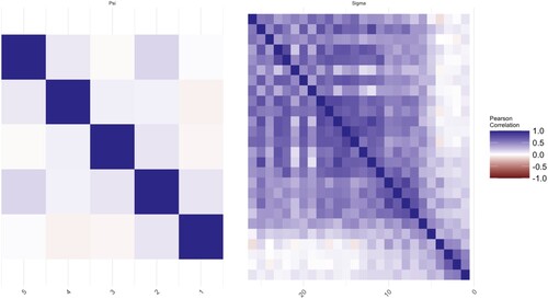
Each figure consists of two parts, the left-hand side is the plot of the elements in the matrix of ${\hat{\mathbf{\Psi }}}^{\ast }$. The right-hand side is the plot of $\hat{\mathbf{\Sigma }}$. The MLEs of the covariance matrices are given in Figures 2 and 3 as a benchmark. In Figure 2, there are some non-zero elements exist after a few empty elements in the off-diagonal areas, for example, the further upper-right area and lower-left area of $\hat{\mathbf{\Sigma }}$. This is the sparsity issue for longitudinal data. Intuitively, a further period implies a weaker connection between two-time points. For some practical needing, one would like to get rid of the effect of noises with long-term memory in the repeated measurements to reduce the bias of estimations. The same results can be observed from the MLEs of ${\hat{\mathbf{\Psi }}}^{\ast }$ as well. 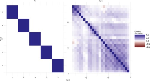The noises in $\hat{\mathbf{\Sigma }}$ at control groups are more obvious as we move from the diagonal to the upper-right and lower-left corners. The MCD-based estimations are given in Figures 4 and 5. The noises for both $\hat{\mathbf{\Sigma }}$ and ${\hat{\mathbf{\Psi }}}^{\ast }$ are shrunk and smoothed out on the further corners from the diagonal respectively. On the other hand, the information which is close to the diagonal is kept as shown in those figures.

Figure 3. Estimated correlation matrices for the control group using MLE.

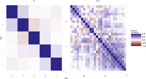
Figure 4. Estimated correlation matrices for the alcoholic group using the proposed method.

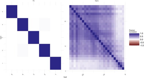
Figure 5. Estimated correlation matrices for the control group using the proposed method.

7. Conclusion

We propose a novel method to estimate Kronecker structured covariance matrix for matrix-valued data. The considered matrix is decomposed by MCD and each component from the decomposition is considered separately. Shrinkage and smoothing techniques are employed to take the typical features of the Cholesky factors into account and reduce the bias caused by the sparsity from large longitudinal data. The performance of RFF is illustrated by both simulations and empirical studies, which shows that the combination is useful. The theoretical results give the estimators' convergence rates and the upper bounds to the Kronecker product of components via MCD are derived.

The proposed approach is developed using MCD method which requires a pre-knowledge on the variable ordering. Natural ordering is typical for longitudinal data. When the situation arises that the variables do not have a natural ordering among themselves, this problem is of great interest and will be studied separately.

In this article we only study the Kronecker estimate for matrix-valued data. One possible extension is to consider the Kronecker covariance structure on array data, i.e. the Kronecker products of three or more components matrices, in this case model (5(5) $\mathrm{vec}{\mathbf{X}}_i\sim N_{pq}(\mathbf{0},\mathbf{\Psi }\otimes \mathbf{\Sigma }).$(5) ) becomes the array-normal distribution [30,31]. It is worthwhile to develop regularized methods further under this framework.

Acknowledgments

The authors thank the editor, the associate editor and two anonymous reviewers for their insightful comments which have resulted in significant improvement of this manuscript.

Disclosure statement

No potential conflict of interest was reported by the author(s).

Appendices

Appendix 1.

Some lemmas

Lemma A.1

Suppose that the eigenvalues of ${\mathbf{T}}_{1,0}$, ${\mathbf{T}}_{2,0}$, ${\mathbf{D}}_{1,0}$ and ${\mathbf{D}}_{2,0}$ are bounded by $d^{-1}$ and d, and that $pq/n\to [0,1)$. Consider $\Vert {\mathbf{T}}_1-{\mathbf{T}}_{1,0}{\Vert }_F^2=O(s_1{s}_2\log (pq)/n)$ and $\Vert {\mathbf{T}}_2-{\mathbf{T}}_{2,0}{\Vert }_F^2=O(s_1{s}_2\log (pq)/n)$, such that Assumption (C2) holds. Then, for any $ϵ>0$, there exists $C_{1,ϵ}$ and $C_{2,ϵ}$ such that $\begin{array}{rl}& P(\frac{1}{\sqrt{\log \left(pq\right)/n}}\underset{i,j}{max}\left|{\left\{({\mathbf{T}}_2\otimes {\mathbf{T}}_1)(\mathbf{S}-({\mathbf{\Psi }}_0\otimes {\mathbf{\Sigma }}_0)){({\mathbf{T}}_2\otimes {\mathbf{T}}_1)}^{\prime }\right\}}_{ij}\right|\le C_{1,ϵ})>1-ϵ,\\ & P(\frac{1}{\sqrt{\log \left(pq\right)/n}}\underset{i,j}{max}\left|{\left\{[\mathbf{S}-({\mathbf{\Psi }}_0\otimes {\mathbf{\Sigma }}_0)]{({\mathbf{T}}_{2,0}\otimes {\mathbf{T}}_{1,0})}^{\prime }({\mathbf{D}}_{2,0}^{-1}\otimes {\mathbf{D}}_{1,0}^{-1})\right\}}_{ij}\right|<C_{2,ϵ})>1-ϵ,\end{array}$for all $n\ge 1$.

Proof of Lemma A.1.

Since the eigenvalues of ${\mathbf{T}}_{1,0}$ and ${\mathbf{T}}_{2,0}$ are bounded, $\Vert {\mathbf{T}}_{2,0}\otimes {\mathbf{T}}_{1,0}\Vert$ is also bounded. Then, $\begin{array}{rl}& \Vert {\mathbf{T}}_2\otimes {\mathbf{T}}_1-{\mathbf{T}}_{2,0}\otimes {\mathbf{T}}_{1,0}\Vert =\Vert {\mathbf{T}}_{2,0}\otimes {\mathrm{\Delta }}_{\mathbf{T}}^{(1)}+{\mathrm{\Delta }}_{\mathbf{T}}^{(2)}\otimes {\mathbf{T}}_{1,0}+{\mathrm{\Delta }}_{\mathbf{T}}^{(2)}\otimes {\mathrm{\Delta }}_{\mathbf{T}}^{(1)}\Vert \\ & \le \Vert {\mathbf{T}}_{2,0}\otimes {\mathrm{\Delta }}_{\mathbf{T}}^{(1)}\Vert +\Vert {\mathrm{\Delta }}_{\mathbf{T}}^{(2)}\otimes {\mathbf{T}}_{1,0}\Vert +\Vert {\mathrm{\Delta }}_{\mathbf{T}}^{(2)}\otimes {\mathrm{\Delta }}_{\mathbf{T}}^{(1)}\Vert \\ & \le \Vert {\mathrm{\Delta }}_{\mathbf{T}}^{(1)}\Vert \Vert {\mathbf{T}}_{2,0}\Vert +\Vert {\mathbf{T}}_{1,0}\Vert \Vert {\mathrm{\Delta }}_{\mathbf{T}}^{(2)}\Vert +\Vert {\mathrm{\Delta }}_{\mathbf{T}}^{(1)}\Vert \Vert {\mathrm{\Delta }}_{\mathbf{T}}^{(2)}\Vert \\ & \le {\Vert {\mathrm{\Delta }}_{\mathbf{T}}^{(1)}\Vert }_F\Vert {\mathbf{T}}_{2,0}\Vert +\Vert {\mathbf{T}}_{1,0}\Vert {\Vert {\mathrm{\Delta }}_{\mathbf{T}}^{(2)}\Vert }_F+\Vert {\mathrm{\Delta }}_{\mathbf{T}}^{(1)}\Vert \Vert {\mathrm{\Delta }}_{\mathbf{T}}^{(2)}\Vert .\end{array}$By Assumption (C2), $\Vert {\mathbf{T}}_2\otimes {\mathbf{T}}_1-{\mathbf{T}}_{2,0}\otimes {\mathbf{T}}_{1,0}\Vert =o_P(1)$. Hence, by Lemma 3 in [32], we have $\underset{i,j}{max}\left|{\left\{({\mathbf{T}}_2\otimes {\mathbf{T}}_1)(\mathbf{S}-({\mathbf{\Psi }}_0\otimes {\mathbf{\Sigma }}_0)){({\mathbf{T}}_2\otimes {\mathbf{T}}_1)}^{\prime }\right\}}_{ij}\right|=O_P\left(\sqrt{\log \left(pq\right)/n}\right),$which establishes the first claim in this lemma.

Note that $\begin{array}{rl}& \underset{i,j}{max}\left|{\left\{[\mathbf{S}-({\mathbf{\Psi }}_0\otimes {\mathbf{\Sigma }}_0)]{({\mathbf{T}}_{2,0}\otimes {\mathbf{T}}_{1,0})}^{\prime }({\mathbf{D}}_{2,0}^{-1}\otimes {\mathbf{D}}_{1,0}^{-1})\right\}}_{ij}\right|\\ & =\underset{i,j}{max}\left|{\left\{({\mathbf{D}}_{2,0}^{-1}\otimes {\mathbf{D}}_{1,0}^{-1})({\mathbf{D}}_{2,0}\otimes {\mathbf{D}}_{1,0})[\mathbf{S}-({\mathbf{\Psi }}_0\otimes {\mathbf{\Sigma }}_0)]{({\mathbf{T}}_{2,0}\otimes {\mathbf{T}}_{1,0})}^{\prime }({\mathbf{D}}_{2,0}^{-1}\otimes {\mathbf{D}}_{1,0}^{-1})\right\}}_{ij}\right|\\ & =\underset{i,j}{max}\left|\frac{{\left\{({\mathbf{D}}_{2,0}\otimes {\mathbf{D}}_{1,0})[\mathbf{S}-({\mathbf{\Psi }}_0\otimes {\mathbf{\Sigma }}_0)]{({\mathbf{T}}_{2,0}\otimes {\mathbf{T}}_{1,0})}^{\prime }\right\}}_{ij}}{{({\mathbf{D}}_{2,0}\otimes {\mathbf{D}}_{1,0})}_{ii}{({\mathbf{D}}_{2,0}\otimes {\mathbf{D}}_{1,0})}_{jj}}\right|\\ & \le d^4\underset{i,j}{max}\left|{\left\{({\mathbf{D}}_{2,0}\otimes {\mathbf{D}}_{1,0})[\mathbf{S}-({\mathbf{\Psi }}_0\otimes {\mathbf{\Sigma }}_0)]{({\mathbf{T}}_{2,0}\otimes {\mathbf{T}}_{1,0})}^{\prime }\right\}}_{ij}\right|.\end{array}$Hence, by Lemma 3 in [32], we have $\underset{i,j}{max}\left|{\left\{({\mathbf{D}}_{2,0}\otimes {\mathbf{D}}_{1,0})[\mathbf{S}-({\mathbf{\Psi }}_0\otimes {\mathbf{\Sigma }}_0)]{({\mathbf{T}}_{2,0}\otimes {\mathbf{T}}_{1,0})}^{\prime }\right\}}_{ij}\right|=O_P\left(\sqrt{\log \left(pq\right)/n}\right).$Consequently, $\underset{ij}{max}\left|{\left\{[\mathbf{S}-({\mathbf{\Psi }}_0\otimes {\mathbf{\Sigma }}_0)]{[{\mathbf{T}}_{2,0}\otimes {\mathbf{T}}_{1,0}]}^{\prime }({\mathbf{D}}_{2,0}^{-1}\otimes {\mathbf{D}}_{1,0}^{-1})\right\}}_{ij}\right|\le d^4{O}_P\left(\sqrt{\log \left(pq\right)/n}\right),$which establishes the second claim in this lemma.

Lemma A.2

For the lower triangular matrices ${\mathbf{T}}_{2,0}$ and ${\mathbf{T}}_{1,0}$ in MCD, ${\Vert ({\mathbf{T}}_{2,0}+{\mathrm{\Delta }}_{\mathbf{T}}^{(2)})\otimes ({\mathbf{T}}_{1,0}+{\mathrm{\Delta }}_{\mathbf{T}}^{(1)})-{\mathbf{T}}_{2,0}\otimes {\mathbf{T}}_{2,0}\Vert }_F^2\ge q{\Vert {\mathrm{\Delta }}_{\mathbf{T}}^{(1)}\Vert }_F^2+p{\Vert {\mathrm{\Delta }}_{\mathbf{T}}^{(2)}\Vert }_F^2.$

Proof

Proof of Lemma A.2

Note that the diagonal entries of ${\mathbf{T}}_2$ and ${\mathbf{T}}_{2,0}$ are all 1's. Then, for $i=1,\dots ,q$, the $(i,i)$th block of $({\mathbf{T}}_{2,0}+{\mathrm{\Delta }}_{\mathbf{T}}^{(2)})\otimes ({\mathbf{T}}_{1,0}+{\mathrm{\Delta }}_{\mathbf{T}}^{(1)})-{\mathbf{T}}_{2,0}\otimes {\mathbf{T}}_{2,0}$ is simply ${\mathrm{\Delta }}_{\mathbf{T}}^{(1)}$. When $i\ne j$, the $(i,j)$th block matrix is ${\mathbf{T}}_{2,ij}({\mathbf{T}}_{1,0}+{\mathrm{\Delta }}_{\mathbf{T}}^{(1)})-{\mathbf{T}}_{2,0,ij}{\mathbf{T}}_{1,0}$. Its diagonal entries are all ${\mathbf{T}}_{2,ij}-{\mathbf{T}}_{2,0,ij}$, yielding $\Vert {\mathbf{T}}_{2,ij}({\mathbf{T}}_{1,0}+{\mathrm{\Delta }}_{\mathbf{T}}^{(1)})-{\mathbf{T}}_{2,0,ij}{\mathbf{T}}_{1,0}{\Vert }_F^2\ge p({\mathbf{T}}_{2,ij}-{\mathbf{T}}_{2,0,ij}{)}^2$. Hence, $\Vert ({\mathbf{T}}_{2,0}+{\mathrm{\Delta }}_{\mathbf{T}}^{(2)})\otimes ({\mathbf{T}}_{1,0}+{\mathrm{\Delta }}_{\mathbf{T}}^{(1)})-{\mathbf{T}}_{2,0}\otimes {\mathbf{T}}_{2,0}{\Vert }_F^2\ge \sum _{i=1}^q\Vert {\mathrm{\Delta }}_{\mathbf{T}}^{(1)}{\Vert }_F^2+\sum _{i\ne j}\Vert {\mathbf{T}}_{2,ij}({\mathbf{T}}_{1,0}+{\mathrm{\Delta }}_{\mathbf{T}}^{(1)})-{\mathbf{T}}_{2,0,ij}{\mathbf{T}}_{1,0}{\Vert }_F^2,$ which establishes the lemma.

Appendix 2.

Proof of Theorem 4.1

In this section, we will prove Theorem 4.1. Our proof by and large follows the steps in [28], but takes the MCD structure into account.

Under Assumption (C1), Lemma 2 of Jiang [28] implies that $\begin{array}{rl}& 0<1/d<{\psi }_{min}\left({\mathbf{T}}_{i,0}\right)\le {\psi }_{max}\left({\mathbf{T}}_{i,0}\right)<d<\mathrm{\infty },\\ & 0<1/d<{\lambda }_{min}\left({\mathbf{D}}_{i,0}\right)\le {\lambda }_{max}\left({\mathbf{D}}_{i,0}\right)<d<\mathrm{\infty },\end{array}$for i = 1, 2, where $\psi (.)$ denotes the singular value of $\mathbf{T}$. Set ${\mathbf{E}}_i={\mathbf{D}}_i^{-1}$, ${\mathbf{E}}_{i,0}={\mathbf{D}}_{i,0}^{-1}$, i = 1, 2. Since the eigenvalues of ${\mathbf{D}}_{i,0}$ are bounded, we also have $0<1/d<{\lambda }_{min}\left({\mathbf{E}}_{i,0}\right)\le {\lambda }_{max}\left({\mathbf{E}}_{i,0}\right)<d<\mathrm{\infty }.$Let $\log L({\mathbf{D}}_1,{\mathbf{T}}_1,{\mathbf{D}}_2,{\mathbf{T}}_2)$ be the log-likelihood, and $G({\mathrm{\Delta }}_{\mathbf{D}}^{(1)},{\mathrm{\Delta }}_{\mathbf{T}}^{(1)},{\mathrm{\Delta }}_{\mathbf{D}}^{(2)},{\mathrm{\Delta }}_{\mathbf{T}}^{(2)})$ be $-2$ times the difference between the penalized likelihood function of the estimated covariance matrix and the true covariance matrix, where ${\mathbf{D}}_1={\mathbf{D}}_{1,0}+{\mathrm{\Delta }}_{\mathbf{D}}^{(1)}$, ${\mathbf{T}}_1={\mathbf{T}}_{1,0}+{\mathrm{\Delta }}_{\mathbf{T}}^{(1)}$, ${\mathbf{D}}_2={\mathbf{D}}_{2,0}+{\mathrm{\Delta }}_{\mathbf{D}}^{(2)}$, and ${\mathbf{T}}_2={\mathbf{T}}_{2,0}+{\mathrm{\Delta }}_{\mathbf{T}}^{(2)}$. Consider ${\mathcal{A}}_1=\{{\mathrm{\Delta }}_{\mathbf{T}}^{(1)}:\Vert {\mathrm{\Delta }}_{\mathbf{T}}^{(1)}{\Vert }_F^2\le U_1^2{s}_1{s}_2\log (pq)/n\}$, ${\mathcal{A}}_2=\{{\mathrm{\Delta }}_{\mathbf{T}}^{(2)}:\Vert {\mathrm{\Delta }}_{\mathbf{T}}^{(1)}{\Vert }_F^2\le U_2^2{s}_1{s}_2\log (pq)/n\}$, ${\mathcal{B}}_1=\{{\mathrm{\Delta }}_{\mathbf{D}}^{(1)}:\Vert {\mathrm{\Delta }}_{\mathbf{D}}^{(1)}{\Vert }_F^2\le V_1^{2}p\log (pq)/n\}$, and ${\mathcal{B}}_2=\{{\mathrm{\Delta }}_{\mathbf{D}}^{(2)}:\Vert {\mathrm{\Delta }}_{\mathbf{D}}^{(2)}{\Vert }_F^2\le V_2^{2}q\log (pq)/n\}$. We will show that, for every ${\mathrm{\Delta }}_{\mathbf{T}}^{(1)}$, ${\mathrm{\Delta }}_{\mathbf{T}}^{(2)}$, ${\mathrm{\Delta }}_{\mathbf{D}}^{(1)}$, and ${\mathrm{\Delta }}_{\mathbf{D}}^{(2)}$ at the boundaries of respective ${\mathcal{A}}_1$, ${\mathcal{A}}_2$, ${\mathcal{B}}_1$, and ${\mathcal{B}}_2$, the probability $P(G({\mathrm{\Delta }}_{\mathbf{D}}^{(1)},{\mathrm{\Delta }}_{\mathbf{T}}^{(1)},{\mathrm{\Delta }}_{\mathbf{D}}^{(2)},{\mathrm{\Delta }}_{\mathbf{T}}^{(2)}))>0$ tends to 1 for sufficiently large $U_1,U_2$ and $V_1,V_2$.

Define ${\mathrm{\Delta }}_{\mathbf{E}}^{(1,2)}={\mathbf{E}}_2\otimes {\mathbf{E}}_1-{\mathbf{E}}_{2,0}\otimes {\mathbf{E}}_{1,0}$, ${\mathrm{\Delta }}_{\mathbf{T}}^{(1,2)}={\mathbf{T}}_2\otimes {\mathbf{T}}_1-{\mathbf{T}}_{2,0}\otimes {\mathbf{T}}_{1,0}$, and ${\mathrm{\Delta }}_{\mathbf{D}}^{(1,2)}={\mathbf{D}}_2\otimes {\mathbf{D}}_1-{\mathbf{D}}_{2,0}\otimes {\mathbf{D}}_{1,0}$. Let $\mathbf{S}$ be the sample covariance matrix of size $pq\times pq$. Then, $-2$ times the difference between the unpenalized likelihood function of the estimated covariance matrix and the true covariance matrix can be expressed as $\begin{array}{rl}& -2(\log L({\mathbf{D}}_1,{\mathbf{T}}_1,{\mathbf{D}}_2,{\mathbf{T}}_2)-\log L({\mathbf{D}}_{1,0},{\mathbf{T}}_{1,0},{\mathbf{D}}_{2,0},{\mathbf{T}}_{2,0}))\\ & =\log |{\mathbf{D}}_2\otimes {\mathbf{D}}_1|+tr\left\{\mathbf{S}{({\mathbf{T}}_2\otimes {\mathbf{T}}_1)}^{\prime }({\mathbf{D}}_2^{-1}\otimes {\mathbf{D}}_1^{-1})({\mathbf{T}}_2\otimes {\mathbf{T}}_1)\right\}-\log |{\mathbf{D}}_{2,0}\otimes {\mathbf{D}}_{1,0}|\\ & -tr\left\{\mathbf{S}{({\mathbf{T}}_{2,0}\otimes {\mathbf{T}}_{1,0})}^{\prime }({\mathbf{D}}_{2,0}^{-1}\otimes {\mathbf{D}}_{1,0}^{-1})({\mathbf{T}}_{2,0}\otimes {\mathbf{T}}_{1,0})\right\}\\ & =-tr\left\{{[{\mathbf{E}}_{2,0}\otimes {\mathbf{E}}_{1,0}]}^{-1}{\mathrm{\Delta }}_{\mathbf{E}}^{(1,2)}\right\}\\ & +\underset{0}{\overset{1}{\int }}(1-v)ve{c}^{\prime }\left({\mathrm{\Delta }}_{\mathbf{E}}^{(1,2)}\right){[{\mathbf{E}}_{2,0}\otimes {\mathbf{E}}_{1,0}+v{\mathrm{\Delta }}_{\mathbf{E}}^{(1,2)}]}^{\otimes -2}vec\left({\mathrm{\Delta }}_{\mathbf{E}}^{(1,2)}\right)\mathrm{d}v\\ & +tr\left\{\mathbf{S}{({\mathbf{T}}_2\otimes {\mathbf{T}}_1)}^{\prime }({\mathbf{D}}_2^{-1}\otimes {\mathbf{D}}_1^{-1})({\mathbf{T}}_2\otimes {\mathbf{T}}_1)\right\}\\ & -tr\left\{\mathbf{S}{({\mathbf{T}}_{2,0}\otimes {\mathbf{T}}_{1,0})}^{\prime }({\mathbf{D}}_{2,0}^{-1}\otimes {\mathbf{D}}_{1,0}^{-1})({\mathbf{T}}_{2,0}\otimes {\mathbf{T}}_{1,0})\right\}\\ & =\underset{0}{\overset{1}{\int }}(1-v)ve{c}^{\prime }\left({\mathrm{\Delta }}_{\mathbf{E}}^{(1,2)}\right){[{\mathbf{E}}_{2,0}\otimes {\mathbf{E}}_{1,0}+v{\mathrm{\Delta }}_{\mathbf{E}}^{(1,2)}]}^{\otimes -2}vec\left({\mathrm{\Delta }}_{\mathbf{E}}^{(1,2)}\right)\mathrm{d}v\\ & -tr\left\{[{\mathbf{D}}_{2,0}\otimes {\mathbf{D}}_{1,0}]{\mathbf{\Delta }}_E^{(1,2)}\right\}\\ & +tr\left\{\mathbf{S}{({\mathbf{T}}_2\otimes {\mathbf{T}}_1)}^{\prime }({\mathbf{D}}_2^{-1}\otimes {\mathbf{D}}_1^{-1})({\mathbf{T}}_2\otimes {\mathbf{T}}_1)\right\}\\ & -tr\left\{\mathbf{S}{({\mathbf{T}}_{2,0}\otimes {\mathbf{T}}_{1,0})}^{\prime }({\mathbf{D}}_{2,0}^{-1}\otimes {\mathbf{D}}_{1,0}^{-1})({\mathbf{T}}_{2,0}\otimes {\mathbf{T}}_{1,0})\right\},\end{array}$where we have used Taylor expansion with the integral form of the remainder in the second equality.

We can partition $G({\mathrm{\Delta }}_{\mathbf{D}}^{(1)},{\mathrm{\Delta }}_{\mathbf{T}}^{(1)},{\mathrm{\Delta }}_{\mathbf{D}}^{(2)},{\mathrm{\Delta }}_{\mathbf{T}}^{(2)})$ as $G({\mathrm{\Delta }}_{\mathbf{D}}^{(1)},{\mathrm{\Delta }}_{\mathbf{T}}^{(1)},{\mathrm{\Delta }}_{\mathbf{D}}^{(2)},{\mathrm{\Delta }}_{\mathbf{T}}^{(2)})=M_1+M_2+M_3+S_1+S_2+S_3,$where $\begin{array}{rl}{M}_1& =\underset{0}{\overset{1}{\int }}(1-v)ve{c}^{\prime }\left({\mathrm{\Delta }}_{\mathbf{E}}^{(1,2)}\right){[{\mathbf{E}}_{2,0}\otimes {\mathbf{E}}_{1,0}+v{\mathrm{\Delta }}_{\mathbf{E}}^{(1,2)}]}^{\otimes -2}vec\left({\mathrm{\Delta }}_{\mathbf{E}}^{(1,2)}\right)\mathrm{d}v,\\ M_2& =tr\left\{{\mathrm{\Delta }}_{\mathbf{E}}^{(1,2)}({\mathbf{T}}_2\otimes {\mathbf{T}}_1)(\mathbf{S}-{\mathbf{\Psi }}_0\otimes {\mathbf{\Sigma }}_0){({\mathbf{T}}_2\otimes {\mathbf{T}}_1)}^{\prime }\right\},\\ M_3& =tr\left\{({\mathbf{D}}_{2,0}^{-1}\otimes {\mathbf{D}}_{1,0}^{-1})[({\mathbf{T}}_2\otimes {\mathbf{T}}_1)\mathbf{S}{({\mathbf{T}}_2\otimes {\mathbf{T}}_1)}^{\prime }-({\mathbf{T}}_{2,0}\otimes {\mathbf{T}}_{1,0})\mathbf{S}{({\mathbf{T}}_{2,0}\otimes {\mathbf{T}}_{1,0})}^{\prime }]\right\}\\ & +tr\left\{{\mathrm{\Delta }}_{\mathbf{E}}^{(1,2)}({\mathbf{T}}_2\otimes {\mathbf{T}}_1)({\mathbf{\Psi }}_0\otimes {\mathbf{\Sigma }}_0){({\mathbf{T}}_2\otimes {\mathbf{T}}_1)}^{\prime }\right\}-tr\left\{({\mathbf{D}}_{2,0}\otimes {\mathbf{D}}_{1,0}){\mathrm{\Delta }}_{\mathbf{E}}^{(1,2)}\right\},\\ S_1& ={\lambda }_{sh,1}\sum _{t=2}^p\sum _{k=1}^{t-1}\left|{\mathbf{T}}_{1,tk}\right|+{\lambda }_{sh,2}\sum _{s=2}^q\sum _{k=1}^{s-1}\left|{\mathbf{T}}_{2,sk}\right|-{\lambda }_{sh,1}\sum _{t=2}^p\sum _{k=1}^{t-1}\left|{\mathbf{T}}_{1,tk,0}\right|-{\lambda }_{sh,2}\sum _{s=2}^q\sum _{k=1}^{s-1}\left|{\mathbf{T}}_{2,sk,0}\right|,\\ S_2& ={\lambda }_{sm,1}\sum _{t=2}^{p-2}\sum _{j=1}^{t-1}{[({\varphi }_{t+2,t+2-j}-{\varphi }_{t+1,t+1-j})-({\varphi }_{t+1,t+1-j}-{\varphi }_{t,t-j})]}^2\\ & -{\lambda }_{sm,1}\sum _{t=2}^{p-2}\sum _{j=1}^{t-1}{[({\varphi }_{t+2,t+2-j,0}-{\varphi }_{t+1,t+1-j,0})-({\varphi }_{t+1,t+1-j}-{\varphi }_{t,t-j,0})]}^2,\\ S_3& ={\lambda }_{sm,2}\sum _{s=2}^{q-2}\sum _{k=1}^{s-1}{[({\eta }_{s+2,s+2-k}-{\eta }_{s+1,s+1-k})-({\eta }_{s+1,s+1-k}-{\eta }_{s,s-k})]}^2\\ & -{\lambda }_{sm,2}\sum _{s=2}^{q-2}\sum _{k=1}^{s-1}{[({\eta }_{s+2,s+2-k,0}-{\eta }_{s+1,s+1-k,0})-({\eta }_{s+1,s+1-k,0}-{\eta }_{s,s-k,0})]}^2.\end{array}$We consider these terms separately.

A2.1. The term $M_1$

Using triangular inequality, we have $\Vert {\mathbf{E}}_{2,0}\otimes {\mathbf{E}}_{1,0}+v{\mathrm{\Delta }}_{\mathbf{E}}^{(1,2)}\Vert \le \Vert {\mathbf{E}}_{2,0}\otimes {\mathbf{E}}_{1,0}\Vert +v\Vert {\mathrm{\Delta }}_{\mathbf{E}}^{(1,2)}\Vert ,$ where $\Vert {\mathrm{\Delta }}_{\mathbf{E}}^{(1,2)}{\Vert }_F=o(1)$ by Assumption (C3). Since $\Vert {\mathbf{E}}_{2,0}\otimes {\mathbf{E}}_{1,0}\Vert$ is bounded from above and below, for a sufficiently large n, $v\Vert {\mathrm{\Delta }}_{\mathbf{E}}^{(1,2)}\Vert$ is dominated by $\Vert {\mathbf{E}}_{2,0}\otimes {\mathbf{E}}_{1,0}\Vert$ for any $v\in [0,1]$. That is saying, (A1) $\Vert {\mathbf{E}}_{2,0}\otimes {\mathbf{E}}_{1,0}+v{\mathrm{\Delta }}_{\mathbf{E}}^{(1,2)}\Vert \le \Vert {\mathbf{E}}_{2,0}\otimes {\mathbf{E}}_{1,0}\Vert +v\Vert {\mathrm{\Delta }}_{\mathbf{E}}^{(1,2)}\Vert \le 2\Vert {\mathbf{E}}_{2,0}\otimes {\mathbf{E}}_{1,0}\Vert \le 2d^2.$(A1) Therefore, we have $\begin{array}{rl}{M}_1& \ge \underset{0}{\overset{1}{\int }}(1-v){\lambda }_{min}\left\{{[{\mathbf{E}}_{2,0}\otimes {\mathbf{E}}_{1,0}+v{\mathrm{\Delta }}_{\mathbf{E}}^{(1,2)}]}^{\otimes -2}\right\}ve{c}^{\prime }\left({\mathrm{\Delta }}_{\mathbf{E}}^{(1,2)}\right)vec\left({\mathrm{\Delta }}_{\mathbf{E}}^{(1,2)}\right)\mathrm{d}v\\ & \ge \underset{0}{\overset{1}{\int }}(1-v){\lambda }_{min}\left\{{[{\mathbf{E}}_{2,0}\otimes {\mathbf{E}}_{1,0}+v{\mathrm{\Delta }}_{\mathbf{E}}^{(1,2)}]}^{\otimes -2}\right\}{\Vert vec\left({\mathrm{\Delta }}_{\mathbf{E}}^{(1,2)}\right)\Vert }_2^2\mathrm{d}v\\ & =\underset{0}{\overset{1}{\int }}(1-v){\Vert {\mathbf{E}}_{2,0}\otimes {\mathbf{E}}_{1,0}+v{\mathrm{\Delta }}_{\mathbf{E}}^{(1,2)}\Vert }^{-2}{\Vert {\mathrm{\Delta }}_{\mathbf{E}}^{(1,2)}\Vert }_F^2\mathrm{d}v\ge \frac{1}{8d^4}{\Vert {\mathrm{\Delta }}_{\mathbf{E}}^{(1,2)}\Vert }_F^2,\end{array}$where the last inequality holds because of (A1(A1) $\Vert {\mathbf{E}}_{2,0}\otimes {\mathbf{E}}_{1,0}+v{\mathrm{\Delta }}_{\mathbf{E}}^{(1,2)}\Vert \le \Vert {\mathbf{E}}_{2,0}\otimes {\mathbf{E}}_{1,0}\Vert +v\Vert {\mathrm{\Delta }}_{\mathbf{E}}^{(1,2)}\Vert \le 2\Vert {\mathbf{E}}_{2,0}\otimes {\mathbf{E}}_{1,0}\Vert \le 2d^2.$(A1) ). It is straightforward to see that (A2) $\begin{array}{rl}{\Vert {\mathrm{\Delta }}_{\mathbf{E}}^{(1,2)}\Vert }_F^2& =\sum _{i,j}{(\frac{1}{{\sigma }_i^2{\gamma }_j^2}-\frac{1}{{\sigma }_{i,0}^2{\gamma }_{j,0}^2})}^2=\sum _{i,j}{\left(\frac{{\sigma }_{i,0}^2{\gamma }_{j,0}^2-{\sigma }_i^2{\gamma }_j^2}{{\sigma }_i^2{\gamma }_j^2{\sigma }_{i,0}^2{\gamma }_{j,0}^2}\right)}^2\\ & \ge d^{-4}\sum _{i,j}{({\sigma }_{i,0}^2{\gamma }_{j,0}^2-{\sigma }_i^2{\gamma }_j^2)}^2=d^{-4}{\Vert {\mathrm{\Delta }}_{\mathbf{D}}^{(1,2)}\Vert }_F^2,\end{array}$(A2) where ${\sigma }_i^2$ is the ith diagonal element of ${\mathbf{D}}_1$, ${\gamma }_j^2$ is the jth diagonal element of ${\mathbf{D}}_2$, and the subscript ‘0’ indicates the true value of the element. Hence $M_1\ge \Vert {\mathrm{\Delta }}_{\mathbf{D}}^{(1,2)}{\Vert }_F^2/(8d^8)$.

A2.2. The term $M_2$

For $M_2$, $\begin{array}{rl}\left|M_2\right|& =\left|tr\left\{{\mathrm{\Delta }}_{\mathbf{E}}^{(1,2)}({\mathbf{T}}_2\otimes {\mathbf{T}}_1)(\mathbf{S}-{\mathbf{\Psi }}_0\otimes {\mathbf{\Sigma }}_0){({\mathbf{T}}_2\otimes {\mathbf{T}}_1)}^{\prime }\right\}\right|\\ & =\left|\sum _{i=1}^{pq}{\mathrm{\Delta }}_{\mathbf{E},i}^{(1,2)}{\left[({\mathbf{T}}_2\otimes {\mathbf{T}}_1)(\mathbf{S}-{\mathbf{\Psi }}_0\otimes {\mathbf{\Sigma }}_0){({\mathbf{T}}_2\otimes {\mathbf{T}}_1)}^{\prime }\right]}_{ii}\right|\\ & \le \left(\underset{i,j}{max}\left|{\left[({\mathbf{T}}_2\otimes {\mathbf{T}}_1)(\mathbf{S}-{\mathbf{\Psi }}_0\otimes {\mathbf{\Sigma }}_0){({\mathbf{T}}_2\otimes {\mathbf{T}}_1)}^{\prime }\right]}_{ij}\right|\right)\left(\sum _i\left|{\mathrm{\Delta }}_{\mathbf{E},i}^{(1,2)}\right|\right).\end{array}$By Lemma A.1, for a sufficiently large n, there exists a $C_{1,ϵ}$ such that $\begin{array}{rl}1-ϵ& <P(\frac{1}{\sqrt{\log \left(pq\right)/n}}\left|M_2\right|\le \sum _i\left|{\mathrm{\Delta }}_{\mathbf{E},i}^{(1,2)}\right|C_{1,ϵ})\\ & \le P(\left|M_2\right|\le d^4{\Vert {\mathrm{\Delta }}_{\mathbf{D}}^{(1,2)}\Vert }_F\sqrt{pq\log \left(pq\right)/n}{C}_{1,ϵ}),\end{array}$where the second inequality holds since $\sum _i\left|{\mathrm{\Delta }}_{{\mathbf{E}}_i}^{(1,2)}\right|\le \sqrt{pq}{\Vert {\mathrm{\Delta }}_{\mathbf{E}}^{(1,2)}\Vert }_F\le d^2\sqrt{pq}{\Vert {\mathrm{\Delta }}_{\mathbf{D}}^{(1,2)}\Vert }_F.$

A2.3. The term $M_3$

$M_3$ can be partitioned into $L_1+L_2+L_3$, where $\begin{array}{rl}{L}_1& =tr\left\{({\mathbf{D}}_{2,0}^{-1}\otimes {\mathbf{D}}_{1,0}^{-1})({\mathbf{T}}_{2,0}\otimes {\mathbf{T}}_{1,0})[\mathbf{S}-{\mathbf{\Psi }}_0\otimes {\mathbf{\Sigma }}_0]{\left({\mathrm{\Delta }}_{\mathbf{T}}^{(1,2)}\right)}^{\prime }\right\}\\ & +tr\left\{({\mathbf{D}}_{2,0}^{-1}\otimes {\mathbf{D}}_{1,0}^{-1}){\mathrm{\Delta }}_{\mathbf{T}}^{(1,2)}[\mathbf{S}-{\mathbf{\Psi }}_0\otimes {\mathbf{\Sigma }}_0]{({\mathbf{T}}_{2,0}\otimes {\mathbf{T}}_{1,0})}^{\prime }\right\},\\ L_2& =tr\left\{({\mathbf{D}}_{2,0}^{-1}\otimes {\mathbf{D}}_{1,0}^{-1}){\mathrm{\Delta }}_{\mathbf{T}}^{(1,2)}[\mathbf{S}-{\mathbf{\Psi }}_0\otimes {\mathbf{\Sigma }}_0]{\left({\mathrm{\Delta }}_{\mathbf{T}}^{(1,2)}\right)}^{\prime }\right\},\\ L_3& =tr\left\{({\mathbf{D}}_2^{-1}\otimes {\mathbf{D}}_1^{-1}){\mathrm{\Delta }}_{\mathbf{T}}^{(1,2)}({\mathbf{\Psi }}_0\otimes {\mathbf{\Sigma }}_0){\left({\mathrm{\Delta }}_{\mathbf{T}}^{(1,2)}\right)}^{\prime }\right\}.\end{array}$We will consider $L_1$, $L_2$, and $L_3$ separately. For $L_1$, $\begin{array}{rl}\left|L_1\right|& \le \left|tr({\mathbf{D}}_{2,0}^{-1}\otimes {\mathbf{D}}_{1,0}^{-1})({\mathbf{T}}_{2,0}\otimes {\mathbf{T}}_{1,0})[\mathbf{S}-{\mathbf{\Psi }}_0\otimes {\mathbf{\Sigma }}_0]{\left({\mathrm{\Delta }}_{\mathbf{T}}^{(1,2)}\right)}^{\prime }\right|\\ & +\left|tr\left\{({\mathbf{D}}_{2,0}^{-1}\otimes {\mathbf{D}}_{1,0}^{-1}){\mathrm{\Delta }}_{\mathbf{T}}^{(1,2)}[\mathbf{S}-{\mathbf{\Psi }}_0\otimes {\mathbf{\Sigma }}_0]{({\mathbf{T}}_{2,0}\otimes {\mathbf{T}}_{1,0})}^{\prime }\right\}\right|\\ & =2\left|tr\left\{({\mathbf{D}}_{2,0}^{-1}\otimes {\mathbf{D}}_{1,0}^{-1}){\mathrm{\Delta }}_{\mathbf{T}}^{(1,2)}[\mathbf{S}-{\mathbf{\Psi }}_0\otimes {\mathbf{\Sigma }}_0]{({\mathbf{T}}_{2,0}\otimes {\mathbf{T}}_{1,0})}^{\prime }\right\}\right|\\ & =2\left|\sum _{i,j}{\mathrm{\Delta }}_{\mathbf{T},ij}^{(1,2)}{\left[(\mathbf{S}-{\mathbf{\Psi }}_0\otimes {\mathbf{\Sigma }}_0){({\mathbf{T}}_{2,0}\otimes {\mathbf{T}}_{1,0})}^{\prime }({\mathbf{D}}_{2,0}^{-1}\otimes {\mathbf{D}}_{1,0}^{-1})\right]}_{ji}\right|\\ & \le 2\left(\sum _{i,j}\left|{\mathrm{\Delta }}_{\mathbf{T},ij}^{(1,2)}\right|\right)\underset{i,j}{max}\left|{\left[(\mathbf{S}-{\mathbf{\Psi }}_0\otimes {\mathbf{\Sigma }}_0){({\mathbf{T}}_{2,0}\otimes {\mathbf{T}}_{1,0})}^{\prime }({\mathbf{D}}_{2,0}^{-1}\otimes {\mathbf{D}}_{1,0}^{-1})\right]}_{ji}\right|.\end{array}$Hence, by Lemma A.1, for a sufficiently large n, there exists a $C_{2,ϵ}$ such that with probability greater than $1-ϵ$ we have $\left|L_1\right|\le 2\left(\sum _{i,j}\left|{\mathrm{\Delta }}_{\mathbf{T},ij}^{(1,2)}\right|\right)\sqrt{\log \left(pq\right)/n}{C}_{2,ϵ}.$Let $Z_i=\{j,k\}$ be the set of indices such that ${\mathbf{T}}_{i,jk,0}$ is nonzero. Then, with a probability of greater than $1-ϵ$, $\begin{array}{r}\left|L_1\right|\le 2\left(\sum _{\begin{array}{c}ij\in Z_1^C\\ \mathrm{or}\\ sk\in Z_2^C\end{array}}\left|{\mathbf{T}}_{1,ij}\right|\left|{\mathbf{T}}_{2,sk}\right|\right)\sqrt{\log \left(pq\right)/n}{C}_{2,ϵ}+2\sqrt{s_1{s}_2}{\Vert {\mathrm{\Delta }}_{\mathbf{T}}^{(1,2)}\Vert }_F\sqrt{\log \left(pq\right)/n}{C}_{2,ϵ}.\end{array}$For $L_2$, $\begin{array}{rl}\left|L_2\right|& =\left|ve{c}^{\mathrm{\prime }}\left[{\mathrm{\Delta }}_{\mathbf{T}}^{(1,2)}\right]\{[\mathbf{S}-{\mathbf{\Psi }}_0\otimes {\mathbf{\Sigma }}_0]\otimes {\mathbf{D}}_{2,0}^{-1}\otimes {\mathbf{D}}_{1,0}^{-1}\}vec\left[{\mathrm{\Delta }}_{\mathbf{T}}^{(1,2)}\right]\right|\\ & \le \Vert [\mathbf{S}-{\mathbf{\Psi }}_0\otimes {\mathbf{\Sigma }}_0]\otimes ({\mathbf{D}}_{2,0}^{-1}\otimes {\mathbf{D}}_{1,0}^{-1})\Vert {\Vert {\mathrm{\Delta }}_{\mathbf{T}}^{(1,2)}\Vert }_F^2,\end{array}$where the inequality holds from the result that the maximum value of ${\mathbf{x}}^{\prime }\mathbf{A}\mathbf{x}$ with a symmetric matrix $\mathbf{A}$ and a unit vector $\mathbf{x}$ is ${\lambda }_{max}(\mathbf{A})$. Hence, $\left|L_2\right|\le \Vert \mathbf{S}-{\mathbf{\Psi }}_0\otimes {\mathbf{\Sigma }}_0\Vert \Vert {\mathbf{D}}_{2,0}^{-1}\otimes {\mathbf{D}}_{1,0}^{-1}\Vert {\Vert {\mathrm{\Delta }}_{\mathbf{T}}^{(1,2)}\Vert }_F^2=o_P\left(1\right){\Vert {\mathrm{\Delta }}_{\mathbf{T}}^{(1,2)}\Vert }_F^2,$where the equality holds since the proof of Lemma 3 in [32] shows that $\Vert \mathbf{S}-({\mathbf{\Psi }}_0\otimes {\mathbf{\Sigma }}_0)\Vert =o_P(1)$. For $L_3$, $\begin{array}{rl}{L}_3& =ve{c}^{\prime }\left({\mathrm{\Delta }}_{\mathbf{T}}^{(1,2)}\right)[{\mathbf{\Psi }}_0\otimes {\mathbf{\Sigma }}_0\otimes {\mathbf{D}}_2^{-1}\otimes {\mathbf{D}}_1^{-1}]vec\left({\mathrm{\Delta }}_{\mathbf{T}}^{(1,2)}\right)\\ & \ge {\lambda }_{min}({\mathbf{\Psi }}_0\otimes {\mathbf{\Sigma }}_0){\lambda }_{min}({\mathbf{D}}_2^{-1}\otimes {\mathbf{D}}_1^{-1}){\Vert {\mathrm{\Delta }}_{\mathbf{T}}^{(1,2)}\Vert }_F^2=\frac{1}{d^4}{\Vert {\mathrm{\Delta }}_{\mathbf{T}}^{(1,2)}\Vert }_F^2,\end{array}$where the inequality holds from the result that the minimum value of ${\mathbf{x}}^{\prime }\mathbf{A}\mathbf{x}$ with a symmetric matrix $\mathbf{A}$ and a unit vector $\mathbf{x}$ is ${\lambda }_{min}(\mathbf{A})$. Hence, $L_2$ is dominated by $L_3$, such that $L_3-|L_2|>0$ for a sufficiently large n.

A2.3.1. The shrinkage penalty term

The shrinkage penalty term is $S_1=Q_1+Q_2+Q_3$, where $Q_1={\lambda }_{sh,1}\sum _{t,k\in Z_1^c}|{\mathbf{T}}_{1,tk}|+{\lambda }_{sh,2}\sum _{s,k\in Z_2^c}|{\mathbf{T}}_{2,sk}|,Q_2={\lambda }_{sh,1}\sum _{t,k\in Z_1}|{\mathbf{T}}_{1,tk}|-{\lambda }_{sh,1}\sum _{t,k\in Z_1}|{\mathbf{T}}_{1,tk,0}|$ and $Q_3={\lambda }_{sh,2}\sum _{s,k\in Z_2}|{\mathbf{T}}_{2,sk}|-{\lambda }_{sh,2}\sum _{s,k\in Z_1}|{\mathbf{T}}_{2,sk,0}|$. It is easy to see that $Q_1>0$. For $Q_2$, $|Q_2|\le {\lambda }_{sh,1}\sum _{t,k\in Z_1}\Vert {\mathbf{T}}_{1,tk}|-|{\mathbf{T}}_{1,tk,0}\Vert \le {\lambda }_{sh,1}\sum _{t,k\in Z_1}|{\mathbf{T}}_{1,tk}-{\mathbf{T}}_{1,tk,0}|\le {\lambda }_{sh,1}\sqrt{s_1}\Vert {\mathrm{\Delta }}_{\mathbf{T}}^{(1)}{\Vert }_F$. Likewise, $|Q_3|\le {\lambda }_{sh,2}\sqrt{s_2}\Vert {\mathrm{\Delta }}_{\mathbf{T}}^{(2)}{\Vert }_F$.

A2.3.2. The smoothing penalty term

Let $A_{tj}={\varphi }_{t+2,t+2-j}-{\varphi }_{t+1,t+1-j}$ be the difference between two neighbouring elements on the off-diagonal of $\mathbf{T}$. Likewise, let $B_{tj}={\varphi }_{t+1,t+1-j}-{\varphi }_{t,t-j}$, $A_{tj,0}={\varphi }_{t+2,t+2-j,0}-{\varphi }_{t+1,t+1-j,0}$ and $B_{tj,0}={\varphi }_{t+1,t+1-j,0}-{\varphi }_{t,t-j,0}$. Then, (A3) $\begin{array}{rl}\left|S_2\right|& ={\lambda }_{sm}\sum _{t,j}\left|(A_{tj}-B_{tj}-A_{tj,0}+B_{tj,0})(A_{tj}-B_{tj}+A_{tj,0}-B_{tj,0})\right|\\ & \le {\lambda }_{sm}\sqrt{\sum _{t,j}{|A_{tj}-B_{tj}-A_{tj,0}+B_{tj,0}|}^2}\sqrt{\sum _{t,j}{|A_{tj}-B_{tj}+A_{tj,0}-B_{tj,0}|}^2}\\ & \le \frac{{\lambda }_{sm}}{2}[\sum _{t,j}{|A_{tj}-B_{tj}-A_{tj,0}+B_{tj,0}|}^2+\sum _{t,j}{|A_{tj}-B_{tj}+A_{tj,0}-B_{tj,0}|}^2]\\ & \le \frac{{\lambda }_{sm}}{2}\sum _{t,j}[3{|A_{tj}-A_{tj,0}-(B_{tj}-B_{tj,0})|}^2+8{|A_{tj,0}-B_{tj,0}|}^2],\end{array}$(A3) where the last inequality holds since $\begin{array}{rl}{|A_{tj}-B_{tj}+A_{tj,0}-B_{tj,0}|}^2& ={|A_{tj}-A_{tj,0}-(B_{tj}-B_{tj,0})+2(A_{tj,0}-B_{tj,0})|}^2\\ & \le 2{|A_{tj}-A_{tj,0}-(B_{tj}-B_{tj,0})|}^2+8{(A_{tj,0}-B_{tj,0})}^2.\end{array}$Note, $\begin{array}{rl}& \sum _{t,j}{|A_{tj}-A_{tj,0}|}^2\le \sum _{t,j}{|{\varphi }_{t+2,t+2-j}-{\varphi }_{t+2,t+2-j,0}|}^2\\ & +2\sum _{t,j}|{\varphi }_{t+2,t+2-j}-{\varphi }_{t+2,t+2-j,0}||{\varphi }_{t+1,t+1-j}-{\varphi }_{t+1,t+1-j,0}|\\ & +\sum _{t,j}{|{\varphi }_{t+1,t+1-j}-{\varphi }_{t+1,t+1-j,0}|}^2\\ & \le 2\Vert {\mathrm{\Delta }}_{\mathbf{T}}{\Vert }_F^2+2\sum _{t,j}|{\varphi }_{t+2,t+2-j}-{\varphi }_{t+2,t+2-j,0}||{\varphi }_{t+1,t+1-j}-{\varphi }_{t+1,t+1-j,0}|\le 4\Vert {\mathrm{\Delta }}_{\mathbf{T}}{\Vert }_F^2.\end{array}$Likewise, $\sum _{t,j}|B_{tj}-B_{tj,0}{|}^2\le 4\Vert {\mathrm{\Delta }}_{\mathbf{T}}{\Vert }_F^2$. By Cauchy-Schwarz inequality, $\sum _{t,j}|A_{tj}-A_{tj,0}||B_{tj}-B_{tj,0}|\le \sqrt{\sum _{t,j}{|A_{tj}-A_{tj,0}|}^2}\sqrt{\sum _{t,j}{|B_{tj}-B_{tj,0}|}^2}\le 4\Vert {\mathrm{\Delta }}_{\mathbf{T}}{\Vert }_F^2.$Then we obtain $|S_2|\le 24{\lambda }_{sm,1}\Vert {\mathrm{\Delta }}_{\mathbf{T}}^{(1)}{\Vert }_F^2+4{\lambda }_{sm,1}\sum _{t,j}|A_{tj,0}^{(1)}-B_{tj,0}^{(1)}{|}^2$. Similarly, we achieve the same conclusion that $|S_3|\le 24{\lambda }_{sm,2}\Vert {\mathrm{\Delta }}_{\mathbf{T}}^{(2)}{\Vert }_F^2+4{\lambda }_{sm,2}\sum _{t,j}|A_{sk,0}^{(2)}-B_{sk,0}^{(2)}{|}^2.$

A2.4. Combine all terms

$\begin{array}{rl}& G({\mathrm{\Delta }}_{\mathbf{D}}^{(1)},{\mathrm{\Delta }}_{\mathbf{T}}^{(1)},{\mathrm{\Delta }}_{\mathbf{D}}^{(2)},{\mathrm{\Delta }}_{\mathbf{T}}^{(2)})\\ & \ge M_1-\left|M_2\right|-\left|L_1\right|+L_3-\left|L_2\right|+Q_1-\left|Q_2\right|-\left|Q_3\right|-\left|S_2\right|-\left|S_3\right|\\ & \ge \frac{1}{8d^8}{\Vert {\mathrm{\Delta }}_{\mathbf{D}}^{(1,2)}\Vert }_F^2-d^2{\Vert {\mathrm{\Delta }}_{\mathbf{D}}^{(1,2)}\Vert }_F\sqrt{pq\log \left(pq\right)/n}{C}_{1,ϵ}\\ & +\frac{1}{d^4}{\Vert {\mathrm{\Delta }}_{\mathbf{T}}^{(1,2)}\Vert }_F^2-2{\Vert {\mathrm{\Delta }}_{\mathbf{T}}^{(1,2)}\Vert }_F\sqrt{s_1{s}_2\log \left(pq\right)/n}{C}_{2,ϵ}-{\lambda }_{sh,1}\sqrt{s_1}{\Vert {\mathrm{\Delta }}_{\mathbf{T}}^{(1)}\Vert }_F-{\lambda }_{sh,2}\sqrt{s_2}{\Vert {\mathrm{\Delta }}_{\mathbf{T}}^{(2)}\Vert }_F\\ & -24{\lambda }_{sm,1}\Vert {\mathrm{\Delta }}_{\mathbf{T}}^{(1)}{\Vert }_F^2-4{\lambda }_{sm,1}\sum _{t,j}{|A_{tj,0}^{(1)}-B_{tj,0}^{(1)}|}^2-24{\lambda }_{sm,2}\Vert {\mathrm{\Delta }}_{\mathbf{T}}^{(2)}{\Vert }_F^2-4{\lambda }_{sm,2}\sum _{s,k}{|A_{sk,0}^{(2)}-B_{sk,0}^{(2)}|}^2\\ & +[{\lambda }_{sh,1}-(2\sum _{sk\in Z_2}\left|{\mathrm{\Delta }}_{\mathbf{T},sk}^{(2)}\right|+\sum _{sk\in Z_2^C}\left|{\mathbf{T}}_{2,sk}\right|)\sqrt{\log \left(pq\right)/n}{C}_{2,ϵ}]\sum _{i,j\in Z_1^c}\left|{\mathbf{T}}_{1,ij}\right|\\ & +[{\lambda }_{sh,2}-(2\sum _{ij\in Z_1}\left|{\mathrm{\Delta }}_{\mathbf{T},ij}^{(1)}\right|+\sum _{ij\in Z_1^C}\left|{\mathbf{T}}_{1,ij}\right|)\sqrt{\log \left(pq\right)/n}{C}_{2,ϵ}]\sum _{s,k\in Z_2^c}\left|{\mathbf{T}}_{2,sk}\right|.\end{array}$Note that $\Vert {\mathbf{T}}_{2,0}{\Vert }_F^2$ is the sum of squared eigenvalues of ${\mathbf{T}}_{2,0}$. Then, $\Vert {\mathbf{T}}_{2,0}{\Vert }_F^2\le q{d}^2$. As a result, for a sufficiently large n, $\begin{array}{rl}2\sum _{sk\in Z_2}\left|T_{2,sk}\right|+\sum _{sk\in Z_2^C}\left|{\mathrm{\Delta }}_{T,sk}^{(2)}\right|& \le 2\sum _{sk\in Z_2}\left|T_{2,sk,0}\right|+2\sum _{sk\in Z_2}\left|{\mathrm{\Delta }}_{T,sk}^{(2)}\right|+\sum _{sk\in Z_2^C}\left|{\mathrm{\Delta }}_{T,sk}^{(2)}\right|\\ & \le 2\sum _{sk}\left|T_{2,sk,0}\right|+2\sum _{sk}\left|{\mathrm{\Delta }}_{T,sk}^{(2)}\right|\\ & \le 2\sqrt{s_2}{\Vert T_{2,0}\Vert }_F+2\sqrt{\frac{q(q-1)}{2}\sum _{sk}{\left|{\mathrm{\Delta }}_{T,sk}^{(2)}\right|}^2}\\ & \le 2\sqrt{s_2}{\Vert T_{2,0}\Vert }_F+\sqrt{2}q{\Vert {\mathrm{\Delta }}_T^{(2)}\Vert }_F\\ & \le 2\sqrt{s_{2}q}d+\sqrt{2}q\sqrt{U_2^2{s}_1{s}_2\log \left(pq\right)/n}.\end{array}$By Assumption (C3), we have $\begin{array}{rl}& (2\sum _{sk\in Z_2^C}\left|{\mathrm{\Delta }}_{\mathbf{T},sk}^{(2)}\right|+\sum _{sk\in Z_2}\left|{\mathbf{T}}_{2,sk}\right|)\sqrt{\log \left(pq\right)/n}{C}_{2,ϵ}\\ & \le (\sqrt{2}\sqrt{s_{1}q\log \left(pq\right)/n}{U}_2+2d)\sqrt{s_{2}q\log \left(pq\right)/n}{C}_{2,ϵ}\le 3d\sqrt{s_{2}q\log \left(pq\right)/n}{C}_{2,ϵ},\end{array}$for a sufficiently large n. Then, we can let ${\lambda }_{sh,1}=3d\sqrt{s_{2}q\log (pq)/n}{C}_{2,ϵ}$, and consequently, $[{\lambda }_{sh,1}-(2\sum _{sk\in Z_2}\left|{\mathrm{\Delta }}_{\mathbf{T},sk}^{(2)}\right|+\sum _{sk\in Z_2^C}\left|{\mathbf{T}}_{2,sk}\right|)\sqrt{\log \left(pq\right)/n}{C}_{2,ϵ}]\sum _{i,j\in Z_1^c}\left|{\mathbf{T}}_{1,ij}\right|>0.$Likewise, we can let ${\lambda }_{sh,2}=3d\sqrt{s_{1}p\log (pq)/n}{C}_{2,ϵ}$ and $[{\lambda }_{sh,2}-(2\sum _{ij\in Z_1}\left|{\mathrm{\Delta }}_{\mathbf{T},ij}^{(1)}\right|+\sum _{ij\in Z_1^C}\left|{\mathbf{T}}_{1,ij}\right|)\sqrt{\log \left(pq\right)/n}{C}_{2,ϵ}]\sum _{s,k\in Z_2^c}\left|{\mathbf{T}}_{2,sk}\right|>0.$Again, using triangular inequality (A4) $\begin{array}{rl}\Vert {\mathrm{\Delta }}_T^{(1,2)}\Vert & \le {\Vert {\mathbf{\Delta }}_T^{(1)}\Vert }_F\Vert {\mathit{T}}_{2,0}\Vert +\Vert {\mathit{T}}_{1,0}\Vert {\Vert {\mathbf{\Delta }}_T^{(2)}\Vert }_F+\Vert {\mathbf{\Delta }}_T^{(1)}\Vert \Vert {\mathbf{\Delta }}_T^{(2)}\Vert \\ & \le d{\Vert {\mathbf{\Delta }}_T^{(1)}\Vert }_F+d{\Vert {\mathbf{\Delta }}_T^{(2)}\Vert }_F+\Vert {\mathbf{\Delta }}_T^{(1)}\Vert \Vert {\mathbf{\Delta }}_T^{(2)}\Vert .\end{array}$(A4) Then, by Lemma A.2, (A4(A4) $\begin{array}{rl}\Vert {\mathrm{\Delta }}_T^{(1,2)}\Vert & \le {\Vert {\mathbf{\Delta }}_T^{(1)}\Vert }_F\Vert {\mathit{T}}_{2,0}\Vert +\Vert {\mathit{T}}_{1,0}\Vert {\Vert {\mathbf{\Delta }}_T^{(2)}\Vert }_F+\Vert {\mathbf{\Delta }}_T^{(1)}\Vert \Vert {\mathbf{\Delta }}_T^{(2)}\Vert \\ & \le d{\Vert {\mathbf{\Delta }}_T^{(1)}\Vert }_F+d{\Vert {\mathbf{\Delta }}_T^{(2)}\Vert }_F+\Vert {\mathbf{\Delta }}_T^{(1)}\Vert \Vert {\mathbf{\Delta }}_T^{(2)}\Vert .\end{array}$(A4) ), and the rates of ${\lambda }_{sh,1}$ and ${\lambda }_{sh,2}$, we obtain $\begin{array}{rl}& \frac{1}{2d^4}{\Vert {\mathrm{\Delta }}_T^{(1,2)}\Vert }_F^2-2{\Vert {\mathrm{\Delta }}_T^{(1,2)}\Vert }_F\sqrt{s_1{s}_2\log \left(pq\right)/n}{C}_{2,ϵ}-{\lambda }_{sh,1}\sqrt{s_1}{\Vert {\mathrm{\Delta }}_T^{(1)}\Vert }_F-{\lambda }_{sh,2}\sqrt{s_2}{\Vert {\mathrm{\Delta }}_T^{(2)}\Vert }_F\\ & \ge [\frac{1}{2d^4}q{U}_1-3d{C}_{2,ϵ}\sqrt{q}-2d{C}_{2,ϵ}-U_2{C}_{2,ϵ}\sqrt{s_1{s}_2\log \left(pq\right)/n}]U_1{s}_1{s}_2\log \left(pq\right)/n\\ & +[\frac{1}{2d^4}p{U}_2-3d{C}_{2,ϵ}\sqrt{p}-2d{C}_{2,ϵ}-U_1{C}_{2,ϵ}\sqrt{s_1{s}_2\log \left(pq\right)/n}]U_2{s}_1{s}_2\log \left(pq\right)/n,\end{array}$which is positive for sufficiently large n by Assumption (C2). Following the same way, we have $\begin{array}{rl}& \frac{1}{2d^4}{\Vert {\mathrm{\Delta }}_{\mathbf{T}}^{(1,2)}\Vert }_F^2-24{\lambda }_{sm,1}{\Vert {\mathrm{\Delta }}_{\mathbf{T}}^{(1)}\Vert }_F^2-4{\lambda }_{sm,1}\sum _{t,j}{|A_{tj,0}^{(1)}-B_{tj,0}^{(1)}|}^2-24{\lambda }_{sm,2}{\Vert {\mathrm{\Delta }}_{\mathbf{T}}^{(2)}\Vert }_F^2\\ & -4{\lambda }_{sm,2}\sum _{s,k}{|A_{sk,0}^{(2)}-B_{sk,0}^{(2)}|}^2\\ & \ge (\frac{q}{2d^4}-24{\lambda }_{sm,1})s_1{s}_2\log \left(pq\right)/n{U}_1^2-4{\lambda }_{sm,1}\sum _{t,j}{|A_{tj,0}^{(1)}-B_{tj,0}^{(1)}|}^2\\ & +(\frac{p}{2d^4}-24{\lambda }_{sm,2})s_1{s}_2\log \left(pq\right)/n{U}_2^2-4{\lambda }_{sm,2}\sum _{s,k}{|A_{sk,0}^{(2)}-B_{sk,0}^{(2)}|}^2.\end{array}$If ${\lambda }_{sm,1}=o(1)$, then $2^{-1}{d}^{-4}q>24{\lambda }_{sm,1}$ for a sufficiently large n. Hence, we can choose a sufficiently small ${\lambda }_{sm,1}$ such that $\frac{U_1^2}{16d^4}q{s}_1{s}_2\log \left(pq\right)/n>{\lambda }_{sm,1}\sum _{t,j}{|A_{tj,0}^{(1)}-B_{tj,0}^{(1)}|}^2.$Likewise, we can choose a sufficiently small ${\lambda }_{sm,2}$ such that $\frac{U_2^2}{16d^4}p{s}_1{s}_2\log \left(pq\right)/n>{\lambda }_{sm,2}\sum _{s,k}{|A_{sk,0}^{(2)}-B_{sk,0}^{(2)}|}^2.$At last, we only need to show $\frac{1}{8d^8}{\Vert {\mathrm{\Delta }}_D^{(1,2)}\Vert }_F[{\Vert {\mathrm{\Delta }}_D^{(1,2)}\Vert }_F-8d^{12}\sqrt{pq\log \left(pq\right)/n}{C}_{1,ϵ}]>0.$It suffices to show the part inside the square brackets as follows, ${\Vert {\mathrm{\Delta }}_D^{(1,2)}\Vert }_F^2-64d^{24}pq\log \left(pq\right)/n{C}_{1,ϵ}^2>0.$Expanding $\Vert {\mathrm{\Delta }}_D^{(1,2)}{\Vert }_F^2$ yields $\begin{array}{rl}{\Vert {\mathrm{\Delta }}_D^{(1,2)}\Vert }_F^2& =[\left(\sum _i{d}_{1,i,0}^2\right)V_2^{2}q+\left(\sum _j{d}_{2,j,0}^2\right)V_1^{2}p+V_1^2{V}_2^{2}pq\log \left(pq\right)/n]\log \left(pq\right)/n\\ & +2\left(\sum _i{d}_{1,i,0}{\mathrm{\Delta }}_{1,i}\right)V_2^{2}q\log \left(pq\right)/n+2\left(\sum _j{d}_{2,j,0}{\mathrm{\Delta }}_{2,j}\right)V_1^{2}p\log \left(pq\right)/n\\ & +2\sum _i{d}_{1,i,0}{\mathrm{\Delta }}_{1,i}\sum _j{d}_{2,j,0}{\mathrm{\Delta }}_{2,j}.\end{array}$By Lagrange multiplier, the minimum of $\Vert {\mathrm{\Delta }}_D^{(1,2)}{\Vert }_F^2$ subject to the boundaries ${\mathrm{\Delta }}_{\mathbf{D}}^{(1)}:\Vert {\mathrm{\Delta }}_{\mathbf{D}}^{(1)}{\Vert }_F^2=V_1^{2}p\log (pq)/n$, and ${\mathrm{\Delta }}_{\mathbf{D}}^{(2)}:\Vert {\mathrm{\Delta }}_{\mathbf{D}}^{(2)}{\Vert }_F^2=V_2^{2}q\log (pq)/n$ is attained when $\begin{array}{rl}{\left(\sum _i{d}_{1,i,0}{\mathrm{\Delta }}_{1,i}\right)}^2& =\left(\sum _i{d}_{1,i,0}^2\right)V_1^{2}p\log \left(pq\right)/n,\\ {\left(\sum _j{d}_{2,j,0}{\mathrm{\Delta }}_{2,j}\right)}^2& =\left(\sum _j{d}_{2,j,0}^2\right)V_2^{2}q\log \left(pq\right)/n.\end{array}$Evaluated at such stationary points, $\begin{array}{rl}|\left(\sum _i{d}_{1,i,0}{\mathrm{\Delta }}_{1,i}\right)V_2^{2}q\log \left(pq\right)/n|& =\sqrt{\left(\sum _i{d}_{1,i,0}^2\right)p\log \left(pq\right)/n}{V}_1{V}_2^{2}q\log \left(pq\right)/n,\\ |\left(\sum _j{d}_{2,j,0}{\mathrm{\Delta }}_{2,j}\right)V_1^{2}p\log \left(pq\right)/n|& =\sqrt{\left(\sum _j{d}_{2,j,0}^2\right)q\log \left(pq\right)/n}{V}_1^2{V}_{2}p\log \left(pq\right)/n.\end{array}$They are dominated by $\left|\sum _i{d}_{1,i,0}{\mathrm{\Delta }}_{1,i}\sum _j{d}_{2,j,0}{\mathrm{\Delta }}_{2,j}\right|=\sqrt{\left(\sum _i{d}_{1,i,0}^2\right)\left(\sum _j{d}_{2,j,0}^2\right)pq}{V}_1{V}_2\log \left(pq\right)/n$since $\begin{array}{rl}\frac{|\left(\sum _i{d}_{1,i,0}{\mathrm{\Delta }}_{1,i}\right)V_2^{2}q\log \left(pq\right)/n|}{\left|\sum _i{d}_{1,i,0}{\mathrm{\Delta }}_{1,i}\sum _j{d}_{2,j,0}{\mathrm{\Delta }}_{2,j}\right|}& =\frac{\sqrt{q\log \left(pq\right)/n}{V}_2}{\sqrt{\sum _j{d}_{2,j,0}^2}}=o\left(1\right),\\ \frac{|\left(\sum _j{d}_{2,j,0}{\mathrm{\Delta }}_{2,j}\right)V_1^{2}p\log \left(pq\right)/n|}{\left|\sum _i{d}_{1,i,0}{\mathrm{\Delta }}_{1,i}\sum _j{d}_{2,j,0}{\mathrm{\Delta }}_{2,j}\right|}& =\frac{\sqrt{p\log \left(pq\right)/n}{V}_1}{\sqrt{\sum _i{d}_{1,i,0}^2}}=o\left(1\right),\end{array}$by Assumption (C3). Hence, $\begin{array}{rl}{\Vert {\mathrm{\Delta }}_D^{(1,2)}\Vert }_F^2& \ge [\left(\sum _i{d}_{1,i,0}^2\right)V_2^{2}q+\left(\sum _j{d}_{2,j,0}^2\right)V_1^{2}p+V_1^2{V}_2^{2}pq\log \left(pq\right)/n]\log \left(pq\right)/n\\ & -2\sqrt{\left(\sum _i{d}_{1,i,0}^2\right)\left(\sum _j{d}_{2,j,0}^2\right)pq}{V}_1{V}_2\log \left(pq\right)/n\\ & \ge (d^{-2}{V}_1^2+d^{-2}{V}_2^2-2d^2{V}_1{V}_2)pq\log \left(pq\right)/n,\end{array}$which will be larger than $64d^{24}{C}_{1,ϵ}^2$ for sufficiently large $V_1$ and $V_2$ such that $d^{-2}{V}_1^2+d^{-2}{V}_2^2-2d^2{V}_1{V}_2$ is sufficiently large.

Above all, with probability larger than $1-ϵ$, $G({\mathrm{\Delta }}_{\mathbf{D}}^{(1)},{\mathrm{\Delta }}_{\mathbf{T}}^{(1)},{\mathrm{\Delta }}_{\mathbf{D}}^{(2)},{\mathrm{\Delta }}_{\mathbf{T}}^{(2)})>0$ which completes the proof.

Appendix 3.

The regularized flip-flop (RFF) algorithm

Denote ${\mathbf{D}}_t$ and ${\mathbf{E}}_s$ be the $(p-2-t)\times (p-t)$ and $(q-2-s)\times (q-s)$ matrix representations of the difference operator ${\mathrm{\Delta }}_{diag}^2$, $\begin{array}{r}\left(\begin{array}{ccccccc}1& -2& 1& \cdots & 0& 0& 0\\ \cdots & \cdots & \cdots & \cdots & \cdots & \cdots & \cdots \\ 0& 0& 0& \cdots & 1& -2& 1\end{array}\right)\end{array}$such that $\sum _{j=1}^{t-1}({\mathrm{\Delta }}_{diag}^2{\varphi }_{t+2,t+2-j}{)}^2={\mathit{\varphi }}_t^{\prime }{\mathbf{D}}_t^{\prime }{\mathbf{D}}_t{\mathit{\varphi }}_t$ and $\sum _{k=1}^{s-1}({\mathrm{\Delta }}_{diag}^2{\eta }_{s+2,s+2-k}{)}^2={\mathit{\eta }}_s^{\prime }{\mathbf{E}}_s^{\prime }{\mathbf{E}}_s{\mathit{\eta }}_s$, respectively. We summarize in Algorithm 1 for the regularized estimation of the Kronecker structured covariance matrix by combining shrinkage and smoothing subdiagonals of ${\mathbf{T}}_1$ and ${\mathbf{T}}_2$ matrices.

References

- Srivastava MS, von Rosen T, von Rosen D. Estimation and testing in general multivariate linear models with Kronecker product covariance structure. Sankhyā: Indian J Stat Ser A. 2009;71(2):137–163.
- Dryden IL, Kume A, Le H, et al. A multi-dimensional scaling approach to shape analysis. Biometrika. 2008;95:779–798. doi: 10.1093/biomet/asn050
- Werner K, Jansson M, Stoica P. On estimation of covariance matrices with Kronecker product structure. IEEE Trans Signal Process. 2008;56:478–491. doi: 10.1109/TSP.2007.907834
- Bucci A, Ippoliti L, Valentini P. Comparing unconstrained parametrization methods for return covariance matrix prediction. Stat Comput. 2022;32:90. doi: 10.1007/s11222-022-10157-4
- Yang W, Kang X. An improved banded estimation for large covariance matrix. Commun Stat – Theory Methods. 2023;52:141–155. doi: 10.1080/03610926.2021.1910839
- Jurek M, Katzfuss M. Hierarchical sparse Cholesky decomposition with applications to high-dimensional spatio-temporal filtering. Stat Comput. 2022;32:15. doi: 10.1007/s11222-021-10077-9
- Filipiak K, Klein D. Approximation with a Kronecker product structure with one component as compound symmetry or autoregression. Linear Algebra Appl. 2018;559:11–33. doi: 10.1016/j.laa.2018.08.031
- Hao C, Liang Y, Mathew T. Testing variance parameters in models with a Kronecker product covariance structure. Stat Probab Lett. 2016;118:182–189. doi: 10.1016/j.spl.2016.06.027
- Szczepańska-Álvarez A, Hao C, Liang Y, et al. Estimation equations for multivariate linear models with Kronecker structured covariance matrices. Commun Stat – Theory Methods. 2017;46:7902–7915. doi: 10.1080/03610926.2016.1165852
- Srivastava MS, von Rosen T, Von Rosen D. Models with a Kronecker product covariance structure: estimation and testing. Math Methods Stat. 2008;17:357–370. doi: 10.3103/S1066530708040066
- Stein C. Some problems in multivariate analysis. Stanford University, Department of Statistics; 1956. (Part I, Technical Report 6).
- Rothman AJ, Levina E, Zhu J. Generalized thresholding of large covariance matrices. J Am Stat Assoc. 2009;104:177–186. doi: 10.1198/jasa.2009.0101
- Cai TT, Yuan M. Adaptive covariance matrix estimation through block thresholding. Ann Statist. 2012;40:2014–2042.
- Pourahmadi M. Joint mean-covariance models with applications to longitudinal data: unconstrained parameterisation. Biometrika. 1999;86:677–690. doi: 10.1093/biomet/86.3.677
- Pourahmadi M. Maximum likelihood estimation of generalised linear models for multivariate normal covariance matrix. Biometrika. 2000;87:425–435. doi: 10.1093/biomet/87.2.425
- Bickel PJ, Levina E. Covariance regularization by thresholding. Ann Statist. 2008;36:2577–2604.
- Huang JZ, Liu N, Pourahmadi M, et al. Covariance matrix selection and estimation via penalised normal likelihood. Biometrika. 2006;93:85–98. doi: 10.1093/biomet/93.1.85
- Dai D, Pan J, Liang Y. Regularized estimation of the Mahalanobis distance based on modified Cholesky decomposition. Commun Stat Case Stud Data Anal Appl. 2022;8(4):1–15.
- Tai W. Regularized estimation of covariance matrices for longitudinal data through smoothing and shrinkage [PhD thesis]. Columbia University; 2009.
- Lu N, Zimmerman DL. The likelihood ratio test for a separable covariance matrix. Stat Probab Lett. 2005;73:449–457. doi: 10.1016/j.spl.2005.04.020
- Galecki AT. General class of covariance structures for two or more repeated factors in longitudinal data analysis. Commun Stat – Theory Methods. 1994;23:3105–3119. doi: 10.1080/03610929408831436
- Manceur AM, Dutilleul P. Maximum likelihood estimation for the tensor normal distribution: algorithm, minimum sample size, and empirical bias and dispersion. J Comput Appl Math. 2013;239:37–49. doi: 10.1016/j.cam.2012.09.017
- Naik DN, Rao SS. Analysis of multivariate repeated measures data with a Kronecker product structured covariance matrix. J Appl Stat. 2001;28:91–105. doi: 10.1080/02664760120011626
- Roy A, Khattree R. On implementation of a test for Kronecker product covariance structure for multivariate repeated measures data. Stat Methodol. 2005;2:297–306. doi: 10.1016/j.stamet.2005.07.003
- Dutilleul P. A note on necessary and sufficient conditions of existence and uniqueness for the maximum likelihood estimator of a Kronecker-product variance–covariance matrix. J Korean Stat Soc. 2021;50:607–614. doi: 10.1007/s42952-020-00066-5
- Harville DA. Matrix algebra from a statistician's perspective; New York, NY: Springer; 1998.
- Dutilleul P. The MLE algorithm for the matrix normal distribution. J Stat Comput Simul. 1999;64:105–123. doi: 10.1080/00949659908811970
- Jiang X. Joint estimation of covariance matrix via Cholesky decomposition [PhD thesis]. National University of Singapore; 2012.
- Sykacek P, Roberts SJ. Adaptive classification by variational Kalman filtering. Adv Neural Inf Process Syst. 2002;15:753–760.
- Hoff PD. Separable covariance arrays via the tucker product, with applications to multivariate relational data. Bayesian Anal. 2011;6:179–196.
- Leng C, Pan G. Covariance estimation via sparse Kronecker structures. Bernoulli. 2018;24:3833–3863. doi: 10.3150/17-BEJ980
- Lam C, Fan J. Sparsistency and rates of convergence in large covariance matrix estimation. Ann Stat. 2009;37:4254. doi: 10.1214/09-AOS720
Appendices
Appendix 1.
Some lemmas
Lemma A.1
Suppose that the eigenvalues of ,
,
and
are bounded by
and d, and that
. Consider
, such that Assumption (C2) holds. Then, for any