Comparison of two methods for monitoring leaf total chlorophyll content (LTCC) of wheat using field spectrometer data

Abstract

Leaf total chlorophyll content (LTCC) provides valuable information about the physiological status of crops. LTCC could potentially be rapidly and non-destructively estimated via remote sensing. The objective of this experiment was to develop precise agricultural practices for predicting the LTCC of wheat. In this study, we compared certain spectral indices using the determination coefficient (R ²), and then combined these indices using stepwise regression methods (SRM) or partial least squares (PLS). We obtained a new index that was more effective at predicting LTCC by SRM than the most effective individual indices were: 3.575Red edge Model–1.118PSSRb. Results showed that for LTCC = 3.575Red edge Model–1.118PSSRb, the R ² value was 0.87, and the corresponding root mean square error (RMSE) was 0.38 g/m². We used the PLS to estimate LTCC, and gained an R ² value of 0.92 and RMSE of 0.31 g/m². The results showed that PLS was better than SRM; these results indicated two methods could be used to improve the estimation accuracy of LTCC.

Keywords:

• leaf total chlorophyll content
• stepwise regression methods
• vegetation index
• partial least squares regression
• wheat

Introduction

Chlorophyll (Chl) content is an important indicator for evaluation of crop health and prediction of crop yield. For regional and global cycles of carbon and fertiliser (e.g. nitrogen) application, accurate estimation of the spatial distribution of Chl content in crops is of great importance. Low Chl levels in a leaf will result in the following: a reduction in leaf spectral reflectance in the near-infrared (NIR) band and a respective increase in the visible band (Wood et al. 1992; Yoder & Pettigrew-Crosby 1995; Li et al. 2006).

Lieth & Whittaker (1975) suggested that Chl was directly relevant to the prediction of crop productivity. Recently, Chl content analysis using non-destructive remote sensing methods have been developed. These new methods have been extensively applied for the non-destructive estimation of leaf Chl content in the field of crop management (Buschmann & Nagel 1993; Gitelson & Merzlyak 1994a,b; Markwell et al. 1995; Gamon & Surfus 1999; Gitelson et al. 2001, 2002). Buschmann & Nagel (1993) found that reflectance in the visible range and leaf Chl content exhibited an essentially non-linear relationship with one another. Gitelson & Merzlyak demonstrated that the main absorption bands of pigments at around 500 and 700 nm were closely related to Chl in plant species. Gitelson et al. (2002) used reflectance methods for Chl assessment. Gitelson & Merzlyak (1994a) found that some vegetation indices in the red edge region were better indicators of Chl content than the more commonly used indices were. Some researchers found that reflectances in the green and red edge wavelengths had good relationships with Chl content. These reflectances were usually preferred, because these reflectances were more sensitive to moderate to high Chl content (Chappelle et al. 1992; Gitelson & Merzlyak 1994a,b, 1996, 1997; Lichtenthaler et al. 1996; Gamon & Surfus 1999; Richardson et al. 2002; Sims & Gamon 2002; Le Maire et al. 2004). In comparison with those absorbance measurements, the best vegetation indices for Chl content estimation were found by Gitelson et al. (2002). Sims & Gamon (2002) proved that spectral reflectance at around 700 nm was the most sensitive indicator of Chl content, and that vegetation indices were R ₇₅₀/R ₇₀₀ and (R ₇₅₀−R ₇₀₅)/(R ₇₅₀+R ₇₀₅). However, this relationship was weaker when those vegetation indices were applied to a wide range of plant species. Those vegetation indices were modified to (R ₇₅₀−R ₄₄₅)/(R ₇₀₀−R ₄₄₅) and (R ₇₅₀−R ₇₀₅)/(R ₇₅₀+R ₇₀₅−2R ₄₄₅), and the modified indices demonstrated substantial correlation with Chl content. Gitelson et al. (1996) found that spectral reflectance could be used for Chl content quantification at certain wavelengths. Researchers have tested Chl content estimations mainly based on spectral reflectance at 550 and/or around 700 nm (Gitelson & Merzlyak 1997; Datt 1998; Gamon & Surfus 1999; Carter & Knapp 2001). This resulted in a good correlation with Chl content estimation. Gitelson et al. (2005) suggested that good correlations existed between (R _NIR/R _{red edge})−1 and (R _NIR/R _green)−1 and Chl contents; subsequently, those were applied to estimate Chl content, and indirectly to estimate gross primary production (GPP) (Gitelson et al. 2006; Peng et al. 2011). The current nitrogen use efficiency in wheat production is lower in China than it is in developed countries (Zhu & Wen 1992; Peng et al. 2002); excessive nitrogen leads to soil pollution. Nitrogen directly correlates with Chl content. Chl content can be measured instantly using certain methods and instruments, and it is much easier to measure Chl content than nitrogen content non-destructively. Previous studies on plant Chl content monitoring provided guidance for our experiment. However, previous methods used did not provide consistent conclusions. Different studies provided different spectral parameters to estimate leaf total Chl content (LTCC) of wheat, and the applications of these spectral parameters were limited by their relatively narrow application space. Thus, we tried to develop an effective method for the non-destructive monitoring of LTCC in wheat leaves based on hyperspectral remote sensing.

The objectives of the present study were to: (1) analyse the relationships between hyperspectral canopy reflectance and Chl content in wheat; data from 2 years from the same experimental site was used; (2) compare stepwise regression methods (SRM) with partial least squares (PLS) based on previous research; (3) test the relationship between the two methods and Chl content, and validate the proposed index throughout wheat LTCC using ground spectral data.

Materials and methods

Design of experiment

Field experiments were conducted in 2009 and 2010 at the ShiHezi University experiment site (44°20′N, 86°3′E), Xinjiang province, China. The experiment site had representative soil types and crop management practices for Xinjiang province, China. The soil was fine–loamy with a total N content of 42.6 mg/kg, Olsen P of 26.5 mg/kg, exchangeable K of 139.4 mg/kg and organic matter content of 11.6 g/kg in the 0–30-cm layer. Three local wheat cultivars—Xinchun 6, Xinchun 17 and Xinchun 22—were planted on 5 April 2009 and 8 April 2010. Nitrogen fertiliser as urea was applied at four rates (0, 105, 225 and 345 kg N/ha) before planting. The N application was distributed at three stages in the growth process in the following percentages: 50% at seeding, 25% at jointing and 25% at booting. For all treatments, 99 kg/ha P₂O₅ (as monocalcium phosphate [Ca(H₂PO₄)₂]) and 150 kg/ha K₂O (as KCl) were applied prior to seeding. The experiment was a two-way factorial arrangement of treatments in a randomised complete block design with three replications for each treatment. Other management practices followed local standard wheat production practices.

Measurement of canopy reflectance

Spectral measurements were carried out at the following stages and corresponding dates (the first date is for 2009 and the second is for 2010): tillering (8 May, 6 May), jointing (20 May, 25 May), heading (8 June, 10 June), anthesis (18 June, 20 June) and filling (27 May, 25 May). All canopy spectral measurements were collected in a nadir orientation 1.0 m above the canopy. Measurements were taken under clear sky conditions between 10:00 and 14:00 h (Beijing local time) using an ASD Field Spec Pro spectrometer (Analytical Spectral Devices, Boulder, CO, USA). This spectrometer was fitted with a 25° field of view fibre optics, operating in the 350–2500-nm spectral region with a sampling interval of 1.4 nm between 350 and 1050 nm, and 2 nm between 1050 and 2500 nm. The spectrometer had a spectral resolution of 3 nm at 700 nm, and 10 nm at 1400 nm. A 40×40-cm BaSO₄ calibration panel was used for calculation of white reflectance. To reduce the possible effect of sky and field conditions, spectral measurements were taken at four sites in each plot; the measurements were averaged in order to represent the canopy reflectance of each plot. The vegetation radiance measurement was taken by averaging 16 scans at an optimised integration time, with a white reflectance current correction at every spectral measurement. A panel radiance measurement was taken before and after the vegetation measurement by two scans each time.

Plant measurement

The biomass at the spectral positions was collected after the canopy spectral measurement, and aboveground biomass was destructively sampled. From scanned plants in each plot, 60×40-cm vegetation samples were randomly cut. Leaves were also collected. Using a hole puncher with a 0.4 cm diameter, 0.2 g was punched from each sample in the laboratory. Selected samples were placed in 95% ethanol or acetone solution and then allowed to stand for 24 h in the dark. After 24 h treatment, leaves exhibited a white-green colour. Finally, leaf pigment density was measured using a colorimetric spectrophotometer. Absorbance of the supernatant was measured at 645, 652 and 663 nm, and Chl a plus Chl b content per unit leaf area was then calculated by the method of McKinney (1941).

Stepwise regression methods

Stepwise regression combines the methods of forward selection and backward elimination to arrive at the desired results. At each step of the process, the best remaining variable is added, provided it passes the significant at 5% criterion test. Then, all variables currently in the regression are checked to see if any can be removed, using the greater than 10% significance criterion test. The above process continues until no more variables can be added or removed.

Partial least squares regression

PLS regression is an extension of the multiple linear regression model (e.g. multiple regression or general stepwise regression). This method is particularly useful when one needs to predict a set of dependent variables from a (very) large set of independent variables. In its simplest form, a linear model specifies the (linear) relationship between a dependent (response) variable Y, and a set of predictor variables, the X variables, so that

(1)

In this equation, b0 is the regression coefficient for the intercept, and the bi values are regression coefficients (for variables 1 through p) computed from the data.

Statistical analysis

Standard errors, variance, regression and correlation coefficients, and significant differences among regression coefficients between LTCC and spectral reflectance were calculated by standard methods with SPSS software (16.0, SPSS, Chicago, IL, USA). The coefficient of determination (R ²) and the root mean square error (RMSE) were used as metrics to quantify the amount of variation explained by the developed relationships, as well as the accuracy of those relationships. Generally, the performance of the model was estimated by comparing the differences in the coefficient of determination (R ²) and the RMSE. The higher the R ² and the lower the RMSE, the higher the precision and accuracy of a model to predict crop Chl content was considered.

Results

LTCC changes at different levels of N levels

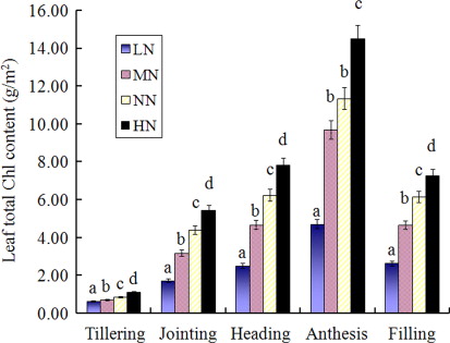
At different growth stages, the order of wheat LTCC under different N treatments was: high nitrogen (HN) > normal nitrogen (NN) > medium nitrogen (MN) > low nitrogen (LN) (Fig. 1). Due to there being no significant differences between the three cultivars [according to analysis of variance (ANOVA) analysis], the average LTCC values were used for the different treatments. ANOVA results showed that LTCC exhibited significant differences under different N levels at tillering, jointing, heading, anthesis and filling stages (Fig. 1). This was so with the exception of the anthesis stage, which showed no significant differences at NN and MN levels. With growth stage development, LTCC gradually increased under different N levels. The LTCC significant differences were the highest at the heading stage and decreased apparently at the filling stage. These results indicated that wheat leaf fading led to a sharp LTCC decrease at the later stage of plant growth. The significant differences order was: heading, filling, jointing, tillering and anthesis. The results suggested that LTCC increased as growth stages progressed; however, each increment of increase was different. The incremental order was: MN > NN > HN > LN (Fig. 1).

Figure 1 The change trends of leaf total chlorophyll content (LTCC) under different nitrogen treatments (the average value of three wheat cultivars). The LTCC for tillering, jointing, heading, anthesis and filling of wheat subjected to under low (LN, 0 kg N/ha), medium (MN, 105 kg N/ha), normal (NN, 225 kg N/ha) and high (HN, 345 kg N/ha) levels of N application over five cropping seasons (2009 and 2010). Data are average values across 2 years with +one standard error (vertical bars). Analysis of variance (ANOVA) results for tillering: N, P<0.007, wheat cultivars (C), P<0.123; jointing: N, P<0.004, C, P<0.078; heading: N, P<0.0001 C, P<0.102; anthesis: N, P<0.002 C, P<0.112; filling: N, P<0.007 C, P<0.09.

Reflectance changes in the different LTCC levels

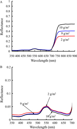
We selected LTCC at 2, 9 and 10 g/m² at N3 treatment, to study spectral reflectance changes with different LTCC levels. Results showed that the different LTCC levels had significant differences at the NIR ranges (Fig. 2a), the green range (around 550 nm), and the range of the red edge (near 700 nm) (Fig. 2b). The highest, lowest and median reflectance were the LTCC of 10, 2 and 9 g/m² at the NIR ranges, and the LTCC of 2, 10 and 9 g/m² at green range, respectively. The results indicated that the higher NIR reflectance value did not correspond to the higher reflectance in the green (around 550 nm) and that in the red edge range (near 700 nm). Thus, reflectance was affected by LTCC changes. ANOVA results showed that LTCC exhibited significant differences under different N levels (Figs. 2a and b).

Figure 2 Relationship between reflectance and leaf total chlorophyll content (LTCC) at N3 treatment: (a) the different LTCC reflectance at near 700 nm, (b) the different LTCC reflectance around 550 nm. The LTCC (2, 9 and 10 g/m²) for A and B, analysis of variance (ANOVA) results for A, P<0.002; B, P<0.021.

Spectral characteristics of leaves and their relationships with LTCC

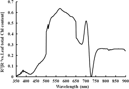
We studied the reciprocal reflectance behaviour of R ² to find out whether the reciprocal reflectance was sensitive to LTCC. The 36 data points were selected from all growth stages of wheat. The data show the correlation relationship between spectral reflectance and LTCC for the different nitrogen treatments (Fig. 3). LTCC and spectral reflectance were slightly correlated at 350–450 nm, and the lowest value of the coefficient of determination (R ²) was 0.01 at 350 nm. Spectral reflectance exhibited a significant correlation with LTCC and the coefficient of determination (R ²) was higher than 0.40 from 500 to 650 nm. The highest R ² value was 0.67 at 572 nm. This value reduced sharply at around 652 nm and the lowest R ² value was 0.31 at 682 nm. Following these relative high and low values, from 650 to 750 nm the highest value was 0.52 at 704 nm, and the lowest value was 0.01 at 730 nm. The R ² then changed slightly, and was subsequently maintained at around 0.26 from 750 to 900 nm.

Figure 3 The coefficient of determination (R ²) between leaf total chlorophyll content (LTCC) and spectral reflectance in wheat.

Spectral parameters selection and stepwise regression methods

Twenty spectral parameters were selected according to the significant relationships between spectral parameters and LTCC; further analysis is required to establish an estimation model (Table 1). Linear and non-linear regression analysis was done using the selected spectral parameters as independent variables (Table 2).

Table 1 Summary of selected vegetation indices, wavebands and citations for chlorophyll.

Index	Wavebands	Reference
	R 550	Carter (1994)
	log(1/R 737)	Yoder & Pettigrew-Crosby (1995)
SIPI	(R 800–R 445)/(R 800–R 680)	Penuelas et al. (1995)
Ratcart	R 695/R 760	Carter et al. (1996)
PSSRa	R 800/R 680	Blackburn (1998)
PSSRb	R 800/R 635	Blackburn (1998)
PSNDa	(R 800–R 675)/(R 800+R 675)	Blackburn (1998)
PSNDb	(R 800–R 650)/(R 800+R 650)	Blackburn (1998)
PSSRchla	R 810/R 676	Blackburn (1999)
PSRI	(R 680–R 500)/R 750	Merzlyak et al. (1999)
SR705	R 750/R 705	Sims and Gamon (2002)
ND705	(R 750–R 705)/(R 750+R 705)	Sims and Gamon (2002)
mND705	(R 750–R 445)/(R 700–R 445)	Sims and Gamon (2002)
mSR705	(R 750–R 705)/(R 750+R 705–2R 445)	Sims and Gamon (2002)
Readone	R 415/R 695	Read et al. (2002)
RGRcan	(R 612+R 660)/(R 510+R 560)	Steddom et al. (2003)
NDVIcanste	(R 760–R 708)/(R 760+R 708)	Steddom et al. (2003)
Red edge Model	(R 800/R 700)–1	Gitelson et al. (2005)
Green Model	(R 800/R 550)–1	Gitelson et al. (2005)
EVI2	EVI2 = 2.5×(R 800–ρ660)/(1 + ρ800+2.4×ρ660)	Jiang et al. (2008)

R _i denotes reflectance at band i (nanometer).

Table 2 The correlation coefficient (r) between leaf total chlorophyll content (LTCC) and the spectral indices (n=90).

Vegetation indices	Correlation coefficient (r)	RMSE (g/m^2) (n=60)
R550	0.8013**	2.43
log(1/R 737)	0.6234**	4.53
SIPI	0.7545**	3.43
Ratcart	0.8912**	1.32
PSSRa	0.8875**	1.63
PSSRb	0.8914**	1.54
PSNDa	0.8467**	1.98
PSNDb	0.8322**	2.04
PSSRchla	0.8563**	1.92
PSRI	−0.8042**	2.46
SR705	0.8950**	1.28
ND705	0.8925**	1.38
mND705	0.8554**	1.89
mSR705	0.8746**	1.72
Readone	0.4992**	5.24
RGRcan	0.8580**	1.92
NDVIcanste	0.8925**	0.93
Red edge Model	0.8945**	0.72
Green Model	0.9023**	0.84
EVI2	0.8743**	1.68

n=number of pairs of data. **Model significant at the 0.01 level of probability.

We subsequently studied correlations between spectral parameters and LTCC under different levels of N levels (Table 2). The results indicated that the relationships between LTCC and all spectral parameters arrived at significant levels. PSRI was significantly negatively correlated with LTCC, and the correlation coefficient (r) was −0.8042. The remaining parameters were positively correlated with LTCC and the Green Model had the highest correlation coefficient value of 0.9023. The results showed that all the spectral parameters were significantly correlated with LTCC. The following parameters were significantly positively correlated to LTCC: Ratcart, PSSRb, NDVIcanste, Red edge Model, SR705 and Green Model; the respective r values were 0.8912, 0.8914, 0.8925, 0.8945, 0.8950 and 0.9023. This suggested that Ratcart, PSSRb, NDVIcanste, Red edge Model, SR705 and Green Model could be used to estimate total Chl content for wheat. Ninety pairs of data were used to establish the regression model (calibration model n=90) from 2009. Results showed that regression models for these indices were feasible for predicting LTCC (Fig. 4). To validate regression models, we used validation data (n=60) from 2010.

Figure 4 Quantitative relationships of the leaf total chlorophyll content (LTCC) to Green Model A, SR705; B, Red edge Model; C, Ratcart; D, NDVIcanste; E, and PSSRb; F, respectively, in winter wheat (n=90). †x represents spectral indices; y represents LTCC.

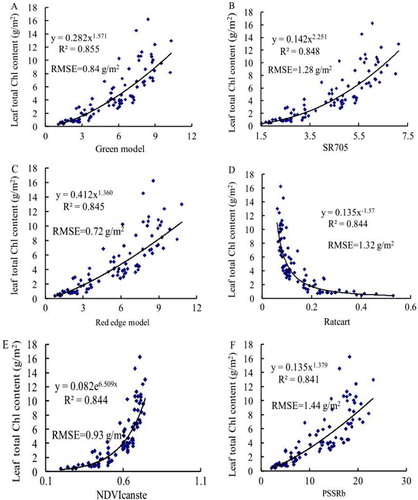
The Green Model, SR705, Red edge Model, Ratcart and PSSRb were fitted to power regression models (Figs. 4a–d and f), but the NDVIcanste was fitted to an exponential regression model (Fig. 4e). The highest and lowest correlation coefficients were those of Green Model and PSSRb, with determination coefficient (R ²) values of 0.8553 and 0.8412 in all simulation models (Figs. 4a and f). The order of R ² values was: Green Model, SR705, Red edge Model, Ratcart, NDVIcanste and PSSRb. The order of RMSE values was: Red edge Model, Green Model, NDVIcanste, SR705, Ratcart and PSSRb. The indices with the highest and lowest RMSE values were Red edge Model and PSSRb, with values of 0.72 and 1.44 g/m², respectively (Fig. 4).

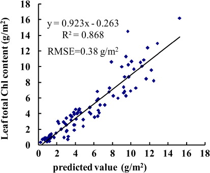
To establish a new index regression model, using SRM, we combined Green Model, SR705, Red edge Model, Ratcart, NDVIcanste and PSSRb. First, we added in each of the six vegetation indices and, accounting for weight to predict LTCC, added the best remaining variable. Second, all variables currently in the regression were checked to see if any could be removed, using the greater than 10% significance criterion test. The process continued until no more variables could be added or removed. Finally, we obtained the new index: 3.575Red edge Model–1.118PSSRb; the R ² for estimation of LTCC was 0.87 (Fig. 5). To validate the model accuracy, we compared predicted values with actual values by using data from 2010, and the results showed that the RMSE was 0.38 g/m² (Fig. 5). The results demonstrated that the 3.575Red edge Model–1.118PSSRb index could be used to improve LTCC prediction accuracy.

Figure 5 Quantitative relationships of the leaf total chlorophyll content (LTCC) to 3.575Red edge model–1.118PSSRb in wheat (n=90).

Partial least squares regression

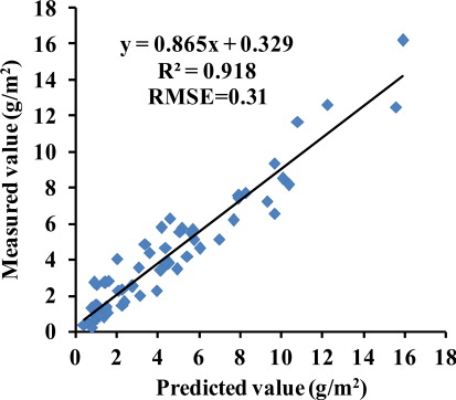
To improve the estimation accuracy of LTCC, using PLS, we combined Green Model, SR705, Red edge Model, Ratcart, NDVIcanste and PSSRb. The final regression model for the estimation of LTCC yielded a R ² value of 0.92. To validate the model accuracy, we compared predicted values with actual values and the results showed that the RMSE was 0.31 g/m² (Fig. 6). The results demonstrated that the PLS could also be used to improve LTCC prediction accuracy.

Figure 6 Relationships between predicted leaf total chlorophyll content (LTCC) and actual LTCC by using partial least squares (PLS).

Discussion

The objective of our work was to evaluate the use of hyperspectral parameters as a non-destructive technology to assess LTCC in wheat. In this work, we used a sensor with a spectral range from 350 to 1000 nm. Wheat LTCC was lowest in the tillering stage, and it then increased as the plant developed into the anthesis stage. This resulted from the sharp dry matter accumulation with the progression of plant development. Dry matter accumulation in the field of view of the spectrometer could obviously also affect the spectral signature—it is always slightly doubtful whether indices created at canopy level portray evolution in chl or change in biomass per se. For this reason, leaf spectral measurements would also have been desired. The different LTCC had significant differences at the green range (around 550 nm) and the red edge (near 700 nm) (Fig. 2), for which R ² was 0.67 and 0.52 at 572 and 704 nm, respectively (Fig. 3). These results were similar to those obtained by Carter (1994) and Sims & Gamon (2002). Twenty spectral parameters were used to predict LTCC, and all the spectral parameters had a significant correlation with LTCC. LTCC correlations were highly significant for Green Model, SR705, Red edge Model, Ratcart, NDVIcanste and PSSRb (Fig. 4). These results suggested that these six spectral indices could be used to estimate LTCC. The results were in agreement with those of a recent study based on simulated data in the literature (Carter et al. 1996; Blackburn 1998; Sims & Gamon 2002; Steddom et al. 2003; Gitelson et al. 2005). However, these indices were non-sensitive to LTCC at lower levels, and saturation could occur with these indices at higher LTCC levels (Fig. 4).

Using SRM, we obtained a new index: 3.575Red edge Model–1.118PSSRb (Fig. 5). It was better able to predict LTCC than the six indices alone were. The RMSE of 3.575Red edge Model–1.118PSSRb was lower than that of the Red edge Model, which was the best LTCC estimation model of the above vegetation indices (Figs. 4 and 5). Haboudane et al. (2002) and Zarco-Tejada et al. (2004) indicated that combined indices improved LTCC estimation when compared with single indices. This was because the combined indices were not only more sensitive to LTCC, but were also less negatively influenced by variations in LAI and soil background reflectance (Eitel et al. 2008). Across 2 years and growth stages, 3.575Red edge Model–1.118PSSRb could explain 87% of wheat LTCC variability, which was more than any other vegetation index could explain (Fig. 5). This suggested that the combination index could be used to improve the prediction accuracy of LTCC. It is composed of wavelengths at 800, 700 and 635 nm. It showed that 635 and 700 nm had a highly significant correlation with LTCC (Fig. 3), and 700 nm was deeply absorbed by Chl at the near red edge. The 800 nm was at NIR ranges and was mainly affected by canopy layers; the prediction accuracy of LTCC decreased as canopy layers increased. The 3.575Red edge Model–1.118PSSRb could also decrease the effect of canopy layers. This explained why the prediction accuracy of 3.575Red edge Model–1.118PSSRb of LTCC was higher when compared with any of the six indices alone. The two involved indices contain some distinct and independent information that contribute to improvement of LTCC estimation accuracy. The results showed that PLS was better than SRM, as it considered the effects of more than one spectral index. It may be provide a regression model where the entire spectral information is taken—in a weighted form—into account; it seems therefore much better adapted to deal with potentially confounding factors than SRM. Some authors indicated that PLS was better than SRM (Atzberger et al. 2010; Song et al. 2011); our results were consistent with these results.

The results indicated that different spectral parameters could be collected at all wheat growth stages. Furthermore, these spectral parameters could be combined, via SRM or PLS, to improve the estimation accuracy of LTCC. This method led to the innovative idea that a more accurate prediction of LTCC could be attained by combining different spectral parameters. Also, the refinement of spectral parameter inclusion aimed to reduce other affected factors. Future studies should consider a wide range of canopy conditions. Furthermore, research should aim to build a more extensive database containing data from different locations and years; such data is required to strengthen the relationships between the VIs and LTCC.

Conclusion

Building upon previous studies, LTCC was predicted using vegetation indices and SRM, and the main results and conclusions follow. The wheat LTCC order was: high nitrogen (HN) > normal nitrogen (NN) > medium nitrogen (MN) > low nitrogen (LN) across all growth stages. LTCC had significant differences under different N stress levels at tillering, jointing, heading, anthesis and filling stages, with the exception that the anthesis had no significant differences at the NN and MN levels. Reflectance changes in the different LTCC indicated that the higher LTCC values corresponded to higher reflectance at the NIR ranges. The higher NIR reflectance value did not correspond to the higher reflectance in the green (around 550 nm) and in the range of the red edge (near 700 nm). This suggested that reflectance was affected by changes in LTCC. Spectral characteristics of leaves and their relations with LTCC proved that LTCC and spectral reflectance were slightly correlated at 350–450 nm, but had a significant correlation from 500 to 650 nm (R ² was higher than 0.4). The highest value was 0.67 at 572 nm. We combined Green Model, SR705, Red edge Model, Ratcart, NDVIcanste and PSSRb by SRM or PLS, SRM obtained a new index: 3.575Red edge Model–1.118 PSSRb. The R ² was 0.87 and the RMSE was 0.38 g/m². PLS gained the R ² and RMSE of regression model were 0.92 and 0.31 g/m².

Acknowledgments

The study is supported by the National Natural Science Foundation of China (Grant No. 31071371 and No. 41161068), and the Key Projects in the National Science & Technology Pillar Program during the Eleventh Five-Year Plan Period (Grant No. 2012BAH27B04). The authors would also like to thank the staff at the Agricultural Remote Sensing Center, Key Laboratory of Oasis Ecology Agriculture of Xinjiang Construction Crops.

References

- Atzberger C, Guérif M, Baret F, Werner W 2010. Comparative analysis of three chemometric techniques for the spectroradiometric assessment of canopy chlorophyll content in winter wheat. Computers and Electronics in Agriculture 73: 165–173. 10.1016/j.compag.2010.05.006
- Blackburn GA 1998. Quantifying chlorophylls and carotenoids at leaf and canopy scales: an evaluation of some hyper-spectral approaches. Remote Sensing of Environment 66: 273–285. 10.1016/S0034-4257(98)00059-5
- Blackburn GA 1999. Relationships between spectral reflectance and pigment concentrations in stacks of deciduous broadleaves. Remote Sensing of Environment 70: 224–237. 10.1016/S0034-4257(99)00048-6
- Buschmann C, Nagel E 1993. In vivo spectroscopy and internal optics of leaves as basis for remote sensing of vegetation. International Journal of Remote Sensing 14: 711–722. 10.1080/01431169308904370
- Carter GA 1994. Ratios of leaf reflectances in narrow wavebands as indicators of plant stress. International Journal of Remote Sensing 15: 697–703. 10.1080/01431169408954109
- Carter GA, Cibula WG, Miller RL 1996. Narrow-band reflectance imagery compared with thermal imagery for early detection of plant stress. Journal of Plant Physiology 148: 515–522. 10.1016/S0176-1617(96)80070-8
- Carter GA, Knapp AK 2001. Leaf optical properties in higher plants: linking spectral characteristics to stress and chlorophyll concentration. American Journal of Botany 84: 677–684. 10.2307/2657068
- Chappelle EW, Kim MS, McMurtreyIII JE 1992. Ratio analysis of reflectance spectra (RARS): an algorithm for the remote estimation of the concentrations of chlorophyll a, chlorophyll b, and carotenoids in soybean leaves. Remote Sensing of Environment 39: 239–247. 10.1016/0034-4257(92)90089-3
- Datt B 1998. Remote sensing of chlorophyll a, chlorophyll b, chlorophyll a + b, and total carotenoid content in eucalyptus leaves. Remote Sensing of Environment 66: 111–121. 10.1016/S0034-4257(98)00046-7
- Eitel JUH, Long DS, Gessler PE, Hunt ER 2008. Combined spectral index to improve ground-based estimates of nitrogen status in dryland wheat. Agronomy Journal 100: 1694–1702. 10.2134/agronj2007.0362
- Gamon JA, Surfus JS 1999. Assessing leaf pigment content and activity with a reflectometer. New Phytologist 143: 105–11710.1046/j.1469-8137.1999.00424.x.
- Gitelson AA, Merzlyak MN 1994a. Quantitative estimation of chlorophyll a using reflectance spectra: experiments with autumn chestnut and maple leaves. Journal of Photochemistry and Photobiology B 22: 247–252. 10.1016/1011-1344(93)06963-4
- Gitelson AA, Merzlyak MN 1994b. Spectral reflectance changes associated with autumn senescence of Aesculus hippocastanum and Acer platanoides leaves. Spectral features and relation to chlorophyll estimation. Journal of Plant Physiology 143: 286–292. 10.1016/S0176-1617(11)81633-0
- Gitelson AA, Merzlyak MN 1996. Signature analysis of leaf reflectance spectra: algorithm development for remote sensing of chlorophyll. Journal of Plant Physiology 148: 494–500. 10.1016/S0176-1617(96)80284-7
- Gitelson AA, Merzlyak MN 1997. Remote estimation of chlorophyll content in higher plant leaves. International Journal of Remote Sensing 18: 291–298. 10.1080/014311697217558
- Gitelson AA, Merzlyak MN, Chivkunova OB 2001. Optical properties and non-destructive estimation of anthocyanin content in plant leaves. Journal of Photochemistry and Photobiology 74: 38–45. 10.1562/0031-8655(2001)074<0038:OPANEO>2.0.CO;2
- Gitelson AA, Zur Y, Chivkunova OB, Merzlyak MN 2002. Assessing carotenoid content in plant leaves with reflectance spectroscopy. Journal of Photochemistry and Photobiology 75: 272–281. 10.1562/0031-8655(2002)075<0272:ACCIPL>2.0.CO;2
- Gitelson AA, Vina A, Ciganda V, Rundquist DC, Arkebauer TJ 2005. Remote estimation of canopy chlorophyll content in crops. Geophysical Research Letters 32: L08403. 10.1029/2005GL022688
- Gitelson AA, Vina A, Verma SB, Rundquist DC, Arkebauer TJ, Keydan G, Leavitt B, Ciganda V, Burba GG, Suyker AE 2006. Relationship between gross primary production and chlorophyll content in crops: implications for the synoptic monitoring of vegetation productivity. Geophysical Research Letters 111: D08S11. 10.1029/2006JD006017
- Haboudane D, Miller JR, Tremblay N, Zarco-Tejadad PJ, Dextrazec L 2002. Integrated narrow-band vegetation indices for prediction of crop chlorophyll content for application to precision agriculture. Remote Sensing of Environment 81: 416–426. 10.1016/S0034-4257(02)00018-4
- Jiang Z, Huete AR, Didan K, Miura T 2008. Development of a two-band enhanced vegetation index without a blue band. Remote Sensing of Environment 112: 3833–3845. 10.1016/j.rse.2008.06.006
- Le Maire G, Francois C, Dufrene E 2004. Towards universal broad leaf chlorophyll indices using PROSPECT simulated database and hyperspectral reflectance measurements. Remote Sensing of Environment 89: 1–28. 10.1016/j.rse.2003.09.004
- Lichtenthaler HK, Gitelson AA, Lang M 1996. Non-destructive determination of chlorophyll content of leaves of a green and an aurea mutant of tobacco by reflectance measurements. Journal of Plant Physiology 148: 483–493. 10.1016/S0176-1617(96)80283-5
- Lieth H, Whittaker RH 1975. Primary production of the biosphere. New York, Springer.
- Li M, Han D, Wang X 2006. In: Li M ed. Spectrum analysis technique and applications. Beijing, Science Press. Pp. 176–183 ( in Chinese).
- Markwell J, Osterman JC, Mitchell JL 1995. Calibration of the Minolta SPAD-502 leaf chlorophyll meter. Photosynthesis Research 46: 467–472. 10.1007/BF00032301
- McKinney G 1941. Absorption of light by chlorophyll solutions. Journal of Biological Chemistry 140: 315–322.
- Merzlyak MN, Gitelson AA, Chivkunova OB, Rakitin VY 1999. Non-destructive optical detection of pigment changes during leaf senescence and fruit ripening. Physiologia Plantarum 106: 135–141. 10.1034/j.1399-3054.1999.106119.x
- Penuelas J, Baret F, Filella I 1995. Semiempirical indices to assess carotenoids chlorophyll-a ratio from leaf spectral reflectance. Photosynthetica 31: 221–230.
- Peng SB, Huang JL, Zhong XH, Yang JC, Wang GH, Zou YB, Zhang FS, Zhu QS, Buresh R, Witt C 2002. Research strategy in improving fertilizer nitrogen use efficiency of irrigated rice in China. Scientia Agricultura Sinica 35: 1095–1103 ( in Chinese).
- Peng Y, Gitelson AA, Keydan G, Rundquist DC, Moses W 2011. Remote estimation of gross primary production in maize and support for a new paradigm based on total crop chlorophyll content. Remote Sensing of Environment 115: 978–989. 10.1016/j.rse.2010.12.001
- Read JJ, Tarpley L, McKinion JM, Reddy KR 2002. Narrow-waveband reflectance ratios for remote estimation of nitrogen status in cotton. Journal of Environmental Quality 31: 1442–1452. 10.2134/jeq2002.1442
- Richardson AD, Duigan SP, Berlyn GP 2002. An evaluation of noninvasive methods to estimate foliar chlorophyll content. New Phytologist 153: 185–194. 10.1046/j.0028-646X.2001.00289.x
- Sims DA, Gamon JA 2002. Relationship between leaf pigment content and spectral reflectance across a wide range species, leaf structures and development stages. Remote Sensing of Environment 81: 337–354. 10.1016/S0034-4257(02)00010-X
- Song KS, Lu DM, Li L, Li S, Wang ZM, Du J 2011. Remote sensing of chlorophyll-a concentration for drinking water source using genetic algorithms (GA)–partial least square (PLS) modeling. Ecological Informatics 10: 25–36. 10.1016/j.ecoinf.2011.08.006
- Steddom K, Heidel G, Jones D, Rush CM 2003. Remote detection of rhizomania in sugar beets. Phytopathology 93: 720–726. 10.1094/PHYTO.2003.93.6.720
- Wood CW, Tracy PW, Reeves DW, Edmisten KL 1992. Determination of cotton nitrogen status with a hand-held chlorophyll meter. Journal of Plant Nutrition 15: 1435–1448. 10.1080/01904169209364409
- Yoder BJ, Pettigrew-Crosby RE 1995. Predicting nitrogen and chlorophyll content and concentrations from reflectance spectra (400–2500 nm) at leaf and canopy scales. Remote Sensing of Environment 53: 199–211. 10.1016/0034-4257(95)00135-N
- Zarco-Tejada PJ, Miller JR, Morales A, Berjon A, Aguera J 2004. Hyperspectral indices and model simulation for chlorophyll estimation in open-canopy crops. Remote Sensing of Environment 90: 463–476. 10.1016/j.rse.2004.01.017
- Zhu Z, Wen Q 1992. Soil nitrogen in China. Nanjing, Jiangsu Science and Technology Press. Pp. 213–249 ( in Chinese).