A preliminary model of sweet corn growth and yield

ABSTRACT

A model is developed to assist forecasting and interpretation of crop performance of sweet corn (Zea mays L.) under optimal nutrient supply. Leaf area growth is calculated on the main stem and tillers separately using a discrete logistic equation that includes adjustments for soil water deficit (D). Leaf senescence depends on age and D. The conversion efficiency for intercepted radiation to biomass also varies with D. Ear dry mass is computed assuming harvest index varies linearly with thermal time. The model was fitted using a dataset for crop responses to D, tested against data for responses to sowing date, refitted using both datasets, and retested against measurements of growth across a wide range of plant populations. Model performance was excellent for leaf area and biomass. It was less good for ear dry mass, although regression of observed on simulated values gave slopes not significantly different from 1. Priorities for further development are discussed.

KEYWORDS:

• Zea mays L
• crop model
• leaf area
• plant population
• water stress

View correction statement:

Corrigendum

Introduction

Worldwide, sweet corn (Zea mays L.) is an important vegetable crop. Annual production in New Zealand is about 91,000 tonnes, worth about NZ$59 million (Aitken & Hewett 2016). Despite this importance, there is a lack of published and widely accepted models of both growth and development that can be used for forecasting or interpreting sweet corn responses to environmental conditions or management inputs. This contrasts with the situation for maize where there are many such models (Stapper & Arkin 1980; Sinclair & Muchow 1995; Wilson et al. 1995; Reid et al. 1999; Jones et al. 2003; Jamieson et al. 2008; Brown et al. 2015).

Lizaso et al. (2007) developed the only model for growth and development of sweet corn published so far. For this, they adapted the earlier CERES-Maize model (Jones et al. 2003) by changing the description of ear and kernel growth and development. In practice, management and genetic factors differ between the two crops in ways that are not confined to ear and kernel growth. A comparison of results obtained at the same site by Stone et al. (2001) and Jamieson et al. (1995) indicates that sweet corn yield is roughly twice as sensitive to water deficits as maize. Aslam (2005) observed significant differences between sweet corn and maize in root growth and response to phosphorus (P) supply. Rogers et al. (1999) examined leaf area growth and senescence from several experiments, and found important differences between sweet corn and maize; in particular, sweet corn leaf area senesced considerably more slowly. Their results suggest that even if the same model framework is used for both crops, different parameter values for leaf area growth and duration are highly desirable. Lizaso et al. (2007) did not report the performance of their sweet corn model for leaf area production. However, the underlying maize model assumes specific leaf area (m² g⁻¹) varies only with total plant leaf area. In sweet corn, specific leaf area may vary substantially also with soil water deficit (Stone et al. 2001), and Yang et al. (2009) suggested improvements to the model’s description of leaf area production even for maize.

The objective of this paper is to report the development and testing of a new model for sweet corn growth that has potential to be adapted by both industry and the science community for forecasting and interpreting crop growth and yield. A consistent theme through the development was to keep the model’s requirements for input variables and fitted parameter values as modest as possible while keeping the description of key processes sufficiently mechanistic that the final model has considerable portability between environments. Accordingly, the model simulates leaf area dynamics independently of biomass production (Tardieu et al. 1999), total dry matter production as a simple function of intercepted radiation (Charles-Edwards 1982), harvest index as a linear function of thermal time (Muchow 1990). It is narrower in scope than the model of Lizaso et al. (2007); at this stage, it does not consider ear quality, dry matter partitioning into leaves and stems, or nutrient effects. There is strong evidence that yield is markedly affected by water stress (Stone et al. 2001), planting date (Rogers et al. 2000), and population density (Stone et al. 1998), and excellent datasets are available for developing and testing a sweet corn model that includes such effects. The prime focus here is to consider the model’s ability to simulate leaf area dynamics and yield when such effects are operating but nutrient supply is not limiting.

Model description

For brevity, the names, symbols, values, and units of the variables and parameters are defined in Tables 1 and 2. The subscripts used for the symbols are important; n denotes a day number after sowing, ø denotes under potential (unstressed) conditions, and p denotes a value for the whole plant. The model simulates crop growth using a daily time step. At this stage, it assumes the effects of photoperiod on crop development are minor, consistent with the conclusions of Brooking and McPherson (1989) and Olsen et al. (1993).

Table 1. List of variables used in the model of sweet corn growth and yield.

Symbol	Definition	Units	Notes
A	Soil available water capacity	mm	228 mm for Dataset 1, 180 mm for Datasets 2 and 3
D	Soil water deficit—the difference in soil water content from field capacity	mm
D*	Scaled soil water deficit
EØp	Potential transpiration	mm	Priestley and Taylor (1972), Ritchie (1972)
Etransp	Transpiration	mm
Esoil	Soil surface evaporation	mm
G	Green leaf area index
H	Harvest index
I	Irrigation applied	mm
L	Leaf area index		Separate values calculated for main stem and tillers
Lmax	Maximum possible value of L		Separate values calculated for main stem and tillers
Mear	Dry mass of ears	g m^−2
Mp	Dry mass of crop (total above ground)	g m^−2
n	Days after sowing	d
P	Rainfall received	mm
p	Plant population density	m^−2
Q	Daily incident radiation	MJ m^−2
s	Cumulative leaf area index susceptible to senescence
S	Cumulative senescent leaf area index
t	Thermal time from sowing	°C d
Tavg	Daily average air temperature	°C
Wg	Stress factor for calculation of leaf area growth
Wr	Stress factor for calculation of σ
Ws	Stress factor for calculation of leaf area senescence
Σ	Radiation conversion efficiency	g MJ^−1

Table 2. List of parameters used in the model of sweet corn growth and yield.

Symbol	Definition	Units	Value	Source and notes
cg	Empirical constant for calculation of Wg		1.60	Fitted
cr	Empirical constant for calculation of Wr		50	Fitted
cs	Empirical constant for calculation of Ws		1.66	Fitted
D*crit.transp	Critical value of D* for transpiration		0.5	Johns and Smith (1975), Baird et al. (1986)
dg	Empirical constant for calculation of Wg		0.260	Fitted
dr	Empirical constant for calculation of Wr		0.594	Fitted
ds	Empirical constant for calculation of Ws		1.79	Fitted
h	Rate of increase in H with t	(°C d)^−1	6.33 × 10^−4	Fitted
Hsilk	Harvest index at the time of silking		0.140	Fitted
k	Canopy light extinction coefficient		0.4	Ritchie (1972)
linit	Leaf area per plant on day of emergence	m^2	9.00 × 10^−4	Fitted
lØ.mainstem	Potential leaf area per plant on main stem	m^2	0.530	Fitted
lØ.tiller1	Potential leaf area per plant on tiller 1	m^2	0.300	Fitted
lØ.tiller2	Potential leaf area per plant on tiller 2	m^2	0.100	Fitted
Nmax.mainstem	Max. number of main stem leaves		17	Observed in fitting dataset
Nmax.tiller1	Max. number of leaves on tiller 1		14	Observed in fitting dataset
Nmax.tiller2	Max. number of leaves on tiller 2		8	Observed in fitting dataset
Tb	Base temperature for thermal time calculation	°C	5	Stone (personal communication 2016)
temer	Thermal time from sowing to emergence	°C d	86.6	Observed in fitting dataset
tmat	Thermal time from sowing to harvestable maturity	°C d	1408	Observed in fitting dataset
ts	Life expectancy of leaf area	°C d	441	Fitted
tsilk	Thermal time from sowing to silking	°C d	807	Observed in fitting dataset
α	Constant for daily growth in L	(°C d)^−1	0.0130	Fitted
ηtiller1	Mainstem node number from which tiller 1 emerges		4	Observed in fitting dataset
ηtiller2	Mainstem node number from which tiller 2 emerges		6	Observed in fitting dataset
σmin	Lower limit of σ under stress	g m^−2	0.949	Fitted
σØ	Radiation conversion efficiency for an unstressed crop	g m^−2	1.47	Fitted
Ω	t interval between complete expansion of successive leaves	°C d	46.5	Observed in fitting dataset

Thermal time (t, °C d) is calculated from daily average screen air temperatures (T_avg) and a base temperature T_b:(1) Crop emergence occurs when t first exceeds a constant t_emer. Silking occurs when t first exceeds t_silk, and the crop is deemed to be at harvestable maturity when t ≥ t_mature. Physiologically, it is probably best to calculate t from measurements of T for the apical meristem, at least until ears emerge. Practically, that is problematic. During germination, emergence and until 5 or 6 true leaves are emerged t may be approximated from soil temperatures (Stone et al. 1998, 1999) and by air temperatures thereafter. However, the soil depths or above ground heights at which that temperature is recorded or estimated will vary with time, and appropriate daily mean values are not readily available from most standard meteorological sites. Here we have assumed that T_avg is adequately approximated from air temperatures at a standard screen height (1.3 m). Future refinements of the model may include soil and air temperatures. Brooking and McPherson (1989) examined crop records for the areas around Feilding, Gisborne, and Hastings in the North Island of New Zealand and proposed that T_b was 6°C when T is calculated from air temperature. Stone (personal communication 2016) estimated T_b to be 5°C, based on an analysis of crop records from around Tolaga Bay, Gisborne, Wairoa, and Hastings in New Zealand and from around Griffith and Hillstone in New South Wales, Australia. Caution must be exercised in directly comparing those values or attempting physiological interpretations of them. Neither was based on direct observation of crop development under controlled temperature conditions. Both are simply values associated with the best statistical fits of the crop development models and datasets those researchers used, and also their particular ways of estimating T_avg. Here we follow Stone and take T_b = 5°C with T_avg calculated as the average of the daily maximum and minimum air temperatures. Those choices can be modified by subsequent users of this model but any optimised model parameters dependent on those assumptions must also be adjusted accordingly.

We assume the crop may produce two potentially viable tillers, which emerge at nodes η₁ and η₂, respectively. (Two potential tillers were chosen on the basis of the datasets available for model development and testing, but the number is readily changed.) The number of fully emerged leaves (N) on the main stem and tillers varies with t:(2a) (2b) (2c) where N_max is the maximum number of leaves (treated as a constant for the hybrid), and Ω is the interval in t between complete expansion of successive leaves. The progression in N_tiller1 and N_tiller2 with t is stopped abruptly by stress.

Total biomass production is assumed directly proportional to light intercepted by the canopy, which is simulated using a Beer–Lambert analogue (Lemeur & Blad 1974; Monteith 1977; Charles-Edwards 1982; Stone et al. 2001):(3) where Q is the daily incident radiation, σ is the radiation conversion efficiency, G_n is the green leaf area index, and k is the canopy’s light extinction coefficient. Stone et al. (2001) found that the seasonal value of σ decreased as the maximum potential soil water deficit increased. Here we need daily values of σ and we assume:(4) where σ_ø is the unstressed radiation use efficiency, σ_min is a lower limit of σ, and W_r is a stress factor (see below). This is a necessary simplification in the absence of fuller information on short-term variations in σ.

Harvest index (H, the fraction of crop dry matter allocated to ears) increases linearly with thermal time after silking (Muchow 1990):(5) where H_silk and h are empirical constants. The dry ear yield is calculated from:(6)

Total leaf area index (L) is the sum of L for the main stem and tillers; for each of these the daily growth increment in L is described by:(7a) (7b) (7c) where L_max is the maximum leaf area index that the plant can achieve on the main stem or tiller, l_init is the initial leaf area on the day of emergence (m² plant⁻¹), ρ is the plant population density (plants m⁻²), W is a stress factor (see below), and α is a constant with units of (°C d)⁻¹. Equation (7c) is a form of discrete logistic equation. Note that fitted values of l_init may be larger than leaf areas measured immediately after the first leaf appears on the main stem or tiller. Leaf area growth in the first few days is influenced by plant reserves as well as daily dry matter growth. Furthermore, for simplicity here, we use the same value of l_init for the first leaf on the main stem and on the tillers. Therefore, l_init should be interpreted as something of an average over that period as well as an average over the main stem and tillers.

For the main stem and each tiller, L_max is calculated separately. In the absence of stress, it is equivalent to (l_Ø ρ), where l_Ø is the potential maximum leaf area on the main stem or tiller (m² plant⁻¹). Models of indeterminate crops may treat L_max as a constant (Reid & English 2000), but that is not the case here. If on any given day leaf area expansion has been slowed by stress, then the model permanently reduces the future L_max by the amount of growth lost on that day. On the basis of experience with the datasets used here, for tillers both leaf expansion and the progression in leaf appearance are abruptly and permanently stopped by stress.

The green leaf area index (G) increases in the same way as L, but the cumulative area of senescent leaf material (S) has to be subtracted:(8) To calculate S_n first we identify s_n, the amount of leaf area that is susceptible to senescence because it is older than t_s degree days but has not already senesced:(9) where ns is the latest day number that meets the criterion (t_n–t_ns≥ t_s). The fraction of susceptible leaf area that does senesce on a given day depends on a stress factor (W_s):(10) The term (1–W_sn)² represents the fraction of s_n that senesces on day n.

Stress factors

For now we assume that the stress factors for leaf area growth (W_g), radiation use efficiency (W_r), and leaf area senescence (W_s) are due solely to water stress, and vary smoothly with the soil water deficit D (the difference between profile water content in mm water at field capacity and that on day n). The daily progression in D is calculated as:(11) (See Table 1 for definitions.) To assist portability of the model between environments, rather than use D directly to calculate water stress, we use the scaled soil water deficit D_*, defined as D divided by the soil’s available water capacity (A). D_* is confined to values between 0 and 1. In applying Equation (11), drainage is assumed to be zero, which is a safe assumption for the datasets analysed in this paper. Daily incoming radiation is partitioned between potential transpiration (E_Øp) and E_soil according to the model of Ritchie (1972) with the calculation of E_soil simplified according to Reid (1990). E_transp is calculated from potential evapotranspiration (Priestley & Taylor 1972); the ratio of E_transp to potential remains at 1 unless D_* exceeds a critical value (D_*crit.transp), falling linearly to zero as D_* approaches 1 (Ritchie 1973, 1981).

Calculating D_* uses a single value of A for the full soil profile that the crop can be expected to explore (Stone et al. 2001, 2001). Strictly, A will vary with time as the rooting depth increases and soil horizons with different physical properties are explored. This can be modelled by assuming A varies with rooting depth which in turn is a linear function of t (Jamieson et al. 2008). However, this approach is questionable for row crops like sweet corn; exploration of any given depth range may be slight before roots have begun extracting water from deeper layers, the rate of downward and horizontal root exploration will vary with time and local variations in soil conditions, and upward fluxes of water from below the root zone may be appreciable (Reid et al. 1984; Garcia et al. 1988; Pages et al. 1989).

The stress factors W_r, W_g, and W_s are calculated using a generic logistic or ramp equation:(12) where c and d are empirical constants, and b is defined as (1/(1 + exp(cd)). This equation is differentiable and gives smooth changes in W, so its parameters are readily fitted by computerised algorithms. Often d can be regarded as the midpoint of the range of D_*, where W changes rapidly. Different values of c and d must be fitted for W_g, W_r, and W_s. The behaviour of this equation is illustrated in Figure 1 for values of D_*, c, and d found here.

Figure 1. Variation in the water stress factor (W_g) with scaled soil water deficit (D_*). Illustrative values are plotted using the parameter values fitted in this paper and for the calculated values of D_* in Datasets 1 and 2.

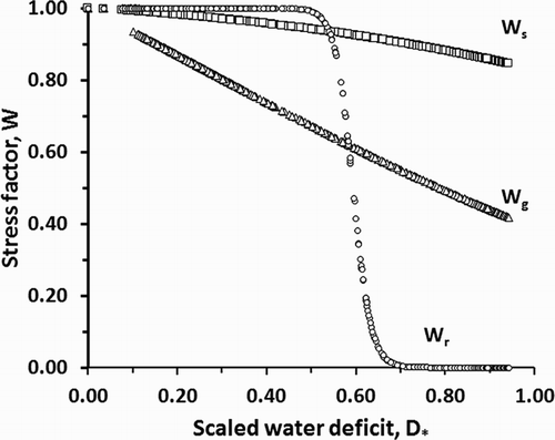
Note that W_g is constrained to unity if D_* has not increased from the day before. In other words, following rain or irrigation, water stress will not affect leaf expansion until all the received water has evaporated.

Experience with the fitting dataset indicated that the development of tillers is stopped abruptly by water stress. The model approximates this behaviour by ceasing increase of leaf numbers and area on tillers 1 and 2 at the first occurrence of (D_*> d_g).

Parameterisation and testing

The model requires values for 28 parameters (Table 2). Some of these were already available from the literature, some were obtained simply by inspection of the fitting dataset, and others had to be fitted by statistical procedures. The fitting procedure sequentially estimated values for the parameters in five groups. When fitting, the parameter values obtained for the preceding groups were held constant. The procedure started by inspecting the fitting dataset and obtaining average values for N_max.mainstem, N_max.tiller1, N_max.tiller2, t_emer, t_silk, η_tiller1, η_tiller2, and Ω (Group 1). For the following groups, parameter values were obtained using a linear programming tool (Solver® in Microsoft Excel®) set to minimise the root mean square (RMS) error of simulation for a different target variable for each group. Group 2 consisted of l_init, l_Ø.mainstem, l_Ø.tiller1, l_Ø.tiller2, α, c_g, and d_g, and the target variable was L. Group 3 consisted of t_s, c_s, and d_s, and the target variable was S. Group 4 consisted of c_r, d_r, σ_Ø, and σ_min, and the target variable was M_p. Finally, Group 5 contained only H_silk and h and the target variable was M_ear.

When fitting or testing, model performance was evaluated using the mean and RMS errors of simulation or prediction, and least-squares linear regressions of observed on simulated data values. Particular attention was also paid to the model’s ability to simulate the time trends in L, S, and G, to check for compensatory errors at different times of the season that might not be apparent in the statistics obtained from the regression analyses.

An initial fit was achieved using a dataset that included much information on the response of sweet corn to water deficits (Dataset 1). The performance of this fit was then tested against independent data (Dataset 2) that compared the responses of sweet corn to different sowing dates. That test indicated that more accurate values were needed for some of the parameters associated with phenology and biomass partitioning. Accordingly, the model was refitted after pooling Datasets 1 and 2. Model performance after this second fit was tested against further independent observations (Dataset 3). The purpose of this test was to evaluate the ability of the model to predict the response of sweet corn yield to a wide range of population densities (ρ) when nutrients were not limiting but water may be. This was a particularly demanding test because Datasets 1 and 2 covered a very narrow range of ρ.

Experimental datasets

Dataset 1 comprised results from an experiment carried out near Lincoln, Canterbury, New Zealand, in 1996–1997 (Stone et al. 2001, 2001). It compared six different water deficit treatments: fully irrigated (FI), severe deficit (FD), moderate early deficit (MED), severe early deficit (SED), moderate late deficit (MLD), and severe late deficit (SLD). The FI treatment received a total of 371 mm of water from rain and irrigation (usually applied weekly to replace evaporative losses); at the other extreme, the FD treatment received only 25 mm. The hybrid was ‘Challenger’ (a shrunken-2 supersweet corn) and ρ was 5.71 m⁻². The leaf area results were recalculated to include tillers, which had been measured but were not included in the calculations of Stone et al. (2001) and Stone et al. (2001). There were twice-weekly non-destructive measurements of leaf numbers (tips and fully expanded leaves), supplemented with two destructive measures of the final leaf area profile. Plant biomass was measured destructively on five occasions during crop growth; the last two of these included separate measurements of ear mass. The model was fitted at the treatment level (there were two replicates per treatment in the original data).

When fitting the model against L(t), it became apparent that the MLD treatment was a strong outlier. Plots of L(t) for the MLD and FI treatments diverged noticeably 4 weeks or so before the MLD treatment was applied. Close examination of the original data revealed that the MLD treatment was anomalous in that none of the six plants selected for leaf area measurement produced more than three leaves on tiller 1 or two leaves on tiller 2. By contrast, plants measured on the FI treatment produced up to 14 and eight leaves on tillers 1 and 2, respectively. This was not commented on by Stone et al. (2001), probably because their analysis concentrated on leaves on the main stem only. Here we did not use the MLD treatment to fit parameters for L and S. However, this treatment was included when fitting parameters for biomass production and partitioning, because those measurements were made on different plants.

Dataset 2 comprised results from an experiment that compared nine different sowing dates through 1999 and 2000 for the ‘Challenger’ hybrid grown near Hastings, Hawke’s Bay, New Zealand (Rogers et al. 2000). The experiment included a tenth sowing date, but the original harvest records for that treatment could not be located. There was one replicate plot per treatment. All treatments received ample irrigation and fertiliser and plant population density was 5.95 m⁻². Plant biomass (including tillers) was measured once close to commercially harvestable maturity. Leaf number and area observations were collected in the same way as for Dataset 1, except that leaf numbers and area were not measured on the tillers. Accordingly, simulated and observed L, S, and G were compared for the main stem only, but the model included leaf area on the tillers when calculating the soil water balance and biomass production.

Dataset 3 summarised results of an experiment that examined the response of the hybrid ‘Challenger’ to p at a single planting date and location (Stone et al. 1998). The crops were grown in the 1997–1998 season on a silty clay loam near Hastings, Hawke’s Bay, New Zealand. There were nine different population treatments, ranging from 3.0 to 14.3 plants m⁻² and two different nitrogen fertiliser treatments (with and without 250 kg N ha⁻¹ applied as urea). There was one replicate plot per treatment, so again, the model was tested and fitted at the treatment level. At the larger plant densities, yields on the non-fertilised treatment were affected by lack of N supply, but there was no sign of this in the fertilised treatment and limitations due to other nutrients were very unlikely (Stone et al. 1998). The model at this stage does not include effects of nutrient supply, and hence here results were used only for the fertilised treatment. However, this experiment was irrigated only once, and the possibility of water stress effects on growth cannot be discounted. The available data consisted of measurements of M_p and M_ear only.

For all datasets, weather observations were made at standard meteorological sites <300 m from the experimental sites, and T_avg was estimated as the average of daily maximum and minimum screen temperatures.

Results

The first fitted version of the model performed very well for L, G, S, M_p, and M_ear in Dataset 1 (Table 3). The mean errors were small and close to zero, indicating little if any systematic bias in the simulated values. The model accounted for 93–98% of the observed variation in these variables, and the regression slopes were generally close to unity. Plots of observed on simulated yield were generally very close to the line of perfect agreement (Figure 2). In general, the model simulated the time trends in L, G, and S very well (Figure 3). It tended to underestimate the later values of L and G for the FI treatment while overestimating them for the MED treatment. It is worth noting that the model substantially overestimated L and G for the MLD treatment from about the time when tillering commenced, but L, S, and G observations from this treatment were not used for model parameterisation (see above).

Figure 2. Comparison of observed with simulated values for L, G, S, M_p, and M_ear for the first fitting (against Dataset 1). The solid lines plotted are those for perfect agreement (slope = 1, intercept = 0). Leaf area data are for the sum of leaves on the main stem and tillers. L, G, and S values are not plotted for the Moderate Late Deficit (MLD) treatment.

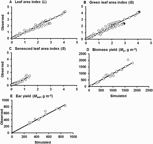
Figure 3. Time courses of simulated and observed leaf areas (L, G, and S) for Dataset 1 after the first fitting of the model. Results are shown for the FI, FD, MED, SED, MLD, and SLD treatments. Note that L, G, and S data for the MLD treatment were not used for model fitting. Values are presented for the sum of main stem and tiller leaves, but Stone et al. (2001) presented only main stem values.

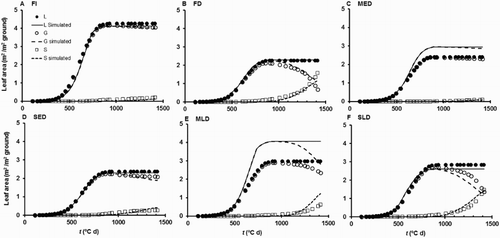
Table 3. Performance of the model against the fitting and test datasets. Tolerances are presented as standard errors (s.e. = SD/√n).

				Regression: observed = slope × simulated		Regression: observed = slope × simulated + intercept
Variable	No. obs.	RMS error	Mean error	Slope ± s.e.	R^2 (%)	Slope ± s.e.	Intercept ± s.e.	r^2
First fitting (Dataset 1)
L	165	0.20	−0.03 ± 0.015	0.98 ± 0.012	98	0.99 ± 0.012	0.0 ± 0.20	98
G	165	0.22	−0.05 ± 0.017	0.97 ± 0.012	97	0.97 ± 0.013	0.0 ± 0.21	97
S	165	0.070	0.017 ± 0.0053	1.01 ± 0.021	93	0.98 ± 0.021	0.02 ± 0.068	93
Mp	30	104	−15 ± 19	1.00 ± 0.039	96	1.04 ± 0.038	−48 ± 109	96
Mear	12	44	5 ± 13	1.00 ± 0.070	94	0.93 ± 0.069	40 ± 59	95
First test (Dataset 2)
L	202	0.25	−0.03 ± 0.017	0.96 ± 0.013	96	0.91 ± 0.012	0.1 ± 0.22	97
G	202	0.27	−0.05 ± 0.019	0.94 ± 0.013	96	0.89 ± 0.013	0.1 ± 0.23	96
S	202	0.063	−0.021 ± 0.0042	0.85 ± 0.24	-	0.50 ± 0.23	0.02 ± 0.059	2
Mp	9	223	92 ± 72	1.1 ± 0.42	71	2.2 ± 0.19	−14531 ± 270	95
Mear	9	224	201 ± 35	1.4 ± 0.44	69	2.0 ± 0.43	−250 ± 220	75
Second fitting (Datasets 1 and 2 pooled)
L	367	0.22	−0.03 ± 0.011	0.975 ± 0.0085	97	0.959 ± 0.0085	0.0 ± 0.21	97
G	367	0.24	0.02 ± 0.012	0.960 ± 0.0092	97	0.940 ± 0.0091	0.1 ± 0.22	97
S	367	0.066	−0.05 ± 0.012	1.01 ± 0.020	87	0.98 ± 0.019	0.02 ± 0.064	88
Mp	39	134	−22 ± 21	1.00 ± 0.042	95	1.07 ± 0.040	−85 ± 137	95
Mear	21	115	10 ± 26	1.0 ± 0.15	61	0.87 ± 0.15	90 ± 150	62
Second test (Dataset 3)
Mp	9	134	−45 ± 45	0.97 ± 0.17	81	1.01 ± 0.18	−52 ± 270	81
Mear	9	101	38 ± 33	1.0 ± 0.22	60	0.8 ± 0.22	170 ± 190	66

RMS = root mean square.

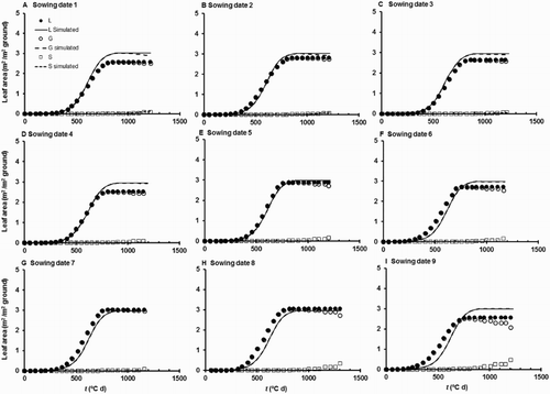
When this first fit of the model was tested on the independent Dataset 2, the predictions of main stem L and G were generally accurate (Table 3, Figure 4). Unlike for Dataset 1, the S values were all very small, and little information can be gleaned from comparing observed and simulated values of these. There was a tendency for the model to overestimate final L values, and to underestimate L slightly for the later sowings during the period of most rapid growth (Figure 5). Simulated values of M_p clustered around the line of perfect agreement (Figure 4), but the RMS error of prediction for M_p and the regressions of observed on simulated were poorer than obtained for Dataset 1 (Table 3). Model performance for M_ear was much worse than for Dataset 1, consistent with the single sowing date of Dataset 1 providing insufficient range to estimate H_silk and h adequately.

Figure 4. Performance of the first fit of the model against independent data for L, G, S, M_p, and M_ear in Dataset 2 (the sowing date experiment of Rogers et al. 2000). Note that the observed and simulated leaf area values refer only to leaves on the main stem. Solid lines are those for perfect agreement.

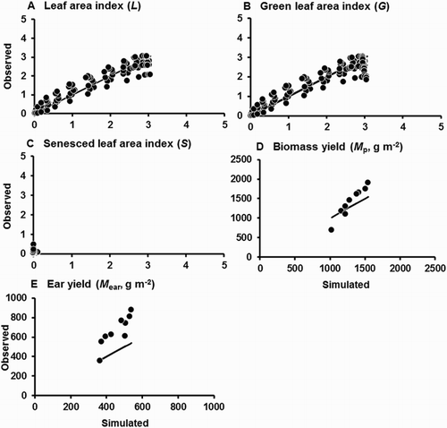
Figure 5. Time courses of simulated and observed main stem leaf areas (L, G, and S) for the nine different sowing date treatments of Dataset 2. This is a test of the first fit of the model. The observed and simulated leaf area values refer only to leaves on the main stem.

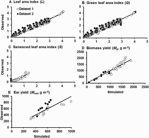
The second fitting of the model (using Datasets 1 and 2 pooled) gave excellent fits for L, S, G, and M_p (Table 3, Figure 6). For these variables, mean errors of simulation were close to zero and the RMS errors were intermediate between the values obtained for the first fitting and the test. The model continued to simulate well the time trends in L, S, and G. Those time trends are not shown because at the scale of figure reproduction here they are indistinguishable from Figures 3 and 5. The tendency remained for the model to underestimate S close to maturity of the last sowing of Dataset 2. The RMS errors and regression analyses indicated that the model performed worst for M_ear, although the regression slopes did not differ significantly from unity, and performance for Dataset 2 was improved compared with the results for the first test.

Figure 6. Performance of the model of sweet corn growth and yield after the second fitting, using pooled data for L, G, S, M_p, and M_ear from Datasets 1 and 2. Solid lines are those for perfect agreement. Note that the leaf area values from Dataset 2 refer only to leaves on the main stem, but those from Dataset 1 include main stem and tillers.

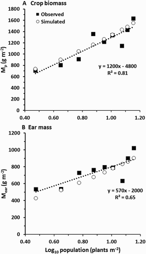
The final test of the model was against Dataset 3. The predicted yields were generally close to the experimental values, and least-squares regression of observed on predicted gave slopes that were not significantly different from 1 (Table 3). As with Datasets 1 and 2, performance was much better for M_p than for M_ear, consistent with the model performing most weakly in describing partitioning of dry matter into ears. For both M_p and M_ear the model successfully predicted that yield would vary linearly with the logarithm of ρ (Figure 7), very closely mimicking the relationships reported by Stone et al. (1998). The model predicted substantial water stress in these crops, with the largest D_* values on the most densely planted treatments (results not shown).

Figure 7. Performance of the model predicting the response of yield (M_p, and M_ear) to plant population (Dataset 3). The dashed lines are least-squares fits for the observed yields only.

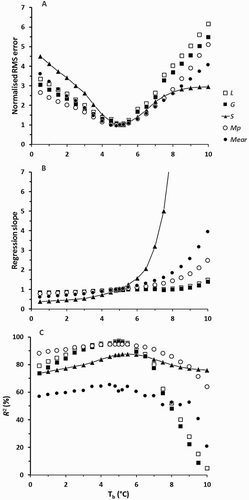
For all those calculations a constant T_b of 5°C was assumed (see Model Description). Model performance for simulation of L, G, M_p, and M_ear was not very sensitive to the assumed value of T_b in the range of 4–6°C (Figure 8). Performance for S was generally much more sensitive, but as noted above the observed values of S were very small.

Figure 8. Sensitivity of model performance to variation in base temperature (T_b) for L, G, S, M_p, and M_ear in Datasets 1 and 2. Three measures of model performance are presented: (a) the RMS error of simulation normalised to the values for T_b = 5°C (the absolute RMS errors for T_b = 5°C are given in Table 3); (b) the slope of a least-squares regression of observed on simulated values; and (c) the percentage of variation accounted for by those same regressions. For clarity, lines are drawn only for the variable S. For each calculation all model parameters except T_b were held at the values previously fitted for Datasets 1 and 2 when T_b = 5°C.

Discussion

Statistically, the model performed very well for leaf area variables and biomass production. This gives confidence that the mechanisms and formulations used are a reliably accurate approximation of reality at the scales of the crop and daily time step. This confidence is supported by examination of some of the fitted parameter values of the model. For example, the stress coefficient W_g fell steadily with increasing D_*, but W_r remained close to 1 until (D_*>0.5), after which it fell abruptly. This behaviour is consistent with observations that leaf area expansion rates are much more sensitive to water deficit than dry matter production rates (Hsiao & Acevedo 1974; Tardieu et al. 1999). The suddenness of the fall in W_g here suggests that, for this hybrid at least, stomatal closure greatly limits net dry matter production once a critical water deficit range is reached.

The model simulated well leaf senescence in response to water deficit, but underestimated late season S in the late sown crops of Dataset 2. This suggests that it is incomplete in its description of S and that further research would be useful. However, extra effort devoted to improving this aspect of the model may not improve predictions of crop yield substantially, because the observed S values were small for all times and treatments within this dataset.

It is worth noting that for Dataset 1 (fitting data) the model simulated well the effects of irrigation treatments on leaf expansion and senescence and M_p. The model also predicted M_p well for Dataset 3 where water stress was highly likely. It described water stress effects in a simple way that is rather more readily implemented than using sequential leaf water potential measurements (Yang et al. 2009) or a time sequence of several different regression relationships between the maximum potential soil water deficit to date and L or S (Stone et al. 2001). This might justify testing the present approach for other crops and situations.

For M_p, accuracy of the model’s performance here appears similar to that reported for CERES-Sweet Corn with crops grown in Florida (Lizaso et al. 2007), although in some situations at least CERES-Sweet Corn seemed to underestimate M_p in the latter third of growth. It is worth noting that in Lizaso et al.’s experiments maximum M_p was c. 1300 g m⁻² compared with c. 2000 g m⁻² here; this difference probably reflected the longer duration of growth under New Zealand conditions.

Sensitivity analyses suggest that model performance for L, G, M_p, and M_ear was not greatly affected by the choice here of T_b = 5°C rather than 6°C as used by Brooking and McPherson (1989). It is worth noting that the results in Figure 8 probably overstate this sensitivity because they reflect model performance when only T_b was varied. If the parameters t_emer, t_mat, t_silk, t_s, α, and Ω had also been adjusted for each individual value of T_b, this would have improved model performance. This emphasises that if users of the model wish to alter the assumptions used to calculate t then those other parameters must be adjusted accordingly.

On the basis of the success of the model presented here in describing leaf area dynamics and dry matter production, further testing and model development is recommended. Testing with other hybrids and environments should be a priority. However, a need for further adjustments to the mechanisms and parameter values is indicated also. Calculation of drainage is necessary to apply the model in many other environments. The method for calculating M_ear also should be improved.

Statistically, the model is least reliable for partitioning of dry matter into ears. In part, this may reflect limitations of using air rather than soil temperature to calculate the time of emergence and the appearance rate of the first six leaves (Stone et al. 1998, 1999), which in turn affect the silking date and the time available thereafter for dry matter to be partitioned into ears. It also reflects a limitation of the available datasets, which have most values of H measured around commercial maturity. Fletcher and Jamieson (2009) have noted that for wheat this same approach can be improved by taking explicitly into account effects of the crop biomass at the start of grain filling, and using a quadratic rather than linear relationship between H and t. Implementing their approach for sweet corn is not simple because sweet corn ears have an appreciable mass before the start of grain filling, and the final yield includes kernels, rachis, and wrapping leaves. Nevertheless, the approach taken here of computing M_ear from harvest index, M_p and t is mechanistically uninformative and can be improved. In its defence, it requires only three readily measured parameters (t_silk, H_silk, and h) for the progression of H(t) and it has considerable empirical support for a range of crops (Muchow 1990; Moot et al. 1996; Robertson et al. 2001). Lizaso et al. (2007) took a different approach. They calculated the fraction of daily net dry matter production that was partitioned into ears as a logistic function of thermal time from silking (using both negative and positive values of the latter). This also is not particularly mechanistic, and depends on five fitted parameters (t for initiation and cessation of ear growth relative to silking, t_silk, and three parameters for the logistic function itself). All of those parameters except t_silk were assumed constant between hybrids (which may need to be checked, as the model depends strongly on them), and they are not especially easy to measure or estimate. An alternative approach yet to be attempted would be to use phenological information to track the initiation of each ear, and allocate a fraction of daily dry matter production to each according to its sink strength. This might rapidly become impractical, however, when ear growth on tillers must be included across a range of stress treatments.

Clearly, further mechanistic development and testing of the harvest index part of the model is needed. This will require experimental data that include many sequential measurements of M_p, M_ear, and ear numbers from before ear initiation to beyond commercial maturity. Further developments are also needed to extend the model to simulate changes in ear quality variables such as kernel moisture content, kernel number, and ear length. The empirical approach to this as used by Lizaso et al. (2007) may be best in the short term, although it will probably need separate fitting exercises for each hybrid and perhaps each environment.

Improving the model’s calculations of t (particularly by switching between soil and air temperatures at appropriate heights), M_p and ear quality parameters, and further research to characterise hybrid differences in model parameters, will give the model considerable utility for forecasting crop performance in industrial settings. Despite its limitations, the present model still has useful predictive ability for identifying how management factors may affect ear yield. This is illustrated by the way that it successfully predicted the patterns of response of M_ear to plant population and sowing date, despite there being negligible variation in plant population in the fitting datasets.

Acknowledgements

I am especially grateful to Peter Stone for allowing access to his original experimental records.

Disclosure statement

No potential conflict of interest was reported by the authors.

Additional information

Funding

This work was part funded by Process Vegetables New Zealand, and MBIE Core Funding administered by the New Zealand Institute for Plant Food & Research Ltd under Programme 1207 (Sustainable and Profitable Vegetable Production Systems).

References

- Aitken AG, Hewett EW. 2016. Fresh facts. Auckland: The New Zealand Institute for Plant & Food Research Ltd; p. 37.
- Aslam T. 2005. Investigations on growth and P uptake characteristics of maize and sweet corn as influenced by soil P status [Unpublished thesis]. Palmerston North: Massey University; p. 222.
- Baird JR, Gallagher JN, Reid JB. 1986. Modelling the influence of flood irrigation on wheat and barley yields; a comparison of nine different models. In: Hillel D, editor. Advances in irrigation. New York: Academic Press; p. 243–306.
- Brooking IR, McPherson HG. 1989. The impact of weather on the scheduling of sweet corn for processing 1. Quantifying the link between rate of development and the environment. New Zealand Journal of Crop and Horticultural Science. 17:19–26. doi: 10.1080/01140671.1989.10428005
- Brown HE, Teixeira EI, Huth NI, Holzworth DP. 2015. The APSIM maize model. [cited May 2016]. Available from: http://www.apsim.info/ApsimxFiles/Maize626.pdf
- Charles-Edwards DA. 1982. Physiological determinants of crop growth. New York: Academic Press; p. 161.
- Fletcher AL, Jamieson PD. 2009. Causes of variation in the rate of increase of wheat harvest index. Field Crops Research. 113:268–273. doi: 10.1016/j.fcr.2009.06.002
- Garcia F, Cruse RM, Blackmer AM. 1988. Compaction and nitrogen placement effect on root growth, water depletion, and nitrogen uptake. Soil Science Society of America Journal. 52:792–798. doi: 10.2136/sssaj1988.03615995005200030035x
- Hsiao TC, Acevedo E. 1974. Plant responses to water deficits, water-use efficiency, and drought resistance. Agricultural Meteorology. 14:59–84. doi: 10.1016/0002-1571(74)90011-9
- Jamieson PD, Martin RJ, Francis GS. 1995. Drought influences on grain yield of barley, wheat, and maize. New Zealand Journal of Crop and Horticultural Science. 23:55–66. doi: 10.1080/01140671.1995.9513868
- Jamieson PD, Zyskowski RF, Li FY, Semenov MA. 2008. Water and N uptake and responses in models of wheat, potatoes and maize. In: Ma L, Ahuja LR, Bruulsema TW, editors. Quantifying and understanding plant nitrogen uptake systems modeling. Boca Raton (FL): CRC Press; p. 127–146.
- Johns G, Smith R. 1975. Accuracy of soil water budgets based on a range of relationships for the influence of soil water availability on actual water use. Australian Journal of Agricultural Research. 26:871–883. doi: 10.1071/AR9750871
- Jones JW, Hoogenboom G, Porter CH, Boote KJ, Batchelor WD, Hunt LA, Wilkens PW, Singh U, Gijsman AJ, Ritchie JT. 2003. The DSSAT cropping system model. European Journal of Agronomy. 18:235–265. doi: 10.1016/S1161-0301(02)00107-7
- Lemeur R, Blad BL. 1974. A critical review of light models for estimating the shortwave radiation regime of plant canopies. Agricultural Meteorology. 14:255–286. doi: 10.1016/0002-1571(74)90024-7
- Lizaso J, Boote K, Cherr C, Scholberg J, Casanova J, Judge J, Jones J, Hoogenboom G. 2007. Developing a sweet corn simulation model to predict fresh market yield and quality of ears. Journal of the American Society for Horticultural Science. 132:415–422.
- Monteith JL. 1977. Climate and the efficiency of crop production in Britain. Philosophical Transactions of the Royal Society B: Biological Sciences. 281:277–294. doi: 10.1098/rstb.1977.0140
- Moot DJ, Jamieson PD, Henderson AL, Ford MA, Porter JR. 1996. Rate of change in harvest index during grain-filling of wheat. The Journal of Agricultural Science. 126:387–395. doi: 10.1017/S002185960007547X
- Muchow RC. 1990. Effect of high temperature on grain-growth in field-grown maize. Field Crops Research. 23:145–158. doi: 10.1016/0378-4290(90)90109-O
- Olsen JK, McMahon CR, Hammer GL. 1993. Prediction of sweet corn phenology in subtropical environments. Agronomy Journal. 85:410–415. doi: 10.2134/agronj1993.00021962008500020044x
- Pages L, Jordan MO, Picard D. 1989. A simulation model of the three-dimensional architecture of the maize root system. Plant and Soil. 119:147–154. doi: 10.1007/BF02370279
- Priestley CHB, Taylor RJ. 1972. On the assessment of surface heat flux and evaporation using large-scale parameters. Monthly Weather Review. 100:81–92. doi: 10.1175/1520-0493(1972)100<0081:OTAOSH>2.3.CO;2
- Reid JB. 1990. Growth and water use of faba beans (Vicia faba) in a sub-humid climate. II: simulation analysis of crop responses to drought. Field Crops Research. 23:19–38. doi: 10.1016/0378-4290(90)90094-R
- Reid JB, English JM. 2000. Potential yield in carrots: theory, test and an application. Annals of Botany 85:593–605. doi: 10.1006/anbo.2000.1108
- Reid JB, Hashim O, Gallagher JN. 1984. Relations between available and extractable soil water and evapotranspiration from a bean crop. Agricultural Water Management. 9:193–209. doi: 10.1016/0378-3774(84)90002-7
- Reid JB, Stone PJ, Pearson AJ, Cloughley C, Wilson DR. 1999. ‘The Maize Calculator’ – a simple system for predicting fertiliser nitrogen requirements of maize. Agronomy New Zealand. 29:73–74.
- Ritchie JT. 1972. Model for predicting evaporation from a row crop with incomplete cover. Water Resources Research. 8:1204–1213. doi: 10.1029/WR008i005p01204
- Ritchie JT. 1973. Influence of soil water status and meteorological conditions on evaporation from a corn canopy. Agronomy Journal. 65:893–897. doi: 10.2134/agronj1973.00021962006500060014x
- Ritchie JT. 1981. Water dynamics in the soil-plant-atmosphere system. Plant and Soil. 58:81–96. doi: 10.1007/BF02180050
- Robertson MJ, Silim S, Chauhan YS, Ranganathan R. 2001. Predicting growth and development of pigeonpea: biomass accumulation and partitioning. Field Crops Research. 70:89–100. doi: 10.1016/S0378-4290(01)00125-3
- Rogers BT, Sorensen I, Stone PJ. 1999. Is sweet corn just another maize hybrid? Agronomy New Zealand. 29:87–90.
- Rogers BT, Stone PJ, Shaw SR, Sorensen IB. 2000. Effect of sowing time on sweet corn yield and quality. Agronomy New Zealand. 30:55–61.
- Sinclair TR, Muchow RC. 1995. Effect of nitrogen supply on maize yield: I. Modeling physiological responses. Agronomy Journal. 87:632–641. doi: 10.2134/agronj1995.00021962008700040005x
- Stapper M, Arkin GF. 1980. CORNF: a dynamic growth and development model for maize (Zea mays L.). Program and model documentation No. 80-2. Temple: Texas Agricultural Experiment Station, Blackland Research Centre; p. 91.
- Stone PJ, Sorenson IB, Reid JB. 1998. Effect of plant population and nitrogen fertiliser on yield and quality of super sweet corn. Journal of the Royal Society of New Zealand. 28:1–37. doi: 10.1080/03014223.1998.9517553
- Stone PJ, Sorensen I, Jamieson PD. 1998. Soil temperature affects growth and development of maize. Proceedings Agronomy Society of New Zealand. 28:7–8.
- Stone PJ, Sorensen IB, Jamieson PD. 1999. Effect of soil temperature on phenology, canopy development, biomass and yield of maize in a cool-temperate climate. Field Crops Research. 63:169–178. doi: 10.1016/S0378-4290(99)00033-7
- Stone PJ, Wilson DR, Jamieson PD, Gillespie RN. 2001. Water deficit effects on sweet corn. II. Canopy development. Australian Journal of Agricultural Research. 52:115–126. doi: 10.1071/AR99145
- Stone PJ, Wilson DR, Reid JB, Gillespie RN. 2001. Water deficit effects on sweet corn. I. Water use, radiation use efficiency, growth and yield. Australian Journal of Agricultural Research. 52:103–113. doi: 10.1071/AR99146
- Tardieu F, Granier C, Muller B. 1999. Modelling leaf expansion in a fluctuating environment: are changes in specific leaf area a consequence of changes in expansion rate?. New Phytologist. 143:33–43. doi: 10.1046/j.1469-8137.1999.00433.x
- Wilson DR, Muchow RC, Murgatroyd CJ. 1995. Model analysis of temperature and solar radiation limitations to maize potential productivity in a cool climate. Field Crops Research. 43:1–18. doi: 10.1016/0378-4290(95)00037-Q
- Yang Y, Timlin DJ, Fleisher DH, Kim SH, Quebedeaux B, Reddy VR. 2009. Simulating leaf area of corn plants at contrasting water status. Agricultural and Forest Meteorology. 149:1161–1167. doi: 10.1016/j.agrformet.2009.02.005