Global long-term monitoring of the ozone layer – a prerequisite for predictions

Abstract

Although the Montreal Protocol now controls the production and emission of ozone depleting substances, the timing of ozone recovery is unclear. There are many other factors affecting the ozone layer, in particular climate change is expected to modify the speed of re-creation of the ozone layer. Therefore, long-term observations are needed to monitor the further evolution of the stratospheric ozone layer. Measurements from satellite instruments provide global coverage and are supplementary to selective ground-based observations. The combination of data derived from different space-borne instruments is needed to produce homogeneous and consistent long-term data records. They are required for robust investigations including trend analysis. For the first time global total ozone columns from three European satellite sensors GOME (ERS-2), SCIAMACHY (ENVISAT), and GOME-2 (METOP-A) are combined and added up to a continuous time series starting in June 1995.

On the one hand it is important to monitor the consequences of the Montreal Protocol and its amendments; on the other hand multi-year observations provide the basis for the evaluation of numerical models describing atmospheric processes, which are also used for prognostic studies to assess the future development. This paper gives some examples of how to use satellite data products to evaluate model results with respective data derived from observations, and to disclose the abilities and deficiencies of atmospheric models. In particular, multi-year mean values derived from the Chemistry-Climate Model E39C-A are used to check climatological values and the respective standard deviations.

1. Introduction

The depletion of the stratospheric ozone layer in recent years, particularly above Antarctica during spring time, i.e. the ozone hole, has been one of the most obvious changes observed in Earth's atmosphere. The discovery of the ozone hole in 1984 (Chubachi 1985, Farman et al. 1985) was a surprising issue as well as the continuous reduction of ozone concentrations in the succeeding years. Sustainable global observations with space-borne instruments play an essential role in explaining and understanding the global changes of stratospheric ozone. Although the Montreal Protocol (UNEP 2006) and its amendments have now regulated the production and release of ozone depleting substances (ODSs), e.g. chlorofluorocarbons (CFCs), which will prevent a further thinning of the ozone layer and lead to a gradual recovery in the next decades, there are still open questions with regard to the beginning of ozone recovery and the timing of full recovery. To answer these questions not only are further continuous measurements needed but also numerical models describing relevant atmospheric processes and their mutual effects. Atmospheric models, in particular those considering the interaction of climate and atmospheric chemistry, i.e. so-called Chemistry-Climate Models (CCMs), have been developed recently to identify and quantify relevant processes affecting the ozone layer. Predictions of future changes of stratospheric ozone and climate are required for international assessment reports of the World Meteorological Organisation (WMO) and the Intergovernmental Panel of Climate Change (IPCC) as part of the Montreal Protocol (UNEP 2006) and the Kyoto Protocol (Kyoto 1998), respectively.

Beside the impact of ozone depleting substances, natural fluctuations (e.g. the 11-year solar activity cycle, the equatorial quasi-biennial oscillation of the lower stratospheric zonal wind (QBO), and volcanic eruptions) are significantly affecting the thickness of the ozone layer. Moreover, climate change due to increases in greenhouse gas concentrations will influence stratospheric dynamics and chemistry, and therefore the ozone layer. A better understanding of radiative, dynamical, and chemical processes and the interaction between climate change and atmospheric chemistry is highly necessary for reliable projections of future stratospheric ozone levels. The basis for reliable model assessments is a review of model data generated for the past time with available observations. Only models which have demonstrated their capability to reproduce adequately recent developments can provide reasonable estimates of future behaviour.

The present paper demonstrates the importance of a consistent multi-year dataset of total ozone which is composed from different satellite instruments. Merging their data is a key problem concerning the estimation of long-term ozone trends as an accuracy of better than 1% per decade is desired. Important factors such as spatial coverage, instrument drifts, record continuity, and long-term calibration stability are constricted when satellite data are considered. In this study we present an example of using merged satellite ozone time series for the validation of global atmospheric models which are used for predictions of the future ozone evolution and its expected recovery.

2. Total ozone datasets

Covering the period from mid 1995 to 2008 monthly means of total ozone columns from three different data sources were used in this study: homogenized measurements from three different satellite instruments, modelled data from a Chemistry-Climate Model, as well as ground-based measurements from 79 individual ground stations equipped with Dobson or/and Brewer instruments.

2.1 Satellite measurements

This work uses global ozone data provided by three European satellite instruments for the time period from June 1995 to May 2008. Measurements from the Global Ozone Monitoring Experiment (GOME) onboard the ESA satellite ERS-2 launched in April 1995 (Burrows et al. 1999) are still available, but global coverage was lost in June 2003. This atmospheric composition data record was extended through May 2008 by measurements from the Scanning Imaging Absorption spectrometer for Atmospheric CHartographY (SCIAMACHY) onboard the ESA satellite ENVISAT launched in February 2002 (Bovensmann et al. 1999, Gottwald et al. 2006), and GOME-2 onboard EUMETSAT's MetOp-A satellite launched in October 2006 (Callies et al. 2000). The data are merged based upon comparisons during the overlap period from July 2002 to May 2008 for GOME and SCIAMACHY, and from March 2007 to May 2008 for GOME and GOME-2, respectively. In both cases, GOME data are considered as reference standard. The algorithm used for the adjustment of SCIAMACHY and GOME-2 is described in detail in Section 3.

Note that two other European satellites also provide ozone data in this time period, but they are not used in this work. The Michelson Interferometer for Passive Atmospheric Sounding (MIPAS) onboard ENVISAT (Fischer and Oelhaf 1996) and the Ozone Monitoring Instrument (OMI) onboard the NASA satellite AURA launched in July 2004 (Levelt et al. 2006). Data from OMI could be used to extend the measurement time series and/or to improve the statistics. Ozone vertical distribution from MIPAS may provide supplementary information about the evolution of ozone concentrations in different layers of the atmosphere (Cortesi et al. 2007).

GOME, SCIAMACHY, and GOME-2 are passive remote sensing instruments whose primary objective is the determination of the amounts and distributions of atmospheric constituents, such as trace gases, aerosols, and clouds. All three instruments are spectrometers which are designed to measure sunlight reflected, and scattered by the Earth's atmosphere or surface in the ultraviolet, visible, and near-infrared wavelength region. The ERS-2, ENVISAT, and MetOp-A satellites fly in sun-synchronous and near polar orbits (inclination 98.5°) at a height of about 790 km. Each orbit takes ∼100 minutes which implies a completion of ∼14 orbits per day. Equator crossing times in descending node are at 10:30 a.m. local time (LT) for GOME, 10:00 a.m. LT for SCIAMACHY, and 09:30 a.m. LT for GOME-2, respectively. All three instruments provide atmospheric measurements within about one hour. This relatively small time difference facilitates the combination of the retrieval results. An overview of the most important instrument properties and viewing geometries is given in table 1.

Table 1. Satellite instrument properties

Parameter	GOME	SCIAMACHY	GOME-2
Data Availability	06/1995-today^a	07/2002-today	03/2007-today
Spectral Coverage	240–790 nm	240–2380 nm	240–790 nm
Spectral Resolution	0.2–0.4 nm	0.2–1.5 nm	0.2–0.4 nm
PMD Coverage	3 p-PMD^b 300–800 nm	6 p-PMD 320–2380 nm	15 p-PMD and 15 s-PMD^c 310–790 nm
Viewing Geometries	nadir	nadir, limb, occultation	nadir
Ground Pixel Size	320 × 40 km^2	60 × 30 km^2	40 × 80 km^2
Swath Width	960 km	960 km	1920 km
Equator Crossing	10:30 a.m. LT^d	10:00 a.m. LT	09:30 a.m. LT
Global Coverage	3 days	6 days	almost daily
^aNo global coverage since June 2003.
^bp-PMD: measures light polarized perpendicular to the optical plane.
^cs-PMD: measures light polarized parallel to the optical plane.
^dLT: Local Time

GOME observes the atmosphere in across-track nadir sounding mode using four spectral channels covering the wavelength region from 240 nm to 793 nm. Part of the light is branched out and recorded with three Polarization Measurement Devices (PMDs) that measure the amount of light polarized parallel to the instrument slit. In normal viewing mode, the GOME ground pixels have a footprint size of 320 km by 40 km covering a swath width of 960 km. Global coverage is achieved at the equator within three days.

GOME measurements have been available since the end of June 1995, but as a result of a permanent tape recorder failure on the ERS-2 satellite, global coverage was lost in June 2003. Since then the availability of GOME data coverage is limited to the north Atlantic sector and north polar region, but additional ground stations have been brought online to increase the data gathering abilities of the satellite.

SCIAMACHY measures irradiance and radiance spectra in the ultraviolet, visible and near-infrared from 240 nm to 2380 nm. The instrument is alternating the limb- and nadir-viewing modes and achieves a global coverage in 6 days. The total ozone columns are retrieved by making use of the nadir spectra with a spatial resolution of 30 km by 60 km.

In October 2006 the first of a series of the European operational meteorological satellites (MetOp) has been launched. One instrument on-board MetOp is GOME-2, an enhanced version of GOME covering the same spectral range, 240–790 nm. GOME-2 measures the polarization in two planes using fifteen broad channels for each plane. GOME-2 has a spatial resolution of 80 km by 40 km and a larger swath width of 1920 km, resulting in a daily coverage at mid-latitudes. Another two MetOp satellites will be launched in the coming years extending in this way the GOME/SCIAMACHY/GOME-2 atmospheric composition data record to cover a total of 25 years.

The GOME Data Processor (GDP) version 4.x is the operational algorithm for the trace gas column retrievals from GOME, SCIAMACHY (UV-VIS nadir) and GOME-2. GDP 4.x is a fitting algorithm for the generation of total column amounts of ozone, NO₂, BrO, SO₂, H₂O, HCHO, and OClO. The GDP algorithm, based on the scientific algorithm GDOAS, has two major steps: the Differential Optical Absorption Spectroscopy (DOAS) least-squares fitting for the trace gas slant column, followed by the computation of a suitable Air Mass Factor to make the conversion to the vertical column density (Van Roozendael et al. 2006). Cloud information (fractional cover, cloud-top height and cloud-top albedo) is derived directly from the instrument measurements using the Optical Cloud Recognition Algorithm (OCRA) and the Retrieval Of Cloud Information by Neural Networks (ROCINN) algorithm (Loyola et al. 2007).

The operational GOME and GOME-2 total ozone products (GDP 4.x) are used in this paper. The SCIAMACHY total ozone columns used in this work are retrieved using SDOAS, an adaption of the algorithm GDOAS to the SCIAMACHY instrument (Lerot et al. 2008). SDOAS has been implemented in the ESA SCIAMACHY Ground Processor SGP version 3. To correct for cloud contamination, SDOAS ingests the parameters derived off-line by the updated Fast Retrieval Scheme for Clouds from the Oxygen A-band (FRESCO+) algorithm (Koelemeijer et al. 2001, Wang et al. 2008). In the operational environment, the cloud parameters are retrieved using the OCRA algorithm (Loyola 2000, 2004) and the Semi-Analytical Cloud Retrieval Algorithm (SACURA) (Kokhanovsky et al. 2008).

GDP 4.x has been used operationally for GOME since 2004 and for GOME-2 (Valks and Loyola 2008) since the start of data dissemination in early 2007. SGP 3.x is being used operationally for SCIAMACHY since 2006.

Quality assessment of the operational products is guaranteed with a continuous geophysical validation using ground-based and other satellite measurements. The average agreement of GOME, SCIAMACHY and GOME-2 total ozone products with ground-based and other satellite ozone column measurements is at the ‘percent level’ (Balis et al. 2007b, 2008).

The long-term stability of the GOME total ozone record, which is a key consideration for trend analysis, is demonstrated in figure 1. Monthly mean ozone differences between GDP 4.1 and Brewer measurements at Hohenpeissenberg (48° N, 11° E) are shown for the 12 year period from July 1995 to November 2007. A sine function has been fitted to the time series in order to highlight seasonal variations in the differences. The amplitude of these variations is about 0.5% and the mean bias is 0.3%. The long-term stability of GOME and the absence of any significant time-dependent bias are apparent. Furthermore, these results suggest that the DOAS algorithm is not strongly influenced by the degradation of the instrument (see also Van Roozendael et al. 2004, their figures 4 and 5).

Figure 1. GDP v4.1 – Hohenpeissenberg (48° N, 11° E) Brewer monthly mean ozone differences from July 1995 to November 2007. A sinusoidal fit to the time series (thick solid line) highlights the size of seasonal variations in the differences (amplitude: 0.5%). The mean bias over the 12 year period is 0.3%.

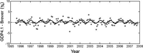
Figure 4. Monthly mean ozone values averaged over 60°N to 60°S for the merged data set including GOME, as well as adjusted SCIAMACHY and GOME-2 data (solid black, grey, and broken black lines respectively). Additionally, the original SCIAMACHY data (dashed grey line) and GOME-2 data (dashed black line) are plotted.

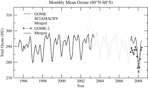
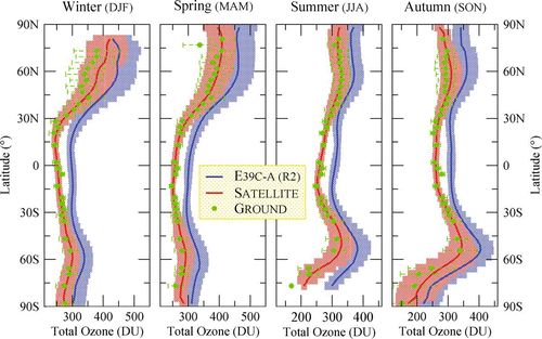
Figure 5. Zonal mean (June 1995 to May 2008) total ozone values for each season from satellite instruments (mean values in red with standard deviations as background surfaces), ground-based measurements (green points with mean values and standard deviations), and results from E39C-A (blue curves with mean and standard deviation).

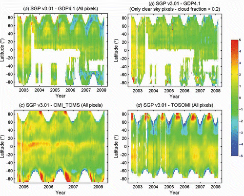
Lerot et al. (2008) have compared the SCIAMACHY total ozone columns from SGP v3.01 to other products derived from different algorithms and/or instruments. Figure 2 summarizes these comparisons. Figures 2(a) and (b) illustrate the relative differences of the SGP O₃ columns with respect to the GDP v4.1 columns, by considering all pixels or only clear sky pixels respectively. As the retrieval algorithms in both operational processors are similar, the O₃ columns from the two instruments are very consistent, especially for the clear sky pixels for which the differences generally are close to 0%. It was shown that larger differences may happen for cloud contaminated pixels due to the different cloud algorithms used in the two processors. The comparisons with OMI columns retrieved with the Total Ozone Mapping Spectrometer (TOMS) v8.5 algorithm and with the scientific SCIAMACHY retrieval algorithm TOSOMI (Total Ozone retrieval scheme for SCIAMACHY based on the OMI DOAS algorithm) show that the overall agreement is satisfactory with differences generally lower than 2% except in specific conditions such as ozone hole, or very high solar zenith angles (figures 2c and d ). Also, Lerot et al. (2008) have highlighted a slight decreasing trend in the SCIAMACHY total O₃ columns with an amplitude less than 0.5% per year. The origin of this trend remains unclear but is to look for in the instrumental degradation or in level 0-to-1 processing inaccuracies.

Figure 2. Latitudinal and temporal dependencies of the relative differences of the SGP 3.01 total O₃ columns with respect to: (a) the GDP 4.1 columns (all pixels considered); (b) the GDP 4.1 columns (only clear sky pixels considered); (c) the OMI columns retrieved with the TOMS v8.5 algorithm (all pixels considered); (d) the TOSOMI columns (all pixels considered).

2.2 E39C-A

Over the last 10 years several CCMs have been developed and applied to investigate recent changes of stratospheric ozone concentrations (e.g. Eyring et al. 2006), and to simulate the future evolution of the ozone layer (e.g. Eyring et al. 2007). In this paper we concentrate on results of the CCM E39C-A (Stenke et al. 2008) which is an upgraded version of the CCM E39C (Dameris et al. 2005) employing the fully Lagrangian advection scheme ATTILA (Reithmeier and Sausen 2002) for tracer transport. ATTILA is strictly mass conserving and numerically non-diffusive. Water vapour, cloud water and chemical trace species are advected by ATTILA instead of the operational semi-Lagrangian advection scheme of Williamson and Rasch (1994) which has been used in the previous model version E39C. The model system E39C (Hein et al. 2001) has been applied for several chemistry-climate studies based on time-slice (e.g. Schnadt et al. 2002), Grewe et al. 2004, Stenke and Grewe 2005) as well as transient simulations (Dameris et al. 2005, 2006, Grewe 2007).

E39C-A consists of the dynamic part E39 and the chemistry module CHEM. E39 is a spectral general circulation model, based on the climate model ECHAM4 (Roeckner et al. 1996). It has a vertical resolution of 39 levels up to the top layer centred at 10 hPa (Land et al. 2002). A spectral horizontal resolution of T30 (≈6° isotropic resolution) is used. The corresponding Gaussian transform grid, on which the tracer transport, model physics and chemistry are calculated, has a mesh size of approximately 3.75° × 3.75°. The chosen time step is 24 min.

The chemistry module CHEM (Steil et al. 1998) is based on the family concept. It includes stratospheric homogeneous and heterogeneous ozone chemistry and the most relevant chemical processes for describing the tropospheric background chemistry with 107 photochemical reactions, 37 chemical species and four heterogeneous reactions on polar stratospheric clouds (PSCs) and on sulphate aerosols. In contrast to previous studies with E39C the present model version considers a parameterisation for bromine chemistry (ClO/BrO-cycle) based on the photolysis of Cl₂O₂ (based on Rex et al. 2003). To account for the effects of twilight stratospheric ozone chemistry the photolysis at solar zenith angles up to 93° has been implemented (Lamago et al. 2003). Net heating rates and photolysis rates are calculated on-line from the modelled distributions of the radiatively active gases O₃, CH₄, N₂O, H₂O and CFCs, and the actual cloud distribution. More details about the CCM E39C-A are given in Stenke et al. (2008).

In the present study two transient model simulations (i.e. using transient boundary conditions) with E39C-A have been used, R1 and R2. The R1 simulation covers the years from 1960 to 2004, the R2 model simulation covers the extended period from 1960 to 2050. Both model simulations include various natural and anthropogenic forcings like the 11-year solar cycle, the QBO, chemical and direct radiative effects of major volcanic eruptions, and the increase in greenhouse gas concentrations. The QBO is forced externally by a linear relaxation (‘nudging’) of the simulated zonal winds in the equatorial stratosphere to a constructed QBO time series which follows observed equatorial zonal wind profiles (Giorgetta and Bengtsson 1999). This assimilation is applied between 20° N and 20° S from 90 hPa up to the model top layer. The relaxation time scale is 7 days within the QBO core domain. Outside the core region the time scale depends on latitude and pressure (Giorgetta and Bengtsson 1999). The influence of the 11-year solar cycle on photolysis is parameterized according to the intensity of the 10.7 cm radiation of the sun (Lean et al. 1997, data available via http://www.drao.nrc.ca/icarus/www/daily.html). The impact of solar activity on short-wave radiative heating rates is considered on the basis of changes of the solar constant (Dameris et al. 2005, their table 2).

For the past the boundary conditions are based on observational data. Detailed information about the experimental set-up is given by Stenke et al. (2008). For the future, we introduced some changes which are described in the following: the QBO-phases observed in the past are consistently continued. The solar activity signal (i.e. the intensity of the 10.7 cm radiation) observed between 1977 and 2007 is continually repeated until 2050. Furthermore, we do not introduce a major volcanic eruption in the future. The most important change affects the prescribed sea surface temperatures (SSTs). In the R1 simulation the SSTs were prescribed as monthly means following the global sea ice and SST dataset HadISST1 derived from observations (Rayner et al. 2003). To avoid a discontinuity at the transition point from past to future, in R2 we use a continuous dataset derived from a coupled atmosphere ocean model containing SST and sea ice data for the years from 1960 to 2050. The data are taken from the HadGEM1 model, provided by the UK Met Office Hadley Centre (Johns et al. 2006). The HadGEM1 simulations used are transient simulations with prescribed anthropogenic forcing as observed in the past, and following the SRES-A1B scenario in the future (for details on the simulations see Stott et al. 2006).

2.3 Ground-based measurements

In this work, archived total ozone column measurements from the World Meterological Organization (WMO) – Global Atmosphere Watch (GAW) network routinely deposited at the World Ozone and Ultraviolet Radiation Data Centre (WOUDC) in Toronto, Canada (http://www.woudc.org) were utilized for the ground-based measurements reference. The WOUDC archive contains total ozone column data mainly from Dobson and Brewer UV spectrophotometers as well as from M-124 UV filter radiometers from the early 1950s onwards. In general, spatial and temporal coincidences offered by the Dobson and Brewer networks are sufficient to cover a wide geographical extent for the validation of a satellite sensor, however, with better coverage over land with respect to sea and over the northern hemisphere compared to the southern hemisphere. Total ozone column data from a large number of stations have already been used extensively both for trend studies (e.g. World Meteorological Organization 1998, 2002, 2006) as well as for validation of satellite total ozone data (e.g. Lambert et al. 1999, Fioletov et al. 1999, Lambert et al. 2000, Bramstedt et al. 2003, Labow et al. 2004, Weber et al. 2005, Balis et al. 2007b). Van Roozendael et al. (1998) have shown that Dobson and Brewer data can agree within 1% when the major sources of discrepancy are properly accounted for. Dobson measurements suffer from a temperature dependence of the ozone absorption coefficients used in the retrievals which might account for a seasonal variation in the error of ±0.9% in the middle latitudes and ±1.7% in the Arctic, and for systematic errors of up to 4% (Bernhard et al. 2005). The error of individual total ozone measurements for a well maintained Brewer instrument is about 1% (e.g. Kerr et al. 1988). Despite the similar performance between the Brewer and Dobson stations, small differences within ±0.6% are introduced due to the use of different wavelengths and different temperature dependence for the ozone absorption coefficients (Staehelin et al. 2003). Dobson and Brewer instruments might also suffer from long-term drift associated with calibration changes. Additional problems arise at solar elevations lower than 15°, for which diffuse and direct radiation contributions can be of the same order of magnitude.

To prepare the ground-based dataset for comparison with satellite measurements, we investigated the quality of the total ozone values of each station and instrument that deposited data at WOUDC for any time period after 1995. For detailed discussion on the selection process and the exclusion procedures please refer to Balis et al. (2007a). Using the methodology described in great detail in that publication, 32 Brewer and 47 Dobson stations were considered as potentials for the comparisons with GOME, SCIAMACHY, and GOME-2 total ozone column data. These stations are sorted with decreasing latitude and listed in Appendix A in table A1 for northern high and mid latitudes and in table A2 for low latitudes and the southern hemisphere, respectively.

The monthly mean averages were then created using the daily comparison measurements with two different sets of only coincident datasets being considered: the monthly mean and associated standard deviation of the ground-based measurements and the equivalent one for the satellite measurements. Due to the differences in time-span and spatial resolution between the three satellite datasets considered, not all of the above shown ground-based stations were utilized in the comparisons of all three satellite instruments.

3. Merged GOME/SCIAMACHY/GOME-2 total ozone time series

The single GOME, SCIAMACHY, and GOME-2 ozone total column measurements are averaged to monthly means for each satellite using a grid of 0.33° × 0.33°. The satellite measurements are first projected on to this regular grid using the Lambert Azimuthal equal-area projection, and the normalized area of the intersecting polygon (n_{i_area}) is computed. A daily composite is then created from forward scan measurements only (the backward scan measurements cover the same area as the forward scans, but with bigger ground pixel size). For each point of the globe only one observation is used per day. The metric m is computed for all grid points having more than one satellite observation per day

(1)

where SZA and VZA are the Sun and Viewing Zenith Angles, respectively. The measurement with the smallest m, i.e. the one with the smallest geometrical air mass factor and the largest normalized intersecting area, goes into the daily composite. The monthly means are finally computed as the area-weighted average of the daily composites, following the algorithm proposed by West (1979). The area_weight is computed from the normalized intersecting area and the geographical area as a function of latitude φ of each grid point as

(2)

This area_weighting is important for the computation of the latitudinal means.

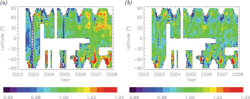
As a result of the analysis in section 2.1, we decided to use the very stable long-term ozone time series from GOME as a reference standard, whereas SCIAMACHY and GOME-2 data will be adjusted to GOME in periods of instrument overlap. The temporal evolution and spatial variation of the differences between SCIAMACHY and GOME has been investigated for the period from July 2002 to January 2008 in terms of 1° latitudinal means. The ratio GOME/SCIAMACHY total ozone is depicted in the top panel of figure 3. White areas since mid 2003 denote missing GOME data due to the tape recorder failure. The drift of SCIAMACHY data compared to GOME is clearly visible. In 2002–2003 SCIAMACHY ozone values are about 2% larger than GOME data (dark green and blue areas). Until 2006 the ratio obverts and SCIAMACHY ozone data become smaller than GOME retrieval results (yellow and red areas in northern and southern mid latitudes). In both hemispheres, poleward of 50°, very large ratios are found around the polar night under high solar zenith angle conditions.

Figure 3. Ratio GOME/SCIAMACHY 1°latitudinal monthly total ozone columns before (a) and after (b) adjustment of SCIAMACHY according to equations (3(3))(3) (4) (5) (6) (7)–(8)(8). See text for more details.

The adjustment applied to SCIAMACHY data comprises of two parts, a basic latitudinal correction for each month of the year, and a time-dependent correction for each individual month from July 2002 to January 2008, which is then an offset averaged over latitude from 60° N to 60°S. This is in contrast to the approach used for the combination of several TOMS (Total Ozone Mapping Spectrometer) and SBUV(/2) (Solar Backscatter Ultraviolet) instrument data records, where temporal and/or latitudinal variations in the instrument differences are neglected (Miller et al. 2002, Stolarski and Frith 2006). The merged ozone dataset (MOD) which combines Version 8 total ozone measurements from TOMS (Nimbus 7 and Earth Pobe (EP)), SBUV/SBUV2 (Nimbus 7, and NOAA 9/11/16), and recently OMI (Ozone Monitoring Instrument on EOS-AURA)—available via http://code916.gsfc.nasa.gov/Data_services/merged---is composed using the temporal mean of the differences averaged from 50° S – 50° N over the available overlap period as adjustment to each dataset, where EP TOMS data from 1996 through mid-1999 are selected as the reference standard (Stolarski and Frith 2006). Temporal variation of the differences between the instrument systems comparable to the SCIAMACHY drift (see left panel of figure 3) is also neglected for the cohesive SBUV(/2) time series (Miller et al. 2002).

For the latitudinal correction, monthly averages of the differences between SCIAMACHY and GOME have been calculated as a function of latitude φ as:

(3)

with month m from January to December, year y from 2002 to 2008, and m_y from July 2002 to January 2008. The latitudinal correction is then a third-order polynomial fit over latitude for each of those 12 monthly differences as:

(4)

As the differences between SCIAMACHY and GOME, as well as SCIAMACHY and OMI, respectively, show some drift during the last six years (see figure 2), whereas the GOME data remain stable compared to ground-based data (see figure 1), the adjustment requires also a time-dependent component. For this temporal contribution to the overall correction the mean difference between GOME and SCIAMACHY over all available N _φ latitudes from 60° N to 60° S is computed for each month m_y as:

(5)

This difference is compared to the monthly mean difference over all years for the same latitude range:

(6)

with month m from January to December. The time-dependent correction (or offset) is then given by:

(7)

Finally the overall adjustment for SCIAMACHY data is the sum of the latitudinal correction and the time-dependent offset:

(8)

Figure 3(b) shows the ratios GOME/SCIAMACHY with adjustment applied to SCIAMACHY according to 3–8. The general agreement is much better, and the drift has diminished, but some extreme values poleward of 50° still remain.

The differences between GOME and GOME-2 1°zonal ozone means are more homogeneous than the differences between SCIAMACHY and GOME. GOME-2 ozone columns are on average 2–3% lower than GOME ozone values. As the overlap period between GOME-2 and GOME is limited to 15 months from March 2007 to May 2008, the GOME-2 adjustment comprises one part only. For each month a third order polynomial fit over latitude from 90° N to 90° S is performed similar to the SCIAMACHY adjustment, and then applied as correction factor for GOME-2 columns. With extension of the time series, also for GOME-2 a two-step time-dependent correction is planned.

Finally, the complete and homogenized ozone time series comprises GOME data from June 1995 to May 2003, SCIAMACHY data from June 2003 to February 2007, and GOME-2 data from March 2007 to May 2008. Although SCIAMACHY data have already been available since July 2002, we used GOME data until May 2003, because of (1) the excellent GOME data stability and (2) the final flight conditions of SCIAMACHY, which were achieved in January 2003 (Mieruch et al. 2008). Figure 4 shows the monthly mean ozone values averaged over 60° N to 60° S for the merged dataset including adjusted SCIAMACHY and GOME-2 data, and additionally the original SCIAMACHY and GOME-2 data. Apparent level shifts between the original time series have been diminished in the merged dataset.

4. Comparison

Figure 5 shows a comparison of multi-year means (June 1995 to May 2008) of zonal mean total ozone values for each season from satellite instruments, ground-based measurements, and results from E39C-A. There is an excellent agreement between satellite and ground-based measurements for all seasons and latitudes. The E39C-A model results indicate a general shift to higher total ozone values ranging from 5 DU in high northern latitude during winter (DJF) to about 100 DU in high southern latitude during winter (JJA). The general overestimation of ozone values in E39C-A is a well-known feature, but so far, the exact reasons for this bias are not known. Nevertheless, it was demonstrated by Stenke et al. (2007) that the model performance in predicting the temporal evolution of the ozone layer is not affected by the overestimation of total ozone values. Also from the comparison presented here, it is obvious that in E39C-A the meridional structure in total column ozone is well represented in all seasons.

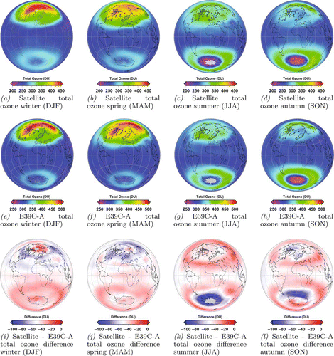
Seasonal mean values of total ozone derived from satellite instrument measurements and E39C-A are presented in figure 6. Please note that the colour bars are different for satellite and model data: since the E39C-A total ozone values have a positive bias (figure 5), we have done this to allow a better comparison of the two-dimensional patterns of the total ozone fields. The overall seasonal changes are well reproduced by the model. Particularly in the northern hemisphere (NH), the latitudinal structure compares in a reasonable way. For example, the position of the polar vortex during winter and spring, which is indicated by lower ozone values over Eurasia, is correctly simulated by E39C-A. While the northern hemisphere is dominated by a clear wavenumber 1 pattern, the distribution of ozone in the Southern Hemisphere (SH) has a much more zonally symmetric structure during all seasons which is also well captured by the model.

Figure 6. Seasonal mean values of total ozone (June 1995 to May 2008) from satellite instruments (top), the E39C-A simulation R2 (middle), and the difference between satellite measurements and model results (bottom).

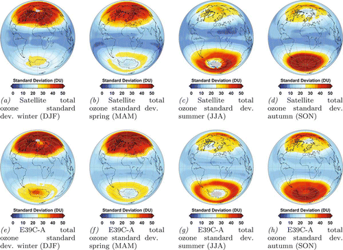
Another important diagnostic is the standard deviation. Figure 7 shows seasonal means of the standard deviation of total ozone, again for satellite data and model results. The overall seasonal change and the hemispheric patterns of the standard deviation in the model follows quite well the respective values from observations, but there are some differences in details, for example in the distribution of the standard deviation in northern winter (DJF) high latitudes. While in E39C-A, the variability is low in the centre of the polar vortex (approximately between northern Europe and the North Pole) and higher in the surroundings, the satellite data show high variability in the vortex centre and a lower standard deviation over North America and eastern Asia. This finding can be explained by the fact that the polar vortex is too stable in the model, i.e. that the number of minor and major warmings is lower than observed (e.g. Stenke et al. 2008). Note that the general higher standard deviation is also due to the absolute higher total ozone values in E39C-A compared to observations. In the summer hemisphere (SH, DJF) the standard deviation is much higher in the model, but the region of maximum variability agrees fairly well with those derived from observed values. Another clear difference is found in the SH spring time months (SON) indicating a weaker variability in the South Polar region. This is the result of a too cold polar lower stratosphere in E39C-A (‘cold pole problem’) reducing the dynamical variability in this region strongly.

Figure 7. Seasonal mean values of total ozone standard deviations (June 1995 to May 2008) from satellite instruments (top) and the E39C-A simulation R2 (bottom).

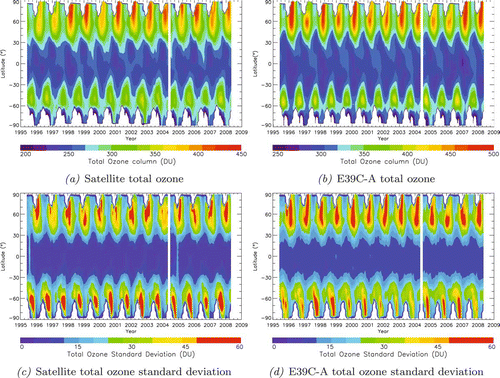
The evolution of the total ozone and standard deviation as a function of latitude and time for satellite measurements and model results is presented in figure 8. Note that the colour bars of the total ozone are different for satellite and model data (like in figure 6) to better compare the latitude-time patterns. The overall latitude and time variations are well reproduced by the model.

Figure 8. Latitudinal evolution of total ozone (top) and standard deviation (bottom) from June 1995 to May 2008. Satellite data on the left side (a, c) and E39C-A model on the right side (b, d). Satellite measurements from April 2004 are not available; the corresponding resampled model data is therefore also missing.

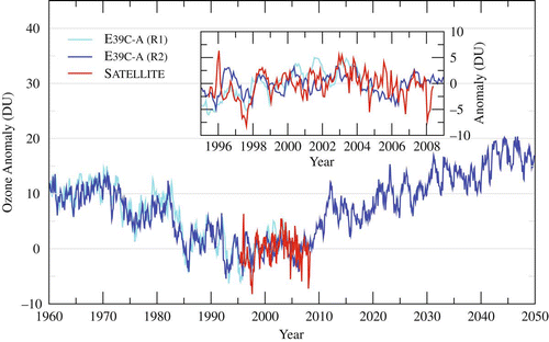
The results plotted in figure 9 should demonstrate how model data in combination with observations can be used to investigate short- and long-term changes. Here the temporal evolution of total ozone anomalies are presented for the near global mean, i.e. the average between 60° N and 60°S. The model values fit well with those from observations (see also Dameris et al. 2006) which is one hint that this model is suitable for future estimates. It is interesting to note that the decrease of total ozone after 2004 (which was the first year after maximum solar activity) was already predicted by the model 4 years ago (Dameris et al. 2006). In future, it will be interesting to watch if stratospheric ozone concentrations will significantly increase during the next decades as predicted by the model. Moreover, nearly all CCMs predict an accelerated recovery of the ozone layer (see Chapter 6 in World Meteorological Organization 2006) and even ‘ozone super-recovery’, i.e. the appearance of total ozone values higher than in the 1970's. The reason for this is the stratospheric cooling due to enhanced greenhouse gas concentrations which slows the rate of photochemical ozone destruction and hence leads to higher ozone concentrations in the extra-polar stratosphere. In contrast, ozone concentrations in the springtime polar lower stratosphere would decrease in response to cooling (not shown) because a cooling there would lead to more efficient chlorine activation on aerosol and polar stratospheric clouds and enhanced ozone destruction.

Figure 9. Total ozone anomalies over 60°N to 60°S. The mean annual cycle for 1995 to 2004 is subtracted from satellite measurements (red) and two E39C-A model simulations R1 from 1960 to 2004 (cyan) and R2 from 1960 to 2050 (blue). The inset shows a close-up for years where satellite measurements are available.

5. Conclusion

Global multi-year consistent data sets of atmospheric values and quantities are much needed to monitor changes within Earth's atmosphere. Drawing on the example of stratospheric ozone the paper has shown how data from different satellite instruments can be fitted together to produce a homogeneous dataset applicable not only for the analysis of short-term fluctuations but also for the study of long-term changes. A new technique for combining measurements derived from different space-borne instruments has been suggested. It allows us to compensate for drifts between sensors and is superior to other techniques, because it takes into account latitudinal and time dependent differences. We have demonstrated the ample possibilities of using such datasets for the validation of results derived from a three-dimensional atmospheric model system.

The combined use of long-term datasets derived from observations and complex atmospheric models systems is greatly required to further detect and understand changes in atmospheric composition and dynamics. The improvement of atmospheric models which are also used for prognostic studies is extremely important, because reliable assessments of future changes are needed to estimate consequences of natural and anthropogenic effects in a future atmosphere.

Acknowledgments

The authors would like to thank their colleagues P. Valks, W. Zimmer, and N. Hao working in the operational satellite retrieval system UPAS, to R. Spurr working on radiative transfer modelling and retrieval algorithms, and J-C. Lambert working on the geophysical validation. Thanks to ESA/DLR and EUMETSAT/DLR for providing the satellite data.

Appendix A: Ground Stations

Geographical position of all 79 selected ground stations are given in Table A1 for northern high and mid latitudes and in Table A2 for the tropics and southern hemisphere, respectively.

Table A1. Northern hemispheric mid and high latitude ground stations

WMO-Number	Instrument Type^a	Name	Latitude (°)	Longitude (°)	Elevation (m)	Country
NH High Latitude
315	B	Eureka	79.89	−85.93	10	Canada
89	D	Ny-Alesund	78.93	11.88	0	Norway
24	B	Resolute	74.72	−94.98	64	Canada
199	D	Barrow	71.32	−156.60	11	USA
262	B	Sodankyla	67.37	26.65	179	Finland
267	B	Sondrestrom	67.00	−50.98	150	Greenland
105	D	Fairbanks	64.80	−147.89	138	USA
284	B/D	Vindeln	64.25	19.77	0	Sweden
51	D	Reykjavik	64.13	−21.90	60	Iceland
123	B	Yakutsk	62.08	129.75	98	Russia
404	B	Jokioinen	60.80	23.50	103	Finland
43	D	Lerwick	60.15	−1.15	90	UK
NH Mid Latitude
165	D	Oslo	59.92	10.72	50	Norway
77	B	Churchill	58.75	−94.07	35	Canada
279	B	Norrkoping	58.58	16.12	0	Sweden
116	D	Moscow	55.75	37.57	187	Russia
309	B	Copenhagen	55.72	12.57	30	Denmark
21	B	Edmonton	53.57	−113.52	668	Canada
76	B	Goose Bay	53.32	−60.38	44	Canada
50	B/D	Potsdam	52.38	13.05	89	Germany
174	B	Lindenberg	52.22	14.12	98	Germany
241	B	Saskatoon	52.10	−105.28	550	Canada
316	B	DeBilt	52.00	5.18	0	Netherlands
318	B	Valentia	51.93	−10.25	0	Irland
68	D	Belsk	51.83	20.78	180	Poland
53	B/D	Uccle	50.80	4.35	100	Belgium
36	D	Camborne	50.22	−5.32	88	UK
338	B	Regina	50.21	−104.67	0	Canada
96	B/D	Hradec-Kralove	50.18	15.83	285	Czech-Republic
320	B	Winnipeg	49.91	−97.24	0	Canada
331	B	Poprad-Ganovce	49.03	20.32	0	Slovakia
290	B	Saturna	48.78	−123.13	0	Canada
99	B/D	Hohenpeissenberg	47.80	11.02	975	Germany
100	B/D	Budapest	47.43	19.18	140	Hungary
20	D	Caribou	46.87	−68.02	192	USA
35	B/D	Arosa	46.77	9.67	1860	Switzerland
19	D	Bismarck	46.77	−100.75	511	USA
301	B	Ispra	45.80	8.63	0	Italy
319	B	Montreal	45.47	−73.75	0	Canada
321	B	Halifax	44.90	−63.50	0	Canada
326	B	Longfenshan	44.75	127.60	0	China
226	D	Bucharest	44.48	26.13	92	Romania
201	D	Sestola	44.22	10.77	1030	Italy
40	D	Haute-Province	43.92	5.75	580	France
65	B	Toronto	43.78	−79.47	198	Canada
282	B	Kislovodsk	43.73	42.66	2070	Russia
12	D	Sapporo	43.05	141.33	19	Japan
305	B	Rome-University	41.90	12.52	0	Italy
261	B	Thessaloniki	40.52	22.97	4	Greece
308	B	Mardid	40.45	−3.55	0	Spain
67	D	Boulder	40.02	−105.25	1634	USA
208	D	Shiangher	39.77	117.00	13	China
82	B/D	Lisbon	38.77	−9.13	105	Portugal
293	D	Athens	38.00	23.70	15	Greece
346	B	Murcia	38.00	−1.17	69	Spain
107	D	Wallops-Island	37.87	−75.52	4	USA
252	D	Seoul	37.57	126.95	84	Korea
213	B/D	El-Arenosillo	37.10	−6.73	41	Spain
341	D	Hanford	36.32	−119.63	73	USA
106	D	Nashville	36.25	−86.57	182	USA
295	B	Mt. Waliguan	36.17	100.53	3816	China
14	D	Tateno	36.05	140.13	31	Japan
332	B	Pohang	36.03	129.38	0	Korea
13	D	Srinagar	34.08	74.83	1586	India
287	B	Funchal	32.65	−17.05	59	Portugal
7	D	Kagoshima	31.63	130.60	283	Japan
11	D	Quetta	30.18	66.95	1799	Pakistan
152	D	Cairo	30.08	31.28	35	Egypt
^a B: Brewer and D: Dobson

Table A2. Low latitude and southern hemispheric mid and high latitude ground stations

WMO- Number	Instrument Type^a	Name	Latitude (°)	Longitude (°)	Elevation (m)	Country
Low Latitudes^b (30°N –30°S)
10	B	New-Delhi	28.63	77.22	216	India
190	D	Naha	26.20	127.67	29	Japan
209	D	Kunming	25.02	102.68	1917	China
30	D	Marcus-Island	24.28	153.97	17	Japan
245	D	Aswan	23.97	32.45	193	Egypt
2	D	Tamanrasset	22.80	5.52	1395	Algeria
31	D	Mauna-Loa	19.53	−155.58	3397	USA
216	D	Bangkok	13.73	100.57	2	Thailand
322	B	Petaling-Jaya	3.10	101.65	46	Malaysia
214	D	Singapore	1.33	103.88	14	Singapore
175	D	Nairobi	−1.27	36.8	1710	Kenya
219	D	Natal	−5.83	−35.2	32	Brazil
84	D	Darwin	−12.47	130.83	0	Australia
191	D	Samoa	−14.25	−170.57	82	USA
200	D	Cachoeira-Paulista	−22.68	−45.00	573	Brazil
265	D	Irene	−25.25	28.22	1524	South-Africa
27	D	Brisbane	−27.47	153.03	5	Australia
340	D	Springbok	−29.67	17.90	1	South-Africa
SH Mid Latitude
343	D	Salto	−31.58	−57.95	31	Uruguay
159	D	Perth	−31.95	115.85	2	Australia
91	D	Buenos-Aires	−34.58	−58.48	25	Argentina
253	D	Melbourne	−37.48	144.58	125	Australia
92	D	Hobart	−42.88	147.33	4	Australia
256	D	Lauder	−45.03	169.68	3701	New-Zealand
342	D	Comodoro-Rivadavia	−45.78	−67.50	43	Argentina
29	D	Macquarie-Island	−54.48	158.97	6	Australia
339	D	Ushuaia	−54.85	−68.31	7	Argentina
SH High Latitude
232	D	Vernadsky-Faraday	−65.25	−64.27	7	Antarctica
101	D	Syowa	−69.00	39.58	21	Antarctica
57	D	Halley-Bay	−75.52	−26.73	31	Antarctica
268	D	Arrival-Heights	−77.83	166.40	250	Antarctica
314	B	Belgrano	−77.87	−34.63	255	Antarctica
111	D	Amundsen-Scott	−89.98	−24.80	2835	Antarctica
^aB: Brewer and D: Dobson
^b30°N – 30°S

References

- Aberle, B., Balzer, W., Von Bargen, A., Hegels, E., Loyola, D. and Spurr, R., 2002, GOME Level 0-to-1 algorithms description. Technical report, ER-TN-DLR-GO-022, Iss./Rev.5/B, http://earth.esrin.esa.it/pub/ESADOC/GOME/ .
- Balis, D., Koukouli, M., Loyola, D., Valks, P. and Hao, N., 2008, Validation of GOME-2 total ozone products (OTO/O3, NTO/O3) processed with GDP4.2. Technical report, SAF/O3M/AUTH/GOME-2VAL/RP/01, Revision 1B, http://www.wdc.dlr.de/sensors/gome2/SAF-O3M-AUTH-GOME-2VAL-RP-01.pdf
- Balis , D. , Kroon , M. , Koukouli , M. E. , Brinksma , E. J. , Labow , G. , Veefkind , J. P. and McPeters , R. D . 2007 . Validation of Ozone Monitoring Instrument total ozone column measurements using Brewer and Dobson spectrophotometer ground-based observations . Journal of Geophysical Research , 112 : D24546 doi:10.1029/2007JD008796
- Balis , D. , Lambert , J.- C. , van Roozendael , M. , Spurr , R. , Loyola , D. , Livschitz , Y. , Valks , P. , Amiridis , V. , Gerard , P. , Granville , J. and Zehner , C. 2007 . Ten years of GOME/ERS2 total ozone data. The new GOME data processor (GDP) version 4: 2. Ground-based validation and comparisons with TOMS V7/V8 . Journal of Geophysical Research , 112 : D07307 doi:10.1029/2005JD006376
- Bernhard , G. , Evans , R. D. , Labow , G. J. and Oltmans , S. J. 2005 . Bias in Dobson total ozone measurements at high latitudes due to approximations in calculations of ozone absorption coefficients and air mass . Journal of Geophysical Research , 110 : D10305 doi:10.1029/2004JD005559
- Bovensmann , H. , Burrows , J. P. , Buchwitz , M. , Frerick , J. , Noel , S. , Rozanov , V. V. , Chance , K. V. and Goede , A. P.H . 1999 . SCIAMACHY: Mission objectives and measurement modes . Journal of Atmospheric Science , 56 : 127 – 150 .
- Bramstedt , K. , Gleason , J. , Loyola , D. , Thomas , W. , Bracher , A. , Weber , M. and Burrows , J. P. 2003 . Comparison of total ozone from the satellite instruments GOME and TOMS with measurements from the Dobson network 1996–2000 . Atmospheric Chemistry and Physics , 3 : 1409 – 1419 .
- Burrows , J. P. , Weber , M. , Buchwitz , M. , Rozanov , V. V. , Ladstädter-Weissenmayer , A. , Richter , A. , de Beek , R. , Hoogen , R. , Bramstedt , K. , Eichmann , K.-U. , Eisinger , M. and Perner , D. 1999 . The Global Ozone Monitoring Experiment (GOME): Mission concept and first scientific results . Journal of Atmospheric Science , 56 : 151 – 175 .
- Callies , J. , Corpaccioli , E. , Eisinger , M. , Hahne , A. and Lefebvre , A . 2000 . GOME-2 – Metop's second generation sensor for operational ozone monitoring . ESA Bulletin , 102 : 28 – 36 .
- Chubachi , S. 3–7 September 1984 1985 . “ A special ozone observation at Syowa station, Antarctica from February 1982 to January 1983 ” . In Proceedings of the Quadrennial Ozone Symposium Edited by: Zerefos , C. S. and Ghazi , A. M. 3–7 September 1984 , 285 – 289 . Halkidiki, , Greece
- Cortesi , U. , Lambert , J. C. , de Clercq , C. , Bianchini , G. , Blumenstock , T. , Bracher , A. , Castelli , E. , Catoire , V. , Chance , K. V. , de Mazire , M. , Demoulin , P. , Godin-Beekmann , S. , Jones , N. , Jucks , K. , Keim , C. , Kerzenmacher , T. , Kuellmann , H. , Kuttippurath , J. , Iarlori , M. , Liu , G. Y. , Liu , Y. , McDermid , I. S. , Meijer , Y. J. , Mencaraglia , F. , Mikuteit , S. , Oelhaf , H. , Piccolo , C. , Pirre , M. , Raspollini , P. , Ravegnani , F. , Reburn , W. J. , Redaelli , G. , Remedios , J. J. , Sembhi , H. , Smale , D. , Steck , T. , Taddei , A. , Varotsos , C. , Vigouroux , C. , Waterfall , A. , Wetzel , G. and Wood , S. 2007 . Geophysical validation of MIPAS-ENVISAT operational ozone data . Atmospheric Chemistry and Physics , 7 : 4807 – 4867 .
- Dameris , M. , Grewe , V. , Ponater , M. , Eyring , V. , Mager , F. , Matthes , S. , Schnadt , C. , Stenke , A. , Steil , B. , Brühl , C. and Giorgetta , M. 2005 . Long-term changes in a transient simulation employing an interactively coupled chemistry-climate model under realistic forcings . Atmospheric Chemistry and Physics , 5 : 2121 – 2145 .
- Dameris , M. , Matthes , S. , Deckert , R. , Grewe , V. and Ponater , M . 2006 . Solar cycle effect delays onset of ozone recovery . Geophysical Research Letters , 33 L03 806-1-L03 806-4 doi:10.1029/2005GL024741
- Eyring , V. , Butchart , N. , Waugh , D. W. , Akiyoshi , H. , Austin , J. , Bekki , S. , Bodeker , G. , Boville , B. , Brühl , C. , Chipperfield , M. , Cordero , E. , Dameris , M. , Deushi , M. , Fioletov , V. , Frith , S. , Garcia , R. , Gettelman , A. , Giorgetta , M. , Grewe , V. , Jourdain , L. , Kinnison , D. , Mancini , E. , Manzini , E. , Marchand , M. , Marsh , D. , Nagashima , T. , Newman , P. A. , Nielsen , J. E. , Pawson , S. , Pitari , G. , Plummer , D. , Rozanov , E. , Schraner , M. , Shepherd , T. G. , Shibata , K. , Stolarski , R. , Struthers , H. , Tian , W. and Yoshiki , M . 2006 . Assessment of temperature, trace species, and ozone in chemistry-climate model simulations of the recent past . Journal of Geophysical Research , 111 : D22308 doi:10.1029/2006JD007327
- Eyring , V. , Waugh , D. W. , Bodeker , G. E. , Cordero , E. , Akiyoshi , H. , Austin , J. , Beagley , S. R. , Boville , B. , Braesicke , P. , Brühl , C. , Butchart , N. , Chipperfield , M. P. , Dameris , M. , Deckert , R. , Deushi , M. , Frith , S. M. , Garcia , R. R. , Gettelman , A. , Giorgetta , M. , Kinnison , D. E. , Mancini , E. , Manzini , E. , Marsh , D. R. , Matthes , S. , Nagashima , T. , Newman , P. A. , Nielsen , J. E. , Pawson , S. , Plummer , D. A. , Pitari , G. , Rozanov , E. , Schraner , M. , Scinocca , J. F. , Semeniuk , K. , Shepherd , T. G. , Shibata , K. , Steil , B. , Stolarski , R. , Tian , W. and Yoshiki , M. 2007 . Multi-model projections of stratospheric ozone in the 21st century . Journal of Geophysical Research , 112 : D16303 doi:10.1029/2006JD008332
- Farman , J. C. , Gardiner , B. G. and Shanklin , J. D. 1985 . Large losses of total ozone in Antarctica reveal seasonal ClOx/NOx interaction . Nature , 315 : 207 – 210 .
- Fioletov , V. , Kerr , J. , Hare , E. , Labow , G. and McPeters , R. 1999 . An assessment of the world ground-based total ozone network performance from the comparison with satellite data . Journal of Geophysical Research , 104 : 1737 – 1747 .
- Fischer , H. and Oelhaf , H. 1996 . Remote sensing of vertical profiles of atmospheric trace constituents with MIPAS limb-emission spectrometers . Applied Optics , 35 : 2787 – 2796 .
- Frith , S. , Stolarski , R. and Bhartia , P. K. 1–8 June 2004 2004 . “ Implications of version 8 TOMS and SBUV data for long-term trend ” . In Quadrennial Ozone Symposium Edited by: Zerefos , C. S. 1–8 June 2004 , 65 – 66 . Kos, , Greece
- Giorgetta , M. A. and Bengtsson , L. 1999 . Potential role of the quasi-biennial oscillation in the stratosphere-troposphere exchange as found in water vapor in general circulation model experiments . Journal of Geophysical Research , 104 : 6003 – 6019 .
- Gottwald , M. , Bovensmann , H. , Lichtenberg , G. , Noel , S. , von Bargen , A. , Slijkhuis , S. , Piters , A. , Hoogeveen , R. , von Savigny , C. , Buchwitz , M. , Kokhanovsky , A. , Richter , A. , Rozanov , A. Holzer-Popp, T , Bramstedt , K. , Lambert , J. C. , Skupin , J. , Wittrock , F. , Schrijver , H. and Burrows , J. B. 2006 . SCIAMACHY – Monitoring the changing earth's atmosphere , German Aerospace Center (DLR), Remote Sensing Institute (IMF) .
- Grewe , V. , Shindell , D. T. and Eyring , V. 2004 . The impact of horizontal transport on the chemical composition in the tropopause region: Lightning NOx and streamers . Advances in Space Research , 33 : 1058 – 1061 .
- Grewe , V. 2007 . Impact of climate variability on troposheric ozone . Science of the Total Environment , 374 : 167 – 181 .
- Hein , R. , Dameris , M. , Schnadt , C. , Land , C. , Grewe , V. , Köhler , I. , Ponater , M. , Sausen , R. , Steil , B. , Landgraf , J. and Brühl , C. 2001 . Results of an interactively coupled atmospheric chemistry-general circulation model: Comparison with observations . Annales Geophysicae , 19 : 435 – 457 .
- Johns , T. C. , Durman , C. F. , Banks , H. T. , Roberts , M. J. , McLaren , A. J. , Ridley , J. K. , Senior , C. A. , Williams , K. D. , Jones , A. , Rickard , G. J. , Cusack , S. , Ingram , W. J. , Crucifix , M. , Sexton , D. M.H. , Joshi , M. M. , Dong , B. , Spencer , H. , Hill , R. S.R. , Gregory , J. M. , Keen , A. B. , Pardaens , A. K. , Lowe , J. A. , Bodas-Salcedo , A. , Stark , S. and Searl , Y. 2006 . The New Hadley Centre Climate Model (HadGEM1): Evaluation of coupled simulations . Journal of Climate , 19 : 1327 – 1353 .
- Kerr , J. B. , Asbridge , I. A. and Evans , W. F.J . 1988 . Intercomparison of total ozone measured by the Brewer and Dobson spectrophotometers at Toronto . Journal of Geophysical Research , 93 : 11129 – 11140 .
- Koelemeijer , R. B. , Stammes , P. , Hovenier , J. W. and de Haan , J. F. 2001 . A fast method for retrieval of cloud parameters using oxygen A band measurements from the Global Ozone Monitoring Experiment . Journal of Geophysical Research , 106 : 3475 – 3490 .
- Kokhanovsky , A. A. , Rozanov , V. V. , Vountas , M. , Lotz , W. , Bovensmann , H. and Burrows , J. P. SCIAMACHY 1b to 2 OL Processing, Algorithm Theoretical Basis Document, Semi-Analytical CloUd Retrieval Algorithm for SCIAMACHY/ENVISAT . Technical report, ENVATB-IFE-SCIA-0003, Issue 2.0 . 2008 .
- Labow , G. J. , McPeters , R. D. and Bhartia , P. K. 1–8 June 2004 2004 . “ A comparison of TOMS, SBUV and SBUV/2 Version 8: Total column ozone data with data from ground stations ” . In Proceedings of the Quadrennial Ozone Symposium Edited by: Zerefos , C. S. 1–8 June 2004 , 123 – 124 . Kos, , Greece
- Lamago , D. , Dameris , M. , Schnadt , C. , Eyring , V. and Brühl , C. 2003 . Impact of large solar zenith angles on lower stratospheric dynamical and chemical processes in a coupled chemistry-climate model . Atmospheric Chemistry and Physics , 3 : 1981 – 1990 .
- Lambert , J.- C. , van Roozendael , M. , de Mazière , M. , Simon , P. C. , Pommereau , J. P. , Goutail , F. , Sarkissian , A. and Gleason , J. F. 1999 . Investigation of pole-to-pole performances of spaceborne atmospheric chemistry sensors with the NDSC . Journal of Atmospheric Science , 56 : 176 – 193 .
- Lambert , J. -C. , van Roozendael , M. , Simon , P. C. , Pommereau , J. P. , Goutail , F. , Gleason , J. F. , Andersen , S. B. , Arlander , D. W. , Bui Van , N. A. , Claude , H. , de la Noë , J. , de Mazière , M. , Dorokhov , V. , Eriksen , P. , Green , A. , Karlsen T⊘rnkvist , K. , Kåstad H⊘iskar , B. A. , Kyrö , E. , Leveau , J. , Merienne , M.- F. , Milinevsky , G. , Roscoe , H. K. , Sarkissian , A. , Shanklin , J. D. , Staehelini , J. , Wahlstr⊘m-Tellefsen , C. and Vaughan , G. 2000 . Combined characterization of GOME and TOMS total ozone measurements from space using ground-based observations from the NDSC . Advances in Space Research , 26 : 1931 – 1940 .
- Land , C. , Feichter , J. and Sausen , R. 2002 . Impact of vertical resolution on the transport of passive tracers in the ECHAM4 model . Tellus (B) , 54 : 344 – 360 .
- Lean , J. , Rottmann , G. , Kyle , H. , Woods , T. , Hickey , J. and Puga , L. 1997 . Detection and parameterisation of variations in solar mid- and near-ultraviolet radiation (22–400 nm) . Journal of Geophysical Research , 102 : 29 939 – 29 956 .
- Lerot , C. , van Roozendael , M. , van Geffen , J. , van Gent , J. , Fayt , C. , Spurr , R. , Lichtenberg , G. and von Bargen , M. 2009 . Six years of total ozone column measurements from SCIAMACHY nadir observations . Atmospheric Measurement Techniques , 2 : 87 – 98 .
- Levelt , P. E. , van den Oord , G. H.J. , Dobber , M. R. , Malkki , A. , Visser , H. , de Vries , J. , Stammes , P. , Lundell , J. O.V. and Saari , H. 2006 . The ozone monitoring instrument . IEEE Transactions on Geoscience and Remote Sensing , 44 : 1093 – 1101 .
- Loyola , D. G. . Cloud retrieval for SCIAMACHY . ERS-ENVISAT Symposium . Gothenburg, Sweden, 16–20 October.
- Loyola , D. G. . Automatic cloud analyses from polar-orbiting satellites using neural network and data fusion techniques . Proceedings of the IGARSS'04, Vol. IV, Anchorage/Alaska . Edited by: IEEE . 20 –24 August 2004 , pp. 2530 – 2533 .
- Loyola , D. G. , Thomas , W. , Livschitz , Y. , Ruppert , T. , Albert , P. and Hollmann , R. 2007 . Cloud properties derived from GOME/ERS-2 backscatter data for trace gas retrieval . IEEE Transactions on Geoscience and Remote Sensing , 45 : 2747 – 2758 .
- Mieruch , S. , Noel , S. , Bovensmann , H. and Burrows , J. P. 2008 . Analysis of global water vapour trends from satellite measurements in the visible spectral range . Atmospheric Chemistry and Physics , 8 : 491 – 504 .
- Miller , A. J. , Nagatani , R. M. , Flynn , L. E. , Kondragunta , S. , Beach , E. , Stolarski , R. , McPeters , R. D. , Bhartia , P. K. , Deland , M. T. , Jackman , C. H. , Wuebbles , D. J. , Patten , K. O. and Cebula , R. P. 2002 . A cohesive total ozone dataset from the SBUV(/2) satellite system . Journal of Geophysical Research , 107 : 4701 doi:10.1029/2001JD000853
- Rayner , N. A. , Parker , D. E. , Horton , E. B. , Folland , C. K. , Alexander , L. V. , Rowell , D. P. , Kent , E. C. and Kaplan , A. 2003 . Global analyses of sea surface temperatures, sea ice, and night marine air temperature since the late nineteenth century . Journal of Geophysical Research , 108 : 4407 doi:10.1029/2002JD002670
- Reithmeier , C. and Sausen , R. 2002 . ATTILA: Atmospheric Tracer Transport in a Lagrangian Model . Tellus (B) , 54 : 278 – 299 .
- Rex , M. , Salawitch , R. J. , Santee , M. L. , Waters , J. W. , Hoppel , K. and Bevilacqua , R. 2003 . On the unexplained stratospheric ozone losses during cold Arctic Januaries . Geophysical Research Letters , 30 doi:10.1029/2002GL016008
- Roeckner , E. , Arpe , K. , Bengtsson , L. , Christoph , M. , Claussen , M. , Dümenil , L. , Esch , M. , Giorgetta , M. , Schlese , U. and Schulzweida , U. ‘The atmospheric general circulation model ECHAM-4: Model description and simulation of present-day climate’ . Report No. 218, Max-Planck-Institut für Meteorologie, Hamburg . 1996 .
- Schnadt , C. , Dameris , M. , Ponater , M. , Hein , R. , Grewe , V. and Steil , B. 2002 . Interaction of atmospheric chemistry and climate and its impact on stratospheric ozone . Climate Dynamics , 17 : 501 – 517 .
- Slijkhuis, S., 1999, ENVISAT-1 SCIAMACHY Level 0 to 1c Processing, Algorithm Theoretical Basis Document. Technical report, ENV-ATB-DLR-SCIA-0041, Iss.1, http://earth.esa.int/services/sample_products/sciamachy/documentation/SCIAMACHY/ .
- Staehelin , J. , Kerr , J. , Evans , R. and Vanicek , K. Comparison of total ozone measurements of Dobson and Brewer spectrophotometers and recommended transfer functions . Technical report, TD N. 1147, No. 149, WMO . 2003 .
- Steil , B. , Dameris , M. , Brühl , C. , Crutzen , P. J. , Grewe , V. , Ponater , M. and Sausen , R. 1998 . Development of a chemistry module for GCMs: First results of a multiannual integration . Annales Geophysicae , 16 : 205 – 228 .
- Stenke , A. and Grewe , V. 2005 . Simulation of stratospheric water vapor trends: Impact on stratospheric ozone . Atmospheric Chemistry and Physics , 5 : 1257 – 1272 .
- Stenke , A. , Dameris , M. , Grewe , V. and Garny , H. 2008 . Implications of Lagrangian transport for coupled chemistry-climate simulations . Atmospheric Chemistry and Physics Discussion , 8 : 18727 – 18764 .
- Stolarski , R. S. and Frith , S. M. 2006 . Search for evidence of trend slow-down in the long-term TOMS/SBUV total ozone data record: the importance of instrument drift uncertainty . Atmospheric Chemistry and Physics , 6 : 4057 – 4065 .
- Stott , P. , Jones , G. , Lowe , J. , Thorne , P. , Durman , C. , Johns , T. and Thelen , J. 2006 . Transient climate simulations with the HadGem1 climate model: Causes of past warming and future climate change . Journal Climate , 19 : 2763 – 2782 .
- UNEP, 2006 ‘ Handbook for the Montreal Protocol on Substances that Deplete the Ozone Layer’ , Ozone Secretariat – United Nations Environment Programme, http://ozone.unep.org/Publications/MP_Handbook/index.shtml
- UNFCCC, 1998 ‘Kyoto Protocol to the United Nations Framework Convention on Climate Change’ http://unfccc.int/resource/docs/convkp/kpeng.pdf
- Valks, P. and Loyola, D., 2008, Algorithm theoretical basis document for GOME-2 total column products of ozone, minor trace gases, and cloud properties. Technical report, DLR/GOME-2/ATBD/01, Iss.1/C, http://www.wdc.dlr.de/sensors/gome2/DLR_GOME-2_ATBD_1C.pdf
- van Roozendael , M. , Peeters , P. , Roscoe , H. K. , De Backer , H. , Jones , A. , Vaughan , G. , Goutail , F. , Pommereau , J. P. , Kyrö , E. , Wahlstr⊘m , C. , Braathen , G. and Simon , P. C. 1998 . Validation of ground-based UV-visible measurements of total ozone by comparison with Dobson and Brewer spectrophotometers . Journal of Atmospheric Chemistry , 29 : 55 – 83 .
- van Roozendael , M. , Lambert , J. C. , Spurr , R. J.D. and Fayt , C. GOME direct fitting (GODFIT) GDOAS delta validation report . Technical Report, European Space Agency, Noordwijk, Netherlands, ERS exploitation AO/1–4235/02/I-LG . 2004 .
- van Roozendael , M. , Loyola , D. , Spurr , R. , Balis , D. , Lambert , J. C. , Livschitz , Y. , Valks , P. , Ruppert , T. , Kenter , P. , Fayt , C. and Zehner , C. 2006 . Ten years of GOME/ERS-2 total ozone data. The new GOME data processor (GDP) version 4: 1. Algorithm description . Journal of Geophysical Research , 111 doi:10.1029/2005JD006375
- Wang , P. , Stammes , P. , van der A , R. , Pinardi , G. and van Roozendael , M. 2008 . FRESCO+: an improved O2 A-band cloud retrieval algorithm for tropospheric trace gas retrievals . Atmospheric Chemistry and Physics Discussion , 8 : 6565 – 6576 .
- Weber , M. , Lamsal , L. N. , Coldewey-Egbers , M. , Bramstedt , K. and Burrows , J. P. 2005 . Pole-to-pole validation of GOME WFDOAS total ozone with ground-based data . Atmospheric Chemistry and Physics , 5 : 1341 – 1355 .
- West , D. H.D. 1979 . Updating mean and variance estimates: an improved method . Communications of the ACM , 22 : 532 – 535 .
- Williamson , D. L. and Rasch , P. J. 1994 . Water vapor transport in the NCAR CCM2 . Tellus (A) , 46 : 34 – 51 .
- World Meteorological Organization . ‘Scientific Assessment of Ozone Depletion: 1998’, WMO Global Ozone Research and Monitoring Project . Report No. 44 . 1998 .
- World Meteorological Organization . ‘Scientific Assessment of Ozone Depletion: 2002’, WMO Global Ozone Research and Monitoring Project . Report No. 47 . 2002 .
- World Meteorological Organization . ‘Scientific Assessment of Ozone Depletion: 2006’, WMO Global Ozone Research and Monitoring Project . Report No. 50 . 2006 .