Utilizing image texture to detect land-cover change in Mediterranean coastal wetlands

Abstract

Land-use/cover change dynamics were investigated in a Mediterranean coastal wetland. Change Vector Analysis (CVA) without and with image texture derived from the co-occurrence matrix and variogram were evaluated for detecting land-use/cover change. Three Landsat Thematic Mapper (TM) scenes recorded on July 1985, 1993 and 2005 were used, minimizing change detection error caused by seasonal differences. Images were geometrically, atmospherically and radiometrically corrected. CVA without and with texture measures were implemented and assessed using reference images generated by object-based supervised classification. These outputs were used for cross-classification to determine the ‘from–to’ change used to compare between techniques. The Landsat TM image bands together with the variogram yielded the most accurate change detection results, with Kappa statistics of 0.7619 and 0.7637 for the 1985–1993 and 1993–2005 image pairs, respectively.

1. Introduction

Land-cover change is an important feature of global environmental change (Dickinson 1995, Hall et al. 1995). Many of the world’s wetland systems are being converted to agricultural or urban use and this change can be monitored using remotely sensed data (Ringrose et al. 1988, Williams 1990, Mackey 1993, Markham et al. 1993, Jensen et al. 1995, Haack 1996) recorded at different times (Singh 1989). Each change detection method has its own merits and no method is optimal in all cases (Singh 1989, Mouat et al. 1993, Deer 1995, Coppin and Bauer 1996, Serpico and Bruzzone 1999). Examples include band differencing (Weismiller et al. 1977, Wink and King 2006), transformed band differencing (Nelson 1983), ratioing (Howarth and Wickware 1981), regression (Singh 1986), principal components analysis (PCA) (Byrne et al. 1980, Liu et al. 2004) and change vector analysis (CVA) (Malila 1980, Nackaerts et al. 2005). Support vector machine- (SVM-) based change detection also has great potential (Nemmour and Chibani 2006) as it uses structural risk minimization to solve two-class classification problems (Vapnik 1995).

CVA is particularly attractive as it can: (1) concurrently process and analyse change in all multi-spectral input data layers (as opposed to selected layers); (2) avoid compounding spatial-spectral errors inherent in multi-date classifications; (3) detect changes both in land cover and the condition of that land cover; and (4) separate the multidimensional change vector components of change images as it facilitates change interpretation and labelling (Johnson and Kasischke 1998).

Image texture is an important component of remotely sensed images. Texture refers to spatial variation in digital image spectral brightness (e.g. radiance, reflectance, digital number (DN)) and is due to spatial variation in one or a mix of the land surface, atmosphere or sensor field-of-view. Land-cover classes may have different textures in remotely sensed images and the similarity and differences between texture and spectral brightness have great potential for the classification of remotely sensed images (Lloyd et al. 2004, Berberoğlu et al. 2007).

The remote sensing of land cover can be complex in Mediterranean landscapes because: (1) the large temporal variance in the spectral properties of major land covers causes great within-class spectral variability; (2) the multiple spatial frequencies of landscape components result in complex scenes; and (3) the similar reflectance properties of some land covers make spectral separation difficult (e.g. light-toned, often calcareous, soils can have similar reflectance properties to urban areas and similar near-infrared reflectance to a crop canopy) (Berberoğlu 1999). As a result, the monitoring of land-cover change via remote sensing is difficult in Mediterranean regions. To minimize the impact of these problems, this paper evaluates an approach in which the CVA technique, using spectral data and texture measures (the grey level co-occurrence matrix (GLCM) and variogram), was used to estimate land-cover change in a Mediterranean coastal wetland.

2 Methods

2.1 Change vector analysis

CVA is a multivariate change detection technique that processes the full spectral and temporal dimensionality of image data and produces two outputs: change magnitude and change direction by geographical location. In addition, the capability to display some or all of the change information output from CVA relative to a background image has been found to be useful. CVA accepts as input n bands, transforms, or spectral features from each scene pair. These bands, therefore, comprise the axes of an n-dimensional space and the algorithm is robust to both the nature and number of these bands. Changed pixels should appear at two points in this measurement space, whereas unchanged pixels should appear at one point (figure 1).

Figure 1. Change vector in two-band radiometric space and the equation for Euclidean distance, D.

If change has occurred, the relationship between the two points can be characterized by a change vector with a measurable magnitude and direction (Johnson and Kasischke 1998) and this magnitude can be quantified using the Euclidean distance between the vector end-points. Direction angles can be measured for vectors for each pixel by trigonometry. Since vectors will be derived in polar coordinates, ϕ is measured from the y axis towards the x axis.

(1)

The many ways to quantify the magnitude and direction of change vary in complexity and thereby ease of implementation (Colwell et al. 1980).

2.2 Texture

Image texture can be derived from first-order measures (e.g. standard deviation) to more complicated measures (e.g. GLCM and variogram) and the utility of any particular measure for image classification can be evaluated using error matrices. In this study, texture was calculated on the first principal component of six wavebands (bands 1–5 and 7 of Landsat Thematic Mapper (TM)) for input to the CVA.

2.2.1 Grey level co-occurrence matrix

The GLCM measures the configuration of grey levels (i.e. brightness levels) in an image (Sonka et al. 1999) and has been applied in many remote sensing applications (Connors et al. 1984, Dreyer 1993, Augusteijn et al. 1995, Dikshit 1996, Bruzzone et al. 1997).

The GLCM comprises estimates of the transition probabilities (P) from grey level i to grey level j in two neighbouring pixels where neighbouring pixels are defined by a transition vector. For an image I (x,y) (i.e. the grey level set), and transition vector δ = (a,b)

(2)

The estimation is made by counting all occurrences of such transitions in the image and dividing by the number of pixels in the image. Thus, the GLCM can provide a statistical description of the relation between neighbouring pixels, which is an advantage over first-order statistics (Sali and Wolfson 1992). These matrices provide at least 14 textural features for the analysis of texture (Haralick et al. 1973). Four of these (contrast, angular second moment, dissimilarity, entropy) were found to be informative by Wood (1996) and so are used here.

1. Contrast:

   (3)

2. Angular second moment:

   (4)

3. Dissimilarity:

   (5)

4. Entropy:

   (6)

where i, j are the grey levels of paired pixels and P(i, j) are the probabilities of co-occurrence.

Computer code written in FORTRAN 77 was used to compute the GLCM and the four statistics (above) (hereafter called GLCM) on a per-pixel basis using 7×7 pixel windows. GLCM was computed for four directions: 0°, 45°, 90° and 135° clockwise from north and the statistics were derived from the average GLCM for all four directions.

2.2.2 Variogram

The variogram, the primary spatial descriptor in geostatistics, has been used to characterize spatial variability in remotely sensed imagery (Curran 1988, Ramsteın and Raffy 1989, Rubin 1990, Miranda and Carr 1994, Curran and Atkinson 1998, Berberoğlu et al. 2007). The variogram is a measure of the spatial dependence between pixel values, as it quantifies the dissimilarity of pixel values separated by a given vector (lag). The variogram is based on the postulate that pixels located further apart are less similar, or exhibit greater variance in their values, than pixels located closer together (Isaaks and Srivastava 1989, Goovaerts 1997). For continuous variables, such as reflectance in a given waveband, the experimental or sample variogram is computed for the p(h) paired sample points or observations; z(x_i), z(x_i + h). Half the expected squared difference between paired sample points of attribute z separated by lag h, z(x) and i = 1, 2, . . ., p(h) is calculated. For remotely sensed imagery the lag, h, is measured in units of one side of a pixel (Berberoğlu et al. 2000).

(7)

The sample variogram provides a set of discrete estimates of semi-variance at a set of discrete lags {h = 1, 2, . . ., [h]max} (Atkinson and Aplin 2004).

An algorithm based on the variogram computer code in the geostatistical software library GSLIB (Deutsch and Journel 1992) was used to estimate both the variogram at a lag of 1 unit (i.e. pixel) and variance for a moving window of 7×7 pixels. Mediterranean land-cover units can be small and discontinuous and object mixing limits the utility of large window sizes, hence this small window size (Berberoğlu et al. 2000). As the variogram at a lag of one pixel and variance are used together they will, for convenience, be referred to simply as the variogram measure of texture.

2.3 Accuracy assessment

Although many methods of accuracy assessment have been discussed in the remote sensing literature (Kalkhan et al. 1997, Koukoulas and Blackburn 2001), the most widely used method for assessing the accuracy of a classification is the error (or confusion) matrix (Foody 2001). As a simple cross-tabulation of the mapped class label against that observed on the ground or in reference data it provides an obvious foundation for accuracy assessment. The ‘traditional’ error matrix with Kappa coefficient has been used to assess change detection accuracy in multi-temporal comparison studies (Congalton 1991), where Kappa is the difference between the observed accuracy and the chance agreement divided by one minus that chance agreement (Lillesand and Kiefer 1994). In addition to Kappa, a test of significance was computed for each image pair to determine if an observed value of Kappa differed significantly from a hypothesized value (i.e. ‘null hypothesis’). When the probability of obtaining a Kappa value different to that in the null hypothesis is sufficiently low, then the difference is statistically significant (Goodman 1999).

3 Study area and data

3.1 Study area

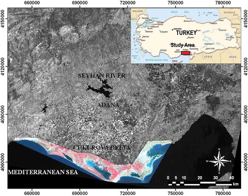
The study area is located on the southeastern Mediterranean coast of Turkey and is called Cukurova Deltas. It comprises three deltas formed by the rivers Seyhan, Ceyhan and Berdan and covers approximately 100 km by 15 km (figure 2). The land cover includes sand dunes, sand dune vegetation, agricultural land, salty plain, forest, wetland vegetation and water.

Figure 2. Location of study area in southern Turkey.

The land cover of the area is determined by agricultural, urban and tourism activities and their interaction with the local geology, soil, climate, hydrology and vegetation. These interactions are typical of this part of the Mediterranean coastal region and, as a result, this area makes an ideal environment in which to detect changes in Mediterranean coastal wetlands using remote sensing. These changes in land cover are complex. For example, agricultural fields reclaimed from coastal sand dunes are often abandoned after a few years of intensive use and this promotes further destruction. Extracted sand is laid routinely on agricultural fields as their salinity increases. Conversion from land to water is a consequence of coastal erosion, which may have resulted from decreased sediment supply following the construction of dams in the upper basin of the Seyhan River. Clearance of semi-natural vegetation due to grazing has resulted in seasonal changes, such as conversion to sand dunes and salty plains.

3.2 Dataset

The dataset comprised three Landsat TM images recorded on 7 July 1985, 27 July 1993 and 21 July 2005. The Mediterannean climate of the area is such that July is always warm and dry. Other data used for training and accuracy assessment included 1: 5000-scale State Hydraulics Department (DSI) maps and records of land cover for 1992; 1: 25 000-scale topographic maps; 57 class biotope maps for 1993 (Uzun et al. 1995) and 2005 (Altan et al. 2004, Akin 2007); various fine spatial resolution images, including 10 m spatial resolution Advanced Land Observing Satellite (ALOS)-Advanced Visible and Near Infrared Radiometer type 2 (AVNIR-2) imagery recorded in 2006; 4 m spatial resolution aerial photographs for various dates, including 1985, and field survey records and agricultural maps, together with expert knowledge.

4 Results

4.1 Pre-processing

Accurate image registration is essential for accurate change detection (Serra et al. 2003). The images were geometrically corrected and geocoded to the Universal Transverse Mercator (UTM) coordinate system using a reference image and 17 regularly distributed ground control points (GCPs) selected from the three Landsat TM images. Resampling used a nearest-neighbour algorithm (figure 3) and the transformation had root mean square errors (RMSE) of between 0.2 and 0.4 pixels, indicating that the images were located with an accuracy of less than a pixel.

Figure 3. Flow diagram of the methodology.

Spatial and temporal variation in the amount of dust in the atmosphere can mask real land-cover changes and suggest false land-cover changes. To help mitigate this problem, atmospheric correction, using an image-based COS(TZ) or COST method (Chavez 1996), was applied. This method uses the cosine of the solar zenith angle which, to a first order, is an approximation of atmospheric transmittance. It incorporates the elements of the dark object subtraction (DOS) method and assumes that any radiance received at the sensor from a dark object is due to atmospheric path radiance (Chavez 1996). The pixels containing the smallest brightness values were selected from the image and their value subtracted from the brightness values across the whole scene to reduce the influence of scattering (Serpico and Bruzzone 1999).

Following correction for geometry and scattering, the images were radiometrically normalized to each other. Various techniques have been developed for use in the Mediterranean region (Serrano et al. 2008) and the technique often used for this task is simple regression (Du et al. 2002). It is assumed that pixels sampled at time 2 are linearly related to pixels at the same locations at time 1. Pseudo-Invariant Features (PIFs), such as airports, rocks, deep-water bodies, permanent forest areas and large construction sites, were selected on the assumption that their reflectances are constant over time and the accuracy of this radiometric normalization was assessed using PCA. The procedure was applied to the three Landsat TM images and the linear correlation coefficients (r) for PIFs from two images were calculated both to provide a quality control metric to aid in the selection of PIFs and to assess the results of the normalization. If the linear correlation coefficient was less than 0.9, the area was deemed inappropriate as a PIF.

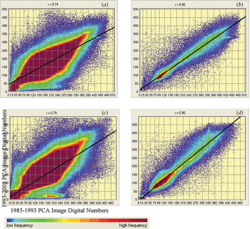
The correlation between the images was greater after atmospheric correction, indicating that atmospheric effects had been reduced. However, significant radiometric differences still existed between the images on each date due to the heterogeneous nature of the study area. Following radiometric normalization, r values increased from 0.74 to 0.96 and from 0.79 to 0.96 for the years between 1985 and 1993 and 1993 and 2005, respectively (figure 4).

Figure 4. (a), (c) Linear regression diagram for PCA of July 1985–1993 and 1993–2005. (b), (d) The same image pairs following radiometric normalization results using PIFs.

4.2 Creation of a reference dataset

The accuracy of change detection results using spectral data alone and together with image texture derived from the co-occurrence matrix and variogram results is estimated using a test area within the study site. Creation of the reference data involved object-based supervised classification of 1985, 1993 and 2005 Landsat TM data using the eCognition software. The land-cover classification maps of the test area were corrected manually using the dataset described in section 3.2. Field survey records and detailed biotope maps (Uzun et al. 1995, Altan et al. 2004, Akin 2007) coincided with image acquisitions in 1993 and 2005. In addition to this dataset, some expert knowledge was also utilized for the 1985 image classification. The object-based classification approach involved the integration of vector data and raster images within a geographical information system (GIS) and enabled the knowledge-free extraction of image object primitives at different spatial resolutions, a so-called multi-resolution segmentation. The segmentation operated as a heuristic optimization procedure which minimized the average heterogeneity of image objects at a given spatial resolution for the whole scene (Bian and Walsh 1992). The objective was to construct a hierarchical net of image objects, in which fine-scale objects were sub-objects of coarser objects. Due to the hierarchical structure, the image data were simultaneously represented at different spatial resolutions. The defined local object-orientated context information was then used together with other (spectral, form, texture) features of the image objects for classification. The next stage involved a supervised per-field classification with the nearest-neighbour algorithm and field boundary data generated as a result of image segmentation. Each field was assigned to one of seven land-cover classes: sand dunes, sand dune vegetation, agricultural, salty plain, forest, wetland vegetation and water. The classification results were corrected manually, using ground data from the biotope maps (Uzun et al. 1995, Altan et al. 2004), fine spatial resolution images and field survey records. The change analysis results were masked out from the reference data for the test area and then cross-tabulated in order to derive the ‘from–to’ change data needed to calculate ‘class-by-class’ change.

4.3 Change vector analysis

All texture measures were extracted from the first principal component of six wavebands (bands 1–5 and 7) of the Landsat TM images (figures 5 and 6) to create texture waveband(s), principal component transformation being one of the most widely used methods for compressing multiband data into one image (Benediktsson and Sveinsson 1997). Spectral and textural information were used separately and in combination within the CVA. A comparison study by Berberoğlu and Akin (2008) demonstrated that CVA was the most accurate change detection technique for this region in comparison with other traditional techniques. For this reason CVA was used within this study. Class-by-class texture information, including minimum, maximum and mean values, is given in tables 1 and 2.

Table 1. Mean values of GLCM for six land-cover classes and water.

Land-cover classes	GLCM
	1985				1993				2005
	a	b	c	d	a	b	c	d	a	b	c	d
Sand dunes	8.06	0.54	1.59	2.29	11.1	0.50	1.93	2.43	7.31	0.55	1.54	2.25
Sand dune vegetation	13.6	0.50	2.07	2.38	16.5	0.47	2.42	2.43	11.4	0.51	1.95	2.33
Agricultural	10.4	0.49	1.81	2.52	13.2	0.44	2.14	2.67	9.93	0.49	1.80	2.53
Salty plain	11.5	0.48	1.98	2.50	13.0	0.42	2.28	2.72	9.46	0.48	1.85	2.52
Forest	10.5	0.47	1.92	2.58	11.6	0.43	2.13	2.72	8.03	0.49	1.71	2.57
Wetland vegetation	8.35	0.62	1.49	1.99	7.56	0.62	1.39	1.96	4.49	0.67	1.07	1.81
Water	10.3	0.71	1.45	1.71	11.6	0.68	1.51	1.72	7.76	0.70	1.30	1.69

a, contrast; b, angular second moment; c, dissimilarity; d, entropy.

Table 2. Minimum, maximum and mean values of variogram for six land-cover classes and water.

Land cover classes	Variogram matrix
	1985			1993			2005
	Min	Max	Mean	Min	Max	Mean	Min	Max	Mean
Sand dunes	0.31	2171	105.2	0.71	2775	161.1	0.64	1771	129.3
Sand dune vegetation	3.41	1859	136.5	2.44	2114	174.5	2.49	1107	109.5
Agricultural	0.53	3994	90.6	0.78	5741	125.6	0.44	2974	107.6
Salty plain	0.31	3806	114.2	1.7	3777	198.6	0.93	1955	153.5
Forest	0.47	2048	120.7	1.12	3143	174.1	0.68	1894	119.0
Wetland vegetation	0.72	2230	251.5	1.84	2587	201.7	0.58	2261	169.2
Water	0.06	2976	88.03	0.17	3309	106.4	0.13	2180	85.01

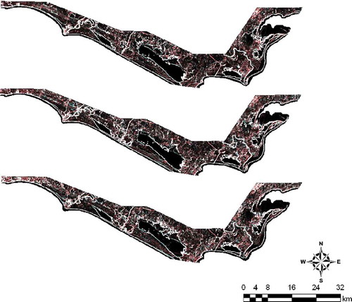
Figure 5. GLCM texture for 1985, 1993 and 2005 Landsat TM images.

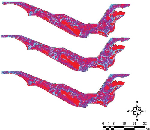
Figure 6. Variogram texture for 1985, 1993 and 2005 Landsat TM images.

The magnitude of change was computed using the spectral and textural information separately and together for: (1) the six bands of the Landsat TM images (spectral), (2) six bands of the Landsat TM images with GLCM output (spectral plus GLCM), (3) six bands of the Landsat TM images with variogram output (spectral plus variogram), (4) six bands of Landsat TM images with GLCM and variogram output together (complete).

A logarithmic transformation was applied to the resulting images to produce an approximately Gaussian distribution and the new mean and standard deviation values were used to determine a range of thresholds for change detection. Standard deviations of, 3σ, 2.5σ, 2σ, 1.8σ, 1.6σ, 1.5σ, 1.4σ were evaluated using the various types of ground data; 1.5σ was selected as providing the most realistic breakpoint in this dataset and the magnitude image reclassified. The value ‘0’ was assigned to no change areas and ‘1’ for changed areas and, as a result, a new image was created for each date. These change pixels were then masked out from the object-based classification result to prepare a change matrix. This matrix determined ‘from–to’ change and so enabled comparison of the accuracies achieved as a result of using different inputs to the CVA.

Evaluation of the two texture measures, GLCM and variogram, was based on change detection accuracy. Error matrices also provided information on confusion between classes. Total changed and unchanged pixels were used within the accuracy assessment. Change detection outputs resulting from different inputs were cross-tabulated against ground data for image pairs 1985–1993 and 1993–2005 (figure 7). Error matrices were used to assess the accuracy achieved both with and without the addition of texture (table 3).

Table 3. Comparison of change detection accuracy (Kappa) for four change detection procedures.

Dates	Spectral	GLCM	Variogram	Complete
1985–1993	0.5516	0.6681	0.7619	0.7409
1993–2005	0.58	0.6134	0.7637	0.7639

Figure 7. CVA outputs for the study area: spectral (a) 1985–1993, (e) 1993–2005; spectral with GLCM (b) 1985–1993, (f) 1993–2005; spectral with variogram (c) 1985–1993, (g) 1993–2005; spectral with variogram and GLCM (d) 1985–1993, (h) 1993–2005.

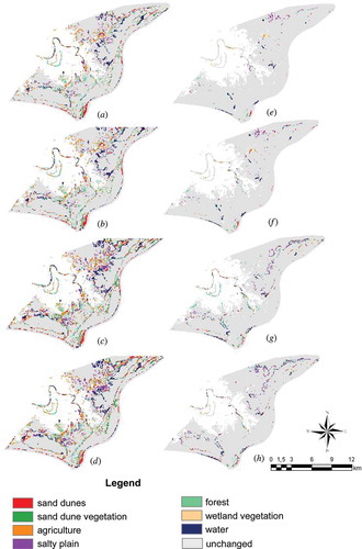
The largest change detection accuracy of 0.76 (i.e. 76%) was achieved using spectral data with the variogram texture measure for the 1985–1993 image pair. While the use of the GLCM in addition to the variogram did not increase the change detection accuracy for the 1985–1993 image pair, it did increase change detection accuracy slightly for the 1993–2005 image pair (figure 8). The GLCM and variogram overemphasized the field boundaries. In addition to boundaries, it also revealed useful information about the texture structures within land-cover classes.

Figure 8. Comparison of CVA results for spectral bands of Landsat TM data with and without variogram outputs.

Tests of significance yielded similar results to those of the Kappa analysis alone. Spectral data and variogram texture measures were correlated for both image pairs (tables 4 and 5). The significance values were 1.54 ×10⁻²³, indicating that the correlation is statistically significant.

Table 4. Test of significance results for 1985–1993 image pairs.

	Paired samples correlations (1985–1993)
		n	Correlation	Significance
Pair 1	ref & spect	212 083	0.75	0.00
Pair 2	ref & cooc	212 083	0.78	0.00
Pair 3	ref & semi-variogram	212 083	0.85	0.00
Pair 4	ref & complete	212 083	0.85	0.00

Table 5. Test of significance results for 1993–2005 image pairs.

	Paired samples correlations (1993–2005)
		n	Correlation	Significance
Pair 1	ref & spect	212 084	0.78	0.00
Pair 2	ref & cooc	212 084	0.81	0.00
Pair 3	ref & semi	212 084	0.88	0.00
Pair 4	ref & complete	212 084	0.88	0.00

Sig* 1.54×10⁻²³.

Table 6. Change in hectares defined using CVA with four change detection procedures and ground data.

	Spectral		GLCM		Variogram		Complete		Ground data
Land-cover classes	1985–1993	1993–2005	1985–1993	1993–2005	1985–1993	1993–2005	1985–1993	1993–2005	1985–1993	1993–2005
Sand dunes	239.49	22.05	266.22	41.4	380.88	74.61	381.15	71.28	495.9	411.84
Sand dune vegetation	107.19	3.42	105.75	5.67	162.09	16.11	162.18	15.84	307.71	153.36
Agricultural	472.41	31.05	496.62	39.06	675.99	46.17	676.17	44.37	1168.65	308.52
Salty plain	273.51	72.72	303.57	114.75	510.3	156.96	510.75	196.11	914.31	645.66
Forest	392.31	27	411.75	60.3	493.02	198.9	493.02	108.45	693.45	397.35
Wetland vegetation	46.26	6.21	52.29	12.42	75.87	57.51	75.96	37.98	140.94	106.02
Water	516.33	91.08	564.12	125.64	648.45	222.12	648.72	229.77	762.93	562.05
Unchanged	12212.82	14007.78	12060	13557.87	11313.72	13184.73	11312.37	13557.51	9777.43	11676.51

In addition to the error matrix and significance test, the area of change was calculated for each class and compared with ground data. The spatial distribution of the error for each method was mapped (figure 9). It was clear that the similar reflectance properties of sand dune vegetation and agriculture reduced change detection accuracy (figure 10).

Figure 9. Spatial distribution of error; spectral (a) 1985–1993, (e) 1993–2005; spectral with GLCM (b) 1985–1993, (f) 1993–2005; spectral with variogram (c) 1985–1993, (g) 1993–2005; spectral with GLCM and variogram (d) 1985–1993, (h) 1993–2005.

Figure 10. Mean spectral reflectance of major land-cover classes.

5 Discussion

For most land covers the spectral separation was subtle but the spatial patterns were distinct. For example, semi-natural vegetation comprises indistinct boundaries, whereas agricultural land cover is separated often by linear boundaries. Patches of semi-natural vegetation are so small that they typically form a distinctive texture (i.e. high frequency spatial variation) within regions as a whole. This fine spatial variation was captured by the variogram. As a result, change detection accuracy of sand dune vegetation and agriculture increased markedly with the addition of information from the variogram. However, GLCM statistics (except contrast), were not a useful discriminator for any individual classes.

Over 20 years, dramatic land-cover changes have occurred in these coastal wetlands. In the study area, approximately 906 ha of sand dunes, 460 ha of sand dune vegetation and 246 ha of wetland vegetation were converted primarily to agriculture and the total coverage of the seven land-cover classes decreased by 7061 ha (figure 11). Despite such a loss, these coastal dunes, with a length of over 100 km, cover an area of 9591 ha, which is the largest area of coastal dunes in Europe. Similar large land-cover changes have taken place in other parts of the Mediterranean Basin and have been detected using multi-temporal and multi-spectral satellite sensor data (Türker and San 2003, Zoran and Anderson 2006) and aerial photographs (Kadmon and Kremer 1999, D’Angelo et al. 2000). The majority of these studies utilized traditional techniques, such as image differencing and post-classification of spectral data using the standard band settings. Although this region has much spatial variability, the use of spatial information to discriminate between land covers in both space and time has not been utilized to date.

Figure 11. Change ratios for 1985–1993 and 1993–2005 for: (1) sand dunes, (2) sand dune vegetation, (3) agriculture, (4) salty plain, (5) forest, (6) wetland vegetation and (7) water.

Both measures of texture (GLCM and variogram) provided information that increased land-cover change detection accuracy over that for spectral data alone and this was true for both images pairs. The GLCM was used satisfactorily with spectral data to detect changes. However, incorporating the variogram resulted in the most accurate land-cover change detection with CVA. The addition of variogram texture information to the six bands of Landsat TM data increased by 21% and 18% the change detection accuracy compared with that achieved by spectral data alone. Changes within small and patchy land covers were detected accurately using just spectral data and the variogram. In particular, changes from sand dune vegetation and wetland vegetation to agriculture were detected in both image pairs. The land cover with a large area and continuous coverage, such as water and salty plains, was detected using all combinations (spectral, variogram and GLCM) with reasonable accuracy (table 6).

As a result of class mixing, spectral data and CVA alone resulted in low change detection accuracies for small land-cover parcels. The two texture measures emphasized class boundaries where the variance was large. Therefore, using the texture measures of the GLCM and variogram together did not result in any further increase in accuracy. The GLCM when used with spectral data for the large land-cover parcels (e.g. agricultural, water) also provided information on within-class variation. However, GLCM texture measures did not result in a significant increase in overall accuracy with either of the image pairs. This indicated that the variogram may provide useful additional information in a CVA for change detection in complex environments like the Mediterranean.

6 Conclusions

This paper aimed to assess the effectiveness of incorporating GLCM and variogram texture measures into CVA for change detection of a Mediterranean coastal wetland using multi-temporal remotely sensed data. Spectral and spatial information (in the form of various GLCM and variogram measures) were integrated with the aim of increasing the accuracy with which Landsat TM data and CVA could be used to detect Mediterranean coastal land-cover change. The textural information included the GLCM and variogram. The variogram texture measure (variogram at a lag of one pixel and variance), enabled more accurate change detection than using spectral data alone. Each texture measure increased the change detection accuracy for both image pairs. However, using the texture measures of the GLCM and variogram together did not result in further increases in accuracy. It is difficult to define a suitable texture measure to incorporate into the remote sensing of Mediterranean land-cover change. However, the following findings are important and provide some guidance for future research.

• Mediterranean land cover has considerable temporal and spatial variability, but relatively little spectral variability. Texture, as a measure of spatial variation, provided valuable information that enabled types of change to be quantified. GLCM and variogram texture measures resulted in an increase in accuracy for all classes over the use of Landsat TM spectral data alone.

• The accuracy of change detection using the GLCM and variogram depends on the size of objects in the image in relation to the spatial resolution of the imagery. Since the dominant land covers in an image are expected to occur in large parcels (e.g. fields), it may be anticipated that changes in these land covers can be detected most easily using texture information (i.e. GLCM and variogram).

• The variogram measure of texture provided greater change detection accuracy than the GLCM texture measures (angular second moment, contrast, dissimilarity and entropy) when used in combination with spectral data as an input to CVA.

• An advantage of the variogram over other texture measures is the capability to compute texture on a lag-by-lag basis. Only one lag could be analysed in this study due to the small and diverse land-cover objects, whereas generally the number of lags is limited only by the dimensions of the image. This was the main limitation to the use of the variogram for Landsat TM data in the Mediterranean environment. This limitation could be overcome using remotely sensed data with a finer spatial resolution.

• CVA was an effective approach as it can describe (1) change magnitude and (2) change direction. However, three disadvantages are the difficulty in identifying the change direction, the requirement for radiometric normalization and threshold selection.

This study reported the effectiveness and accuracy of using spectral data and texture (GLCM and variogram) for the remote sensing of Mediterranean land-cover change. This study has shown that the variogram is a promising tool and can be utilized for change detection. This novel approach can be applied to other delta and estuarine ecosystems in the Mediterranean where land-cover changes are rapid and pervasive.

References

- Akin, A., 2007, Assessing different remote sensing techniques to detect land use/cover changes in coastal zone of Cukurova Deltas. MSc thesis, Cukurova University Institution of Basic and Applied Sciences, Department of Landscape Architecture.
- Altan, T., Artar, M., Atik, M. and Cetinkaya, G., 2004, Cukurova Delta Biosphere Reserve Project. EU Life Third Countries TCY 99/TR/087 (Adana, Turkey: Cukurova University, Department of Landscape Architecture).
- Atkinson, P.M. and Aplin, P., 2004, Spatial variation in land cover and choice of spatial resolution for remote sensing. International Journal of Remote Sensing, 25, pp. 3687–3702.
- Augusteijn, M.F., Clemens, L.E. and Shaw, K.A., 1995, Performance evaluation of texture measures for ground cover identification in satellite images by means of a neural network classifier. IEEE Transactions on Geoscience and Remote Sensing, 33, pp. 616–625.
- Benediktsson, J.A. and Sveınsson, J.R., 1997, Feature extraction for multisource data classification with artificial neural networks. International Journal of Remote Sensing, 18, pp. 727–740.
- BerberoĞlu, S., 1999, Optimising the remote sensing of Mediterranean land cover. PhD thesis, Department of Geography, Faculty of Science, University of Southampton.
- BerberoĞlu, S. and Akin, A., 2008, Assessing different remote sensing techniques to detect land use/cover changes in the eastern Mediterranean. International Journal of Applied Earth Observation and Geoinformation, 11, pp. 46–53.
- BerberoĞlu, S., Curran, P.J., Lloyd, C.D. and Atkinson, P.M., 2007, Texture classification of Mediterranean land cover. International Journal of Applied Earth Observation and Geoinformation, 9, pp. 322–334.
- BerberoĞlu, S., Lloyd, C.D., Atkinson, P.M. and Curran, P.J., 2000, The integration of spectral and textural information using neural networks for land cover mapping in the Mediterranean. Computers and Geosciences, 26, pp. 385–396.
- Bian, L. and Walsh, S.J., 1992, Scale dependencies of vegetation and topography in a mountainous environment of Montana. Professional Geographer, 45, pp. 1–11.
- Bruzzone, L., Contese, C., Maselli, F. and Foli, F., 1997, Multisource classification of complex rural areas by statistical and neural-network approaches. Photogrammetric Engineering and Remote Sensing, 63, pp. 523–533.
- Byrne, G.F., Crapper, P.F. and Mayo, K.K., 1980, Monitoring land cover change by principal components analysis of multitemporal Landsat data. Remote Sensing of Environment, 10, pp. 175–184.
- Chavez, P.S., 1996, Image-based atmospheric corrections revisited and improved. Photogrammetric Engineering and Remote Sensing, 62, pp. 1025–1036.
- Colwell, J.E., Davis, G. and Thomson, F., 1980, Detection and Measurement of Changes in the Production and Quality of Renewable Resources. USDA Forest Service Final Report No. 145300-4-F (Ann Arbor, Michigan: ERIM).
- Congalton, R.G., 1991, A review of assessing the accuracy of classification of remotely sensed data. Remote Sensing of Environment, 37, pp. 35–46.
- Connors, R.W., Trivedi, M.M. and Harlow, C.A., 1984, Segmentation of a high resolution urban scene using texture operators. Computer Vision Graphics and Image Processing, 25, pp. 273–310.
- Coppin, P.R. and Bauer, M.E., 1996, Digital change detection in forest ecosystems with remote sensing imagery. Remote Sensing Reviews, 13, pp. 207–234.
- Curran, P.J., 1988, The semivariogram in remote sensing: an introduction. Remote Sensing of Environment, 24, pp. 493–507.
- Curran, P.J. and Atkinson, P.M., 1998, Geostatistics and remote sensing. Progress in Physical Geography, 22, pp. 61–78.
- D’Angelo, M., Enne, G., Madrau, S., Percich, L., Previtali, F., Pulina, G. and Zucca, C., 2000, Mitigating land degradation in Mediterranean agro-silvo-pastoral systems: a GIS-based approach. Catena, 40, pp. 37–49.
- Deer, P.J., 1995, Digital change detection techniques: civilian and military applications. In International Symposium on Spectral Sensing Research (Greenbelt, MD: Goddard Space Flight Center). Available online at: ltpwww.gsfc.nasa.gov/ISSSR-95/digitalc.htm
- Deutsch, C.V. and Journel, A.G., 1992, GSLIB: Geostatistical Software Library and User’s Guide (New York: Oxford University Press).
- Dickinson, R., 1995, Land processes in climate models. Remote Sensing of Environment, 51, pp. 27–38.
- Dikshit, O., 1996, Textural classification for ecological research using ATM images. International Journal of Remote Sensing, 17, pp. 887–915.
- Dreyer, P., 1993, Classification of land cover using optimised neural nets on SPOT data. Photogrammetric Engineering and Remote Sensing, 59, pp, 617–621.
- Du, Y., Teillet, P.M. and Cihlar, J., 2002, Radiometric normalization of multitemporal high-resolution satellite ımages with quality control for land cover change detection. Remote Sensing of Environment, 82, pp. 123–134.
- Foody, G.M., 2001, Accuracy of thematic maps derived from remote sensing. In Accuracy 2000: Proceedings of the 4th International Symposium on Spatial Accuracy Assessment in Natural Resources and Environmental Science, G.B.M. Heuvelink and M.J.P.M. Lemmens (Eds), pp. 217–224 (Delft, Holland: Delft University Press).
- Goodman, S., 1999, Toward evidence-based medical statistics. 1: The P value fallacy. Annals of International Medicine, 130, pp. 995–1004.
- Goovaerts, P., 1997, Geostatistics for Natural Resources Evaluation (New York: Oxford University Press).
- Haack, B., 1996, Monitoring wetland changes with remote sensing: an East African example. Environmental Management, 20, pp .411–419.
- Hall, C.A.S., Tian, H., Qi, Y., Pontius, G. and Cornell, J., 1995, Modeling spatial and temporal patterns of tropical land use change. Journal of Biogeography, 22, pp. 753–757.
- Haralick, R.M., Shanmugam, K. and Dinstein, I., 1973, Textural features for image classification. IEEE Transactions on Systems, Man, and Cybernetics, 3, pp. 610–621.
- Howarth, P.J. and Wickware, G.M., 1981, Procedures for change detection using Landsat. International Journal of Remote Sensing, 2, pp. 277–291.
- Isaaks, E.H. and Srivastava, R.M., 1989, An Introduction to Applied Geostatistics (New York: Oxford University Press).
- Jensen, J.R., Rutchey, K., Koch, M.S. and Narumalani, S., 1995, Inland wetland change detection in the Everglades Water Conservation Area 2A using a time series of normalised remotely sensed data. Photogrammetric Engineering and Remote Sensing, 61, pp. 199–209.
- Johnson, R.D. and Kasischke, E.S. 1998, Change Vector Analysis: A technique for the multispectral monitoring of land cover and condition. International Journal of Remote Sensing, 19, pp. 411–426.
- Kadmon, R. and Kremer, R.H., 1999, Studying long-term vegetation dynamics using digital processing of historical aerial photographs. Remote Sensing of Environment, 68, pp. 164–176.
- Kalkhan, M.A., Reich, R.M. and Czaplewski, R.L., 1997, Variogram estimates and confidence intervals for the Kappa measure of classification accuracy. Canadian Journal of Remote Sensing, 23, pp. 210–216.
- Koukoulas, S. and Blackburn, G.A., 2001, Introducing new ındices for accuracy evaluation of classified ımages representing semi-natural woodland environments, Photogrammetric Engineering and Remote Sensing, 67, pp. 499–510.
- Lillesand, T.M. and Kıefer, R.W., 1994, Remote Sensing and Image Interpretation (New York: Oxford University Press).
- Liu, Y., Nıshıyama, S. and Yano, T., 2004, Analysis of four change detection algorithms in bi-temporal space with a case study. International Journal of Remote Sensing, 25, pp. 2121–2139.
- Lloyd, C.D., BerberoĞlu, S., Atkinson, P.M. and Curran, P.J., 2004, A comparison of texture measures for the per-field classification of Mediterranean land cover International Journal of Remote Sensing, 25, pp. 3943–3965.
- Mackey, H.E., 1993, Six years of monitoring annual changes in a fresh water marsh with SPOT HRV data. In Looking to the Future With an Eye on the Past, Vol. 2, A.J. Lewis, pp. 222–229 (Bethesda: American Society for Photogrammetry and Remote Sensing and American Congress on Surveying and Mapping).
- Malila, W.A., 1980, Change Vector Analysis: An approach for detecting forest changes with Landsat. In Proceedings, Machine Processing of Remotely Sensed Data Symposium, Purdue University, West Lafayette, Indiana, pp. 326–335 ( Ann Arbor, MA: ERIM).
- Markham, A., Dudley, N. and Stolton, S., 1993, Some Like it Hot: Climate Change, Biodiversity and the Survival of Species (Gland: WWF International).
- Miranda, F.P. and Carr, J.R., 1994, Application of the semivariogram textural classifier (STC) for vegetation discrimination using SIR-B data of the Guiana Shield, north-western Brazil. Remote Sensing Reviews, 10, pp. 155–168.
- Mouat, D.A., Mahin, G.C. and Lancaster, J.S., 1993, Remote sensing techniques in the analysis of change detection. Geocarto International, 2, pp. 39–50.
- Nackaerts, K., Vaesen, K., Muys, B. and Coppin, P., 2005, Comparative performance of a modified change vector analysis in forest change detection. International Journal of Remote Sensing, 26, pp. 839–852.
- Nelson, R.F., 1983, Detecting forest canopy change due to insect activity using Landsat MSS. Photogrammetric Engineering and Remote Sensing, 49, pp. 1303–1314.
- Nemmour, H. and Chibani, Y., 2006, Multiple support vector machines for land cover change detection: An application for mapping urban extensions, Photogrammetric Engineering and Remote Sensing, 61, pp. 125–133.
- Ramstein, G. and Raffy, M., 1989, Analysis of the structure of radiometric remotely-sensed images. International Journal of Remote Sensing, 10, pp. 1049–1073.
- Ringrose, S., Matheson, W. and Boyle, T., 1988, Differentiation of ecological zones in the Okavango Delta, Botswana, by classification and contextual analyses of Landsat MSS data. Photogrammetric Engineering and Remote Sensing, 54, pp. 601–608.
- Rubin, T., 1990, Analysis of radar texture with variograms and other simplified descriptors. In Proceedings, Image Processing ′89, pp. 185–195 (Church Falls, VA: American Society for Photogrammetry and Remote Sensing).
- Sali, E. and Wolfson, H., 1992, Texture classification in aerial photographs and satellite. International Journal of Remote Sensing, 24, pp. 3311–3340.
- Serpico, S.B. and Bruzzone, L., 1999, Change detection. In Information Processing for Remote Sensing, C.H. Chen (Ed.), pp. 319–336 (Singapore: World Scientific Publishing).
- Serra, P., Pons, X. and Sauri, D., 2003, Post-classification change detection with data from different sensors: some accuracy considerations. International Journal of Remote Sensing, 24, pp. 3311–3340.
- Serrano, V.S.M., Cabello, F.P. and Lasanta, T., 2008, Assessment of radiometric correction techniques in analyzing vegetation variability and change using time series of Landsat images. Remote Sensing of Environment, 112, pp. 3916–3934.
- Singh, A., 1986, Change detection in the tropical forest environment of northeastern India using Landsat. In Remote Sensing and Tropical Land Management, M.J. Eden and J.T. Parry, pp 237–254 (New York: J. Wiley).
- Singh, A., 1989, Digital change detection techniques using remotely sensed data. International Journal of Remote Sensing, 10, pp. 989–1003.
- Sonka, M., Hlavac, V. and Boyle, R., 1999, Image Processing, Analysis and Machine Vision (London, UK: Chapman and Hall Computing).
- Türker, M. and San, B.T., 2003, SPOT HRV data analysis for detecting earthquake-induced changes in Izmit, Turkey. International Journal of Remote Sensing, 24, pp. 2439–2450.
- Uzun, G., Yucel, M., Yılmaz, K.T. and Berberoglu, S., 1995, Biotope Mapping in the Cukurova Deltas. Turkish Scientific and Technical Resarch Centre, Nr. TUBITAK- 17 TBAG.1164, Final Report (Adana, Turkey).
- Vapnik, V., 1995, The Nature of Statistical Learning Theory, 1st edn (New York: Springer Verlag), 2nd edn (Pacific Grove: PWS Publishing).
- Weismiller, R.A., Kristof, S.J., Scholz, D.K., Anuta, P.E. and Momin, S.A., 1977, Change detection in coastal zone environments. Photogrammetric Engineering and Remote Sensing, 43, pp. 1533–1539.
- Williams, M., 1990, Protection and retrospection. In Wetlands: A Threatened Landscape, M. Williams (Ed.), pp. 325–353 (Oxford: Blackwell).
- Wink, R. and King, D., 2006, Comparison of techniques for forest change mapping using Landsat data in Karnataka, India. Geocarto International, 21, pp. 49–57.
- Wood, J., 1996, The geomorphological characterisation of Digital Elevation Models. PhD thesis, University of Leicester, Leicester, UK.
- Zoran, M. and Anderson, E., 2006, The use of multi-temporal and multispectral satellite data for change detection analysis of the Romanian Black Sea coastal zone. Journal of Optoelectronics and Advanced Materials, 8, pp. 252–256.