Validating the MERIS Terrestrial Chlorophyll Index (MTCI) with ground chlorophyll content data at MERIS spatial resolution

Abstract

The Medium Resolution Imaging Spectrometer (MERIS) Terrestrial Chlorophyll Index (MTCI), a standard level 2 European Space Agency (ESA) product, provides information on the chlorophyll content of vegetation (amount of chlorophyll per unit area of ground). This is a combination of information on Leaf Area Index (LAI, area of leaves per unit area of ground) and the chlorophyll concentration of those leaves. The MTCI correlates strongly with chlorophyll content when using model, laboratory and field spectrometry data. However, MTCI calculated with MERIS data has only been correlated with surrogate chlorophyll content data. This is because of the logistical difficulties of determining the chlorophyll content of the area covered by a MERIS pixel (9 × 10⁴ m²). This paper reports the first attempt to determine the relationship between MTCI and chlorophyll content using actual MERIS data and actual chlorophyll content data.

During the summer of 2006 LAI and chlorophyll concentration data were collected for eight large (> 25 ha) fields around Dorchester in southern England. The fields contained six crops (beans, linseed, wheat, grass, oats and maize) at different stages of maturity and with different canopy structures, LAIs and chlorophyll concentrations. A stratified sampling method was used in which each field contained sampling units in proportion to the spatial variability of the crop. Within each unit 25 random points were sampled. This approach captured the variability of the field and reduced the potential bias introduced by the planting pattern or later agricultural treatments (e.g. pesticides or herbicides). At each random point LAI was estimated using an LAI-2000 plant canopy analyser and chlorophyll concentration was estimated using a Minolta-SPAD chlorophyll meter. In addition, for each field a calibration set of 30 contiguous SPAD measurements and associated leaf samples were collected.

The relationship between MTCI and chlorophyll content was positive. The coefficient of determination (R²) was 0.62, root mean square error (RMSE) was 244 g per MERIS pixel and accuracy of estimation (in relation to the mean) was 65%. However, one field included a high proportion of seed heads, which artificially increased the measured LAI and thus chlorophyll content. Removal of this field from the dataset resulted in a stronger relationship between MTCI and chlorophyll content with an R² of 0.8, an RMSE of 192 g per MERIS pixel and accuracy of estimation (in relation to the mean) of 71%.

1. Introduction

Remote sensing techniques offer a means of monitoring and evaluating terrestrial vegetation at a wide range of spatial and temporal scales (Running et al. 1995, Stow et al. 2004, Boyd and Danson 2005). However, the type of remotely sensed data required depends on the ecological questions being asked (Curran 2001). The three levels of questions are: what is the vegetation there? How much vegetation is there? And what is the condition of that vegetation? The first two questions can usually be answered using broadband remotely sensed data, whereas the third question usually requires data in narrow wavebands. Specifically, remotely sensed data recorded in narrow visible/near-visible wavebands can be used to estimate foliar biochemical content at local to global scales (Banninger 1991, Curran et al. 1997, Blackburn 2007). This information can, in turn, be used to quantify, understand and support the management of vegetated environments.

Chlorophyll is one of the more important foliar biochemicals and the content within a vegetation canopy is related positively to both the productivity of that vegetation and the depth and width of the chlorophyll absorption feature in reflectance spectra (Horler et al. 1983, Miller et al. 1991, Carter 1993, Broge and Leblanc 2001). Usually, the long wavelength (red) edge of this absorption feature moves to even longer wavelengths with an increase in chlorophyll content (Curran et al. 1990, Filella and Peñuelas 1994, Munden et al. 1994). Unfortunately, the position of this red edge (REP) is not an accurate indicator of chlorophyll content at high chlorophyll levels, and statistical techniques for estimating the REP were designed for small volumes of continuous spectral data rather than the large volumes of discontinuous spectral data produced by current space-borne spectrometers. However, since 2004 the European Space Agency (ESA) have been producing an operational level 2 product that estimates the relative position of the red edge. This product employs data from the Medium Resolution Imaging Spectrometer (MERIS) sensor and is called the MERIS Terrestrial Chlorophyll Index (MTCI) (Dash and Curran 2004). The MTCI is very simple to calculate yet it is sensitive to all and, notably, high values of chlorophyll content (Dash and Curran 2004, España-Boquera et al. 2006, Rossini et al. 2007).

The MTCI, the only chlorophyll content product from any space agency, provides an indication of terrestrial vegetation condition and has been applied successfully in many regional to global scale applications (Dash and Curran 2006, Curran et al. 2007, Lyalko et al. 2006). However, it has not yet been ‘validated’ using actual ground data on chlorophyll content and actual MERIS data.

Chlorophyll content of vegetation is a function of both the biophysical variable of Leaf Area Index (LAI; area of leaves per unit area of ground) and the biochemical variable of chlorophyll concentration (usually measured as the amount of chlorophyll per unit weight of leaf). Therefore, estimation of chlorophyll content requires information on both LAI and chlorophyll content.

Remotely sensed data has been used to estimate the LAI from a number of sensors at fine to moderate spatial resolution (Chen et al. 1997, Knyazikhin et al. 1998). As a result a number of operational global LAI datasets were developed (Sellers et al. 1996, Deng 2006, Baret et al. 2007). Some major steps were taken for direct validation of LAI products from coarse-resolution satellite data (i.e. comparing LAI derived from remotely sensed data with in situ data) using core sites representing a range of vegetation types; for example, BigFoot (Running et al. 1999) and VALERI (Baret et al. 2007). These are coordinated by the Working group on Calibration and Validation (WGCV) within the Committee on Earth Observation Satellites (CEOS) to ensure consistency in validation methodology. These validation methods are generally two-step processes: first, a high spatial resolution LAI map of the ground site is produced using in situ data, and then this is aggregated using a statistical method to produce an LAI map at the same spatial resolution of the satellite product for direct comparison (Justice at al. 2000).

Sampling chlorophyll content at MERIS spatial resolution (300 m) poses four logistical difficulties: (i) chlorophyll content varies with vegetation type; (ii) it is difficult to obtain a relatively uniform vegetation cover for a suitably sized plot (> 25 ha); (iii) there is no tried and tested sampling strategy for estimating chlorophyll content at MERIS spatial resolution and (iv) chlorophyll content is not usually recorded at the international sites that are currently used for validating coarse spatial resolution remotely sensed products.

The objectives of this study were (i) to develop a suitable sampling strategy for estimating, on the ground, chlorophyll content at MERIS spatial resolution; (ii) to implement this sampling strategy within three days of a MERIS overpass; and (iii) then relate the estimated ground chlorophyll content with MTCI.

2. Study site

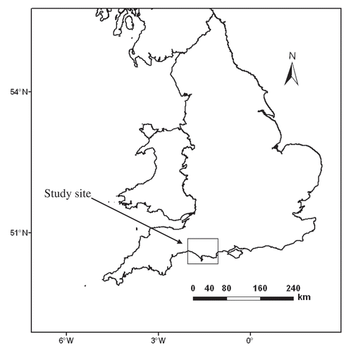
The study site is located near to Dorchester in Dorset, Southern England (latitude ≈ 50° 43′ N, longitude ≈ 02° 27′ W). The agricultural area in which it sits comprises suitably large (> 25 ha) and relatively flat fields of cropland including grassland (figure 1). The crops included beans, linseed, wheat, oats and maize.

Figure 1. Location of the study site in southern England.

2.1 Sampling field selection

The first stage was to select fields that represented, at the time of sampling, a wide range in chlorophyll content. Initially 18 fields were selected, but access problems restricted that number to eight (table 1). These fields contained six crops and were either a single large field or a contiguous block of similar fields, separated by a fence or thin hedge. Each crop was at different stage of maturity and had a different canopy structure, LAI and chlorophyll concentration, as is discussed below.

Table 1. Description of fields selected for sampling LAI and chlorophyll concentration.

Farm name	Crop	Area (ha)	Ordnance Survey sheet number	Code
Druce	Beans	51.6	SY79	Beans-I
Druce	Linseed	36.5	SY79	Linseed
West Down	Wheat	57.8	SY 89	Wheat
Finding	Grass	76.3	SY68	Grass-I
Finding	Grass	27.5	SY68	Grass-II
Baredown	Oats	42.0	SY89	Oats
Higher Alton	Maize	22.1	SY68	Maize
Deverel	Beans	31.0	SY79	Beans-II

2.1.1 Beans

The two fields covered a combined area of around 83 ha. The crop had a very weak directional orientation, leaves were numerous and greenness and LAI was clearly different between the two fields. There was a thin understorey and the presence of previous crops such as oil seed rape and sugar beat were evident. The total canopy height varied between approximately 40 and 120 cm (figure 2(a)).

Figure 2. Six of the fields selected for sampling: (a) beans, (b) linseed, (c) wheat, (d) grass, (e) oats and (f) maize.

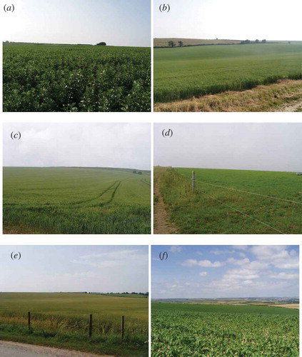
2.1.2 Linseed

This field covered an area of around 37 ha. The crop had some directional orientation and its small leaves were numerous and very green. There was a thin understorey and the presence of previous crops such as oil seed rape and sugar beat was evident. The total canopy height varied between approximately 20 and 60 cm (figure 2(b)).

2.1.3 Wheat

This field covered an area of around 58 ha. The crop had a strong directional orientation and leaves were long with some drooping at the leaf tip. There was no understorey but some variability in crop height and vigour. Generally, the ears were green but bright green leaves were prominent, suggesting a higher chlorophyll content than oats. The total canopy height varied between approximately 40 and 90 cm (figure 2(c)).

2.1.4 Grass

The two fields (Grass-I and Grass-II) covered a combined area of around 104 ha. There was no directional orientation and the small leaves formed a complex canopy over a well developed understorey. Both fields appeared similarly green, although the LAI was different. The total canopy height varied between approximately 10 and 60 cm (figure 2(d)).

2.1.5 Oats

This field covered an area of around 42 ha. The crop had a strong directional orientation, was at a late stage of maturity and had a high proportion seed heads. However, many leaves were still intact and so LAI was relatively high. There was a thin grass understorey and total canopy height varied between 30 and 80 cm (figure 2(e)).

2.1.6 Maize

This field covered an area of around 22 ha. Although smaller than the other fields, its square shape made it easy to sample. The crop had very strong directional orientation with wide gaps of between approximately 20 and 50 cm between rows. Leaves were large, numerous and very green and there was little or no understorey. The total canopy height varied between approximately 40 and 160 cm (figure 2(f)).

3. Sampling strategy

Collecting representative samples of both chlorophyll concentration and LAI to best represent the environment within a remotely sensed pixel has proved to be a challenging task (Cohen and Justice 1999, Tian et al. 2002, Wang et al. 2004, Gitelson et al. 2005, Baret et al. 2006, Yang et al. 2006). Methods can be classified into those that use the spatial autocorrelation within the area and those that do not.

The semivariogram-based method (Curran 1988) uses data acquired prior to sampling to calculate semivariograms. These are used to determine the spatial structure of the environment and thus the design of a sampling scheme (Tian et al. 2002). Unfortunately, it was not possible to apply this method as chlorophyll content varied rapidly with time. Therefore, a stratified sampling scheme was employed. Within each field between three to five sampling units (SU) were defined and within each SU 25 points were sampled along a transect (figure 3(a)). In the absence of major spatial variation the sampling units were distributed evenly across the field and in all cases the SU was no closer than 15 m from a field boundary.

Figure 3. Sampling strategy in each field (a) and sampling strategy within each sampling unit (b).

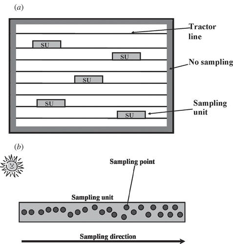
At each sampling point LAI and chlorophyll concentration were estimated and the GPS (global positioning system) location of the ends of the transect were noted. LAI estimates were undertaken from a tractor line nearest to the sun while facing the sun, although direct sunlight was shielded. Chlorophyll concentration estimates were made in the 10-cm diameter area from where LAI had been estimated. The distance between each consecutive measurement was random (figure 3(b)) and this helped to reduce bias introduced by the planting pattern or agricultural treatment (e.g. pesticides or herbicides). Each LAI estimate contrasted a single above the canopy measurement with at least four below the canopy measurements.

In situ estimates of LAI and chlorophyll concentration were undertaken between 11 and 19 July 2006.

3.1 LAI estimates

Crop canopy Leaf Area Index, (LAI; m² of leaves per m² of ground) was estimated using the LAI-2000 Plant Canopy Analyser (Li-Cor 1990). For logistical reasons LAI estimates were made throughout the day and under variable sky conditions. To prevent direct sunlight from illuminating the canopy and sun flecks from penetrating the canopy (both would result in an underestimation of LAI), all above and below canopy estimates were made under the shade of a large umbrella. This both reduced the illumination variability and ensured that the radiation was diffuse. A total of 25 independent estimates of LAI were made for each sampling unit in the field and each estimate integrated the area in which chlorophyll concentration was estimated.

3.2 Chlorophyll concentration estimates

Chlorophyll concentration was estimated instantaneously and non-destructively using a Minolta chlorophyll meter SPAD-502 (MINOLTA 2006). A calibration set of 30 simultaneous SPAD measurements and retained samples were collected for each of the six crop types. Retained leaf samples, each 96.78 mm² in area, were stored in DMF (N, N-dimethylformamide; analytical grade; Fisher Scientific, Loughborough, UK) in dark cool conditions for later analysis.

For a typical field the sampling intensity was as follows.

• Number of sampling units: 4

• Number of sampling points: 125

• Number of LAI estimates: 125 (each an average of 4–8 estimates)

• Number of chlorophyll concentration (SPAD) estimates: 125 (each an average of 6–8 measurements)

The leaf samples that had been stored in DMF were transferred to the laboratory for chlorophyll extraction. Each sample was diluted (1:3 with DMF) to produce a chlorophyll concentration that fell within the sensitive and linear range of the spectrophotometer. The mean of three replicate dilutions of each biological sample was used to represent the amount of chlorophyll a and chlorophyll b (μg ml⁻¹) within each sample. The spectrometer had 1–4 nm spectral resolution and specific absorption coefficients were used to estimate chlorophyll a and b in mg m⁻² (Wellburn 1994).

Estimated chlorophyll concentration for each crop was plotted against SPAD measurements made in the field. A second-order polynomial equation was used to describe the relationship between SPAD values and chlorophyll concentration (table 2). For each crop, chlorophyll concentration was correlated strongly with SPAD values: wheat having the strongest and grass having the weakest correlation. These relations were used to convert field SPAD measurements to chlorophyll concentration.

Table 2. SPAD calibration equations, where y represents chlorophyll concentration in mg m⁻² and x represents SPAD value.

Crop	Model equation	R^2
Beans	y = 0.073x^2 + 2.853x − 8.803	0.87
Linseed	y = 0.093x^2 + 0.088x + 47.1	0.95
Wheat	y = 0.118x^2 + 0.919x + 7.925	0.97
Grass	y = 0.019x^2 + 6.814x − 49.249	0.80
Oats	y = 0.122x^2 + 0.043x + 87.177	0.90
Maize	y = 0.091x^2 + 1.594x + 32.41	0.92

4. MERIS data processing

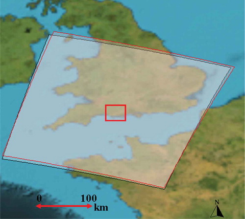
MERIS primary data products include calibrated instantaneous radiance estimates in each waveband at both full (300 m) and reduced (1200 m) spatial resolution. The secondary products include a number of geophysical and biophysical products over land, ocean and atmosphere. MERIS data are available at two levels of processing. Level 1 (L1) data are top-of-atmosphere radiances and level 2 (L2) data are atmospherically corrected top-of-canopy reflectance as well as geophysical and biophysical products. Two cloud-free MERIS L2 images for 15 and 18 July 2006 were selected as these were the closest in time to the dates of field sampling. Although sun-sensor geometry and atmospheric conditions can affect the radiances recoded by the instrument, the conditions were similar for the two images. Figure 4 shows the area covered by the MERIS scenes used in this study; as it can be seen, the study site lies at almost the same position in both scenes.

Figure 4. MERIS coverage. The black polygon represents the 15 July 2006 scene and the red polygon represents the 18 July 2006 scene. The rectangle in the centre represents the location of the study site.

Each MERIS scene was co-registered with high spatial resolution (20 m) Satellite Pour l’Observation de la Terre (SPOT) High Resolution Visible and Infrared (HRVIR)-2 scenes acquired on 24 July 2006 in order to increase the accuracy of MERIS georeferencing. This process was carried out by selecting ground control points which were identifiable both in SPOT and MERIS scenes. Individual fields were identified on the SPOT HRVIR-2 scenes and a vector boundary for each field was extracted by digitizing. These vectors were then overlain on the MERIS images. Number of MERIS pixels within each field boundary was variable. From each of these fields MERIS pixels which are more than half a pixel within the boundary of the field vector were selected for further analysis. This was based on the assumption that these pixels would provide a near similar spectral response for each field.

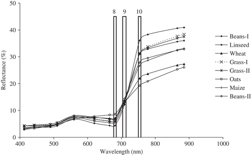
Figure 5 shows the spectral reflectance for each crop in 13 MERIS bands. For all crops there was high absorption in MERIS band 8 (centred at 681.25 nm), high reflectance in band 9 (centred at 708.75 nm) and an even higher reflectance in band 10 (centred at 753.75 nm). The first bean field, Beans-I, had the highest absorption in band 8 and highest reflectance in band 10, whereas Oats had the lowest absorption in band 8 and lowest reflectance in band 10. Both grass fields had a similar spectral reflectance but there was a large difference between the spectral reflectance of the two beans fields. This difference was because the second bean field, Beans-II, was recorded at a later date and was water stressed (sampling was within one of the hottest summer weeks) (Meteorological Office UK 2006).

Figure 5. Average spectral reflectance for each crop type in 13 MERIS wavebands overlain with the position of MERIS bands 8, 9 and 10.

5. Results

LAI, chlorophyll concentration and chlorophyll content were estimated for each SU. Where a MERIS pixel was wholly composed of a single canopy type and included a single SU then the average field measurements for that SU were applied to the MERIS pixel. Where more than one SU was present in a MERIS pixel the SUs were averaged. No account was made of the relative position of the SU in the MERIS pixel and no account was made of the MERIS point spread function.

5.1 Analysis of field data

Both LAI and chlorophyll concentration data obtained for each field are given in table 2. These show an average of 25 random measurements for each sampling unit and the standard deviation within each sampling unit for each field. Grass had the largest variation in LAI, because grass was partially grazed whereas other crops were managed. Linseed had largest variation in chlorophyll concentration; the unevenness of the field affected the water availability and in turn the crop growth.

5.1.1 Variation within each field

The variation in LAI and chlorophyll concentration within each field can be described using a normalized frequency distribution. This was determined by dividing the number of LAI and chlorophyll concentration estimates in each predefined range (LAI from 0 to 8 with an increment of 1, chlorophyll concentration from 0 to 700 with an increment of 50 mg m⁻²) by the total number of measurements in each field.

The LAI frequency distributions were symmetrical for all crops (figure 6(a)) except grass, where a large range in LAI was due to grazing. Among other crops Beans-I had the largest LAI (most SUs between 4 and 5) and Maize had the smallest LAI (most SUs between 1 and 2). This was because Beans-I was at the peak of its growing season whereas Maize was at the start of its growing season.

Figure 6. Normalized frequency distribution of LAI (a) and chlorophyll concentration (b) for each field.

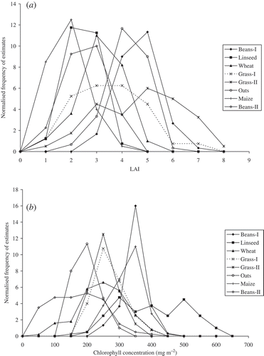
Unlike LAI, variations in chlorophyll concentration were large within each field, with the exception of Beans-I, Maize and grass (figure 6(b)). Linseed had a wide range of chlorophyll concentration (from 200 to 650 mg m⁻²) whereas Beans-I had a narrower range of chlorophyll concentration (from 300 to 400 mg m⁻²). Both grass fields had a similar range of chlorophyll concentration (200 to 400 mg m⁻²). Chlorophyll content was estimated for each sampling unit within each field by multiplying the average LAI by the average chlorophyll concentration for that sampling unit (table 3). Within sampling units the variation in chlorophyll content was greater than variation in chlorophyll concentration. This variation in chlorophyll content was resulted due to a variation in growth stage and crop type.

Table 3. Summary of (a) LAI, (b) chlorophyll concentration and (c) chlorophyll content for each sampling unit (SU) for all fields.

(a)
Crop type	No. of SU	LAI					Standard deviation
		SU1	SU2	SU3	SU4	SU5	SU1	SU2	SU3	SU4	SU5
Beans-I	3	4.0	3.8	4.7			0.7	0.8	0.5
Linseed	4	2.5	2.0	1.8	1.5		0.4	0.5	0.5	0.5
Wheat	5	2.9	2.2	2.7	2.8	2.7	0.9	0.7	0.7	0.7	1.0
Grass-I	4	4.0	2.9	3.5	1.7		0.9	1.3	1.3	0.7
Grass-II	4	4.3	3.0	5.1	4.4		1.4	1.3	1.6	1.6
Oats	3	3.7	3.3	4.1			0.7	0.7	0.7
Maize	4	1.5	1.6	0.9	1.7		0.6	0.6	0.6	0.8
Beans-II	4	2.4	1.1	2.5	2.3		0.8	0.4	0.7	0.6
(b)
		Chlorophyll concentration (mg m^−2)					Standard deviation (mg m^−2)
Crop type	No. of SU	SU1	SU2	SU3	SU4	SU5	SU1	SU2	SU3	SU4	SU5
Beans-I	3	313.5	325.0	314.3			33.7	21.5	40.6
Linseed	4	385.3	265.7	505.3	359.6		56.7	56.0	42.5	88.6
Wheat	5	211.9	223.8	276.9	223.0	166.7	71.7	68.8	53.9	44.5	71.8
Grass-I	4	225.7	267.4	232.4	256.7		37.4	54.7	44.5	39.5
Grass-II	4	244.2	221.2	242.0	219.9		44.8	33.1	31.7	37.0
Oats	3	183.6	158.6	178.8			34.2	32.9	41.0
Maize	4	307.5	323.4	317.9	246.5		33.8	34.7	37.8	40.9
Beans-II	4	173.2	54.2	208.5	164.9		63.8	26.8	68.9	55.0
(c)
		Chlorophyll content (g)
Crop type	No. of SU	SU1	SU2	SU3	SU4	SU5
Beans-I	3	12.44	12.45	14.78
Linseed	4	9.50	5.37	9.27	5.55
Wheat	5	6.10	4.84	7.49	6.20	4.46
Grass-I	4	8.96	7.78	8.04	4.27
Grass-II	4	10.38	6.57	12.26	9.73
Oats	3	6.87	5.23	7.31
Maize	4	4.50	5.11	2.86	4.10
Beans-II	4	4.16	0.59	5.23	3.81

5.1.2 Variation in the study site

For each field LAI, chlorophyll concentration and chlorophyll content was estimated as an average of all sampling units in that field. Figure 7 shows the LAI, chlorophyll concentration and chlorophyll content for each field along with the standard error (estimated from the standard deviation between all sampling units in a field). Maize had the smallest average LAI (∼1.4) and both Beans-I and Grass-II had the largest LAI (∼4.2) (figure 7(a)). Both grass fields had high variation in LAI between sampling units whereas Wheat had least variation in LAI between sampling units. Among all fields, Beans-II had the smallest average chlorophyll concentration (∼150 mg m⁻²) and Linseed had the largest average chlorophyll concentration (∼380 mg m⁻²) (figure 7(b)). Beans-I had the smallest and Linseed had the largest variation in chlorophyll concentration between sampling units. Beans-I had the largest chlorophyll content (∼13 g) and Beans-II had the smallest chlorophyll content (∼3.5 g) (figure 7(c)). Generally, variation in chlorophyll content between sampling units was larger than variation in LAI or chlorophyll concentration between sampling units.

Figure 7. Average values of (a) LAI; (b) chlorophyll concentration and (c) chlorophyll content for all fields used in this study. The error bar represents the standard error for sampling units in a field.

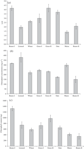
Differences between chlorophyll concentration and content were due to the manner in which they were derived. Chlorophyll concentration was derived from SPAD measurements. In order to compare field data with MERIS data, chlorophyll amount needed to be described as chlorophyll content (per surface area); this was achieved by the multiplication of chlorophyll concentration by LAI. Therefore, some crops with a similar chlorophyll concentration, e.g. Beans-I and Maize, had different chlorophyll content.

While in many cases LAI is directly related to chlorophyll content (Pinar and Curran 1996) there are specific circumstances where this is not the case, e.g. where there is not complete canopy closure and when a crop is ripening or is senescing. In the case of Beans-I and Maize these factors disassociated LAI from chlorophyll content.

5.2 Relationship between MTCI and chlorophyll content

For each field MTCI was estimated by averaging the MTCI values for the representative pixels. Per-field level average chlorophyll content was estimated as mg m⁻². Therefore, to get the chlorophyll content for an area equivalent to one MERIS pixel (9 × 10⁴ m²), the following expression was used:

(1)

where CC_MERIS is the chlorophyll content per MERIS pixel in g and CC_Field is the chlorophyll content per field in mg m⁻².

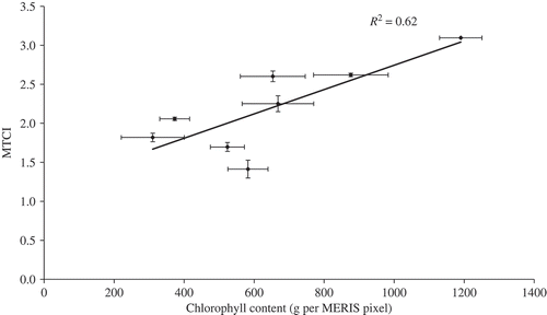
The coefficient of determination (R²) of 0.62 was statistically significant at 95% confidence level and, as can be seen in figure 8, the standard error of the MTCI estimates was low. Data for one field (Oats) was an outlier as it had been sampled at an early stage of maturity and so had many seed heads. These seed heads resulted in artificially high values of LAI and, as a consequence, chlorophyll content.

Figure 8. Relationship between MTCI and chlorophyll content for all fields.

6. Accuracy assessment

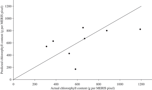
The accuracy in the relationship in figure 8 was assessed using the leave-one-out method (Lachenbruch and Mickey 1968) as the number of data points was low. This involved (i) removing one data point from the dataset; (ii) calculating a MTCI/chlorophyll content relationship for the remaining points; (iii) predicting chlorophyll content for the left-out data point; and (iv) repeating for all points (table 4). The root mean square error (RMSE) was used to compare predicted with actual chlorophyll content.

(2)

where CC_a is the actual chlorophyll content, CC_p is the predicted chlorophyll content using the leave-one-out method, and n is the number of fields (8).

Table 4. Predictive equations and coefficient of determination (R²) for the leave-one-out method, where y represents chlorophyll content in g and x represents MERIS MTCI value.

Field	Predictive equation	R^2
Beans-II	y = 357.4x − 108.19	0.61
Maize	y = 381.24x − 157.77	0.67
Wheat	y = 419.51x − 285.65	0.62
Oats	y = 544.9x − 600.19	0.80
Grass-I	y = 433.69x − 280.13	0.67
Linseed	y = 397.26x − 224.3	0.62
Grass-II	y = 382.42x − 201.51	0.58
Beans-I	y = 245.3x + 62.924	0.34

As shown in table 4, the coefficient of determination increased markedly when the Oats field was removed from the analysis (supporting the discussion in the previous section). Also when Beans-I was removed from the analysis the coefficient of determination decreased markedly as the high chlorophyll content in the field produced a large range in overall chlorophyll content.

Figure 9 shows the relationship between the actual and predicted chlorophyll content by the leave-one-out method. The RMSE was 244 g per MERIS pixel and the accuracy of estimation (in relation to the mean) was 65%.

Figure 9. Relationship between predicted and actual chlorophyll content using the leave-one-out method for all fields.

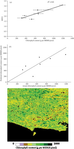
As the data point representing the Oats field was an outlier, it was removed from the data and the analysis was repeated using seven fields. The relationship between MTCI and chlorophyll content per MERIS pixel was stronger (R² = 0.8) (figure 10(a)). When the leave-one-out method was applied without the Oats field there was a decrease in RMSE to 190 g per MERIS pixel and this gave an accuracy of estimation (in relation to the mean) of 71% (figure 10(b)).

Figure 10. (a) Relationship between MTCI and chlorophyll content for all data except the oat field; (b) relationship between predicted and actual chlorophyll content using the leave-one-out method for all fields except the oat field; and (c) chlorophyll content map in g per MERIS pixel of the study site derived from the relationship between ground measurements and MTCI.

Therefore, a linear regression was used to establish the relationship between ground chlorophyll content and MTCI at MERIS spatial resolution. Based on this, chlorophyll content from MTCI can be derived as:

(3)

where chlorophyll content is expressed in g per MERIS pixel. This relationship was used to produce a chlorophyll content map of the study site (figure 10(c)).

7. Discussion

Accuracy assessment is essential for any biophysical product derived from satellite sensor data. In this experiment MTCI was correlated with chlorophyll content for a range of agricultural crops around Dorchester in southern England. The crops had different canopy structures and levels of maturity and this produced a wide range in chlorophyll content (345–1320 mg m⁻²). A stratified random sampling method was used to sample two key variables: LAI and chlorophyll concentration, which were combined to derive chlorophyll content. The MTCI for each field was obtained using two MERIS images acquired during the field campaign. Each MERIS image was co-registered with a finer spatial resolution SPOT HRV image to increase locational accuracy. Representative pixels were selected for each field and the average MTCI value was related to ground chlorophyll content. The relationship between MTCI and chlorophyll content was positive with a coefficient of determination (R²) of 0.62. Since the number of samples was low, a leave-one-out method was used to estimate accuracy. For eight fields the RMSE was 244 g per MERIS pixel and the accuracy of estimation (in relation to the mean) was 65%. One sample was an outlier; this had an inflated LAI and thus chlorophyll content as a result of seed heads in the canopy. Removal of this sample resulted in a stronger relationship between MTCI and chlorophyll content (R² = 0.8), a lower RMSE (192 g per MERIS pixel) and an increase in the accuracy of estimation (in relation to the mean 71%).

The two major sources of uncertainty were: (i) error in the field measurements and (ii) error in the laboratory analysis and, therefore, SPAD calibration, chlorophyll concentration and chlorophyll content.

8. Conclusion

Satellite remote sensing provides the opportunity to measure and monitor key photosynthetic pigments, such as chlorophyll content of vegetation canopies, which are a key and dynamic component of global ecosystems. The MTCI relates positively to chlorophyll content, notably to high values, and is being produced operationally by ESA. Given that the MTCI is the only available chlorophyll index from space-borne sensors there is now a real opportunity for systemic and reliable monitoring of vegetation function and condition. However, to understand fully the performance of the index and its utility in the provision of scientifically robust measures of canopy chlorophyll content (and concentration) there is a need to validate the index across a range of vegetative types and environmental conditions. The experiment provided a quantitative relationship between MTCI and ground chlorophyll content for a range of agricultural crops which aligns with model and greenhouse studies. Future work should aim in further refinement of this relationship using airborne sensor data, further MERIS data and a larger sample size.

Acknowledgement

We are grateful to ESA for providing funding under ESTEC Contract No. 19957/06/NL/EL and MERIS data and the local farmers for their help and support for this work. SPOT data were provided by ESA under a cat-1 project to JD.

References

- Banninger, C., 1991, Phenological changes in the red edge shift of Norway spruce needles and their relationship to needle chlorophyll content. Proceedings of the 5th International Colloquium—Physical Measurements and Signatures in Remote Sensing, 14–18 January 1991, Courcheval, France, pp. 155–158 ( Paris: ISPRS).
- Baret, F., Morissette, J.T., Fernandes, R.A., Champeaux, J.L., Myneni, R.B., Chen, J., Plummer, S., Weiss, M., Bacour, C., Garrigues, S. and Nickeson, J.E., 2006, Evaluation of the representativeness of networks of sites for the global validation and intercomparison of land biophysical products: Proposition of the CEOS-BELMANIP. IEEE Transactions on Geoscience and Remote Sensing, 44, pp. 1794–1803.
- Baret, F., Hagolle, O., Geiger, B., Bicheron, P., Miras, B., Huc, M., Berthelot, B., Nino, F., Weiss, M., Samain, O., Roujean, J.L. and Leroy, M., 2007, LAI, fAPAR and fCover CYCLOPES global products derived from VEGETATION: Part 1: Principles of the algorithm. Remote Sensing of Environment, 110, pp. 275–286.
- Blackburn, G.A., 2007, Hyperspectral remote sensing of plant pigments. Journal of Experimental Botany, 58, pp. 855–867.
- Boyd, D.S. and Danson, F.M., 2005, Satellite remote sensing of forest resources: three decades of research development. Progress in Physical Geography, 29, pp. 1–26.
- Broge, N.H. and Leblanc, E., 2001, Comparing prediction power and stability of broadband and hyperspectral vegetation indices for estimation of green leaf area index and canopy chlorophyll density. Remote Sensing of Environment, 76, pp. 156–172.
- Carter, G.A., 1993, Responses of leaf spectral reflectance to plant stress. American Journal of Botany, 80, pp. 239–243.
- Chen, J.M., Rich, P.M., Gower, S.T., Norman, J.M. and Plummer, S., 1997, Leaf area index of boreal forests: Theory, techniques and measurements. Journal of Geophysical Research, 102, pp. 29429–29443.
- Cohen, W.B. and Justice, C.O., 1999, Validating MODIS terrestrial ecology products: Linking in situ and satellite measurements. Remote Sensing of Environment, 70, pp. 1–3.
- Curran, P.J., 1988, The semivariogram in remote-sensing - An introduction. Remote Sensing of Environment, 24, pp. 493–507.
- Curran, P.J., 2001, Imaging spectrometry for ecological applications. International Journal of Applied Earth Observation and Geoinformation, 3, pp. 305–312.
- Curran, P.J., Dungan, J.L. and Gholz, H.L., 1990, Exploring the relationship between reflectance red edge and chlorophyll content in slash pine. Tree Physiology, 7, pp. 33–48.
- Curran, P.J., Kupiec, J.A. and Smith, G.M., 1997, Remote sensing the biochemical composition of a slash pine canopy. IEEE Transactions on Geoscience and Remote Sensing, 35, pp. 415–420.
- Curran, P.J., Dash, J. and Lllewellyn, G.M., 2007, Indian Ocean tsunami: The use of MERIS (MTCI) data to infer salt stress in coastal vegetation. International Journal of Remote Sensing, 28, pp. 729–735.
- Dash, J. and Curran, P.J., 2004, The MERIS Terrestrial Chlorophyll Index. International Journal of Remote Sensing, 25, pp. 5003–5013.
- Dash, J. and Curran, P.J., 2006, Relationship between herbicide concentration during the 1960s and 1970s and the contemporary MERIS Terrestrial Chlorophyll Index (MTCI) for southern Vietnam. International Journal of Geographical Information Science, 20, pp. 929–939.
- Deng, F., Chen, J.M., Plummer, S., Chen, M. and Pisek, J., 2006, Global LAI algorithm integrating the bidirectional information. IEEE Transactions in Geosciences and Remote Sensing, 44, pp. 2219–2229.
- España-Boquera, M.L., Cárdenas-Navarro, R., López-Pérez, L., Castellanos-Morales, V. and Lobit, P., 2006, Estimating the nitrogen concentration of strawberry plants from its spectral response. Communications in Soil Science and Plant Analysis, 37, pp. 2447–2459.
- Filella, I. and Peñuelas, J., 1994, The red edge position and shape as an indicator of plant chlorophyll content, biomass and hydric status. International Journal of Remote Sensing, 15, pp. 1459–1470.
- Gitelson, A., Vina, A., Ciganda, V., Rundquist, C. and Arkebauer, T., 2005, Remote estimation of canopy chlorophyll content in crops. Geophysical Research Letters, 32, pp. 1–4.
- Horler, D.N.H., Dockray, M. and Barber, J., 1983, The red edge of plant leaf reflectance. International Journal of Remote Sensing, 4, pp. 273–288.
- Justice, C., Belward, A., Morisette, J., Lewis, P., Privette, J. and Baret, F., 2000, Developments in the validation of satellite sensor products for the study of the land surface. International Journal of Remote Sensing, 21, pp. 3383–3390.
- Knyazikhin, Y., Martonchik, J.V., Myneni, R.B., Diner, D.J. and Running, S.W., 1998, Synergistic algorithm for estimating vegetation canopy leaf area index and fraction of absorbed photosynthetically active radiation from MODIS and MISR data. Journal of Geophysical Research, 103, pp. 32257–32275.
- Lachenbruch, P.A. and Mickey, M.R., 1968, Estimation of error rates in discriminant analysis. Technometrics, 10, pp. 1–11.
- Li-Cor, 1990, LAI-2000 Plant Canopy Analyzer Instruction Manual (Lincoln, NE, USA: LI-COR Biosciences).
- Lyalko, V.I., Shportyuk, Z.M., Sakhatskyi, O.L. and Sybirtseva, O.M., 2006, Land cover classification in Ukrainian carpathians using the MERIS Terrestrial Chlorophyl Index and red edge position from ENVISAT MERIS data. Kosmichna Nauka i Tekhnologiya, 12, pp. 10–14.
- Meterological Office UK, 2006, 2006—a year for the record books. Available online at: www.metoffice.gov.uk/corporate/pressoffice/2006/pr20061214.html ( accessed 25 June 2007).
- Miller, J.R., Wu, J., Boyer, M.G., Belanger, M. and Hare, E.W., 1991, Seasonal pattern in leaf reflectance red-edge characteristic. International Journal of Remote Sensing, 12, pp. 1509–1523.
- Minolta, 2006, Minolta SPAD 502 Meter, Spectrum Technologies. Available online at: www.specmeters.com/Chlorophyll_Meters/Minolta_SPAD_502_Meter.html ( accessed 25 June 2007).
- Munden, R., Curran, P.J. and Catt, J.A., 1994, The relationship between red edge and chlorophyll concentration in the Broadbalk winter wheat experiment at Rothamsted. International Journal of Remote Sensing, 15, pp. 705–709.
- Pinar, A. and Curran, P.J., 1996, Grass chlorophyll and the reflectance red edge. International Journal of Remote Sensing, 17, pp. 351–357.
- Rossini, M., Panigada, C., Meroni, M., Busetto, L., Castrovinci, R. and Colombo, R., 2007 Monitoraggio delle condizioni della farnia (Quercus robur L.) nel Parco del Ticino mediante tecniche di telerilevamento iperspettrale. Forest@, 4, pp. 194–203 [ in Italian].
- Running, S.W., Loveland, T.R., Pierce, L.L. and Nemani, R.R., 1995, A remote sensing based vegetation classification logic for global land cover analysis. Remote Sensing of Environment, 51, pp. 39–48.
- Running, S.W., Baldocchi, D., Turner, D.P., Gower, S.T., Bakwin, P.S. and Hibbard, K.A., 1999, A global terrestrial monitoring network integrating tower fluxes, flask sampling, ecosystem modelling and EOS satellite data. Remote Sensing of Environment, 70, pp. 108–127.
- Sellers, P.J., Los, S.O., Tucker, C.J., Justice, C.O., Dazlich, D.A., Collatz, G.J. and Randall, D.A.,1996, A revised land surface parameterization (SiB2) for atmospheric GCMS. Part II: The generation of global fields of terrestrial biophysical parameters from satellite data. Journal of Climate, 9, pp. 706–737.
- Stow, D.A., Hope, A., McGuire, D., Verbyla, D., Gamon, J., Huemmrich, F., Houston, S., Racine, C., Sturm, M., Tape, K., Hinzman, L., Yoshikawa, K., Tweedie, C., Noyle, B., Silapaswan, C., Douglas, D., Griffith, B., Jia, G., Epstein, H., Walker, D., Daeschner, S., Petersen, A., Zhou, L. and Myneni, R., 2004, Remote sensing of vegetation and land-cover change in Arctic tundra ecosystems. Remote Sensing of Environment, 89, pp. 281–308.
- Tian, Y.H., Woodcock, C.E., Wang, Y.J., Privette, J.L., Shabanov, N.V., Zhou, L.M., Zhang, Y., Buermann, W., Dong, J.R., Veikkanen, B., Hame, T., Andersson, K., Ozdogan, M., Knyazikhin, Y. and Myneni, R.B., 2002, Multiscale analysis and validation of the MODIS LAI product—I. Uncertainty assessment. Remote Sensing of Environment, 83, pp. 414–430.
- Wang, Y., Woodcock, C.E., Buermann, W., Stenberg, P., Voipioc, P., Smolanderc, H., Hame, T. Tiana, Y., Hua, J. Knyazikhin, Y. and Myneni, R.B., 2004, Evaluation of the MODIS LAI algorithm at a coniferous forest site in Finland. Remote Sensing of Environment, 91, pp. 114–127.
- Wellburn, A.R., 1994, The spectral determination of chlorophyll-a and chlorophhyll-b, as well as total carotenoids, using various solvents with spectrophotometers of different resolution. Journal of Plant Physiology, 144, pp. 307–313.
- Yang, W., Tan, B., Huang, D., Rautiainen, M., Shabanov, N.V., Wang, Y., Privette, J.L., Huemmrich, K.F., Fensholt, R., Sandholt, I., Weiss, M., Ahl, D.E., Gower, S.T., Nemani, R.R., Knyazikhin, Y. and Myneni, R.B., 2006, MODIS leaf area index products: from validation to algorithm improvement. IEEE Transactions on Geoscience and Remote Sensing, 44, pp. 1885–1898.