Earth observation satellite sensors for biodiversity monitoring: potentials and bottlenecks

Abstract

Many biologists, ecologists, and conservationists are interested in the possibilities that remote sensing offers for their daily work and study site analyses as well as for the assessment of biodiversity. However, due to differing technical backgrounds and languages, cross-sectorial communication between this group and remote-sensing scientists is often hampered. Hardly any really comprehensive studies exist that are directed towards the conservation community and provide a solid overview of available Earth observation sensors and their different characteristics. This article presents, categorizes, and discusses what spaceborne remote sensing has contributed to the study of animal and vegetation biodiversity, which different types of variables of value for the biodiversity community can be derived from remote-sensing data, and which types of spaceborne sensor data are available for which time spans, and at which spatial and temporal resolution. We categorize all current and important past sensors with respect to application fields relevant for biologists, ecologists, and conservationists. Furthermore, sensor gaps and current challenges for Earth observation with respect to data access and provision are presented.

1. Introduction: remote sensing for biodiversity assessments and conservation. Common cross-disciplinary challenges

Biodiversity is a measure for the number and variety of biotic species found within a defined geographic region. Such a region can be an ecosystem, a biome, or a global climate zone. According to the Convention on Biodiversity, it is defined as diversity within species, between species, and of ecosystems. On our planet, terrestrial biodiversity is highest near the equator (Gaston 2000), where a warm climate leads to high primary productivity. Also in our oceans, biodiversity shows a general trend with latitudinal gradients (Gaston 2000; O’dor, Fennel, and Berghe 2009). All over the world, we can find ‘hot spots’ of biodiversity, clusters with an exceptional diversity of plant or animal species (Gaston 2000; Leyequien et al. 2007) which are relevant for priority decisions on conservation (Myers et al. 2000).

Long before the dawn of mankind on our planet, biodiversity distribution was impacted by a variety of factors, such as endogenic forcing (e.g. the birth of new volcanic islands in the oceans, or eruptive activity on land); local, regional, and even global natural hazards; and mass extinction events (e.g. meteorite impacts, forest fires, tsunamis, floods, etc.) (Kataoka et al. 2014; Twitchett 2013; Brand et al. 2012), not to mention the impact on biodiversity by the biosphere itself (e.g. food chain impacts, etc.) (Legović, Klanjšček, and Geček 2010; Karlsson, Jonsson, and Jonsson 2007; Jonsson, Karlsson, and Jonsson 2006). However, especially since the onset of industrialization, it is humans and their undertakings that are the main drivers of biodiversity dynamics and that also pose a severe threat to global biodiversity (Barnosky et al. 2011; Steffen, Crutzen, and that McNeill 2007; Kachelriess et al. 2014). Urbanization with its ever continuing expansion of infrastructure; agro-industrialization; and the constant hunger for food, construction, geological, and energy resources has led to a drastic increase in species extinction (Zalasiewicz et al. 2011). Examples are the alarming loss of rainforest habitats in Africa, South America, and Asia (Sassen et al. 2013; Biggs et al. 2008; Hansen et al. 2013; Potapov et al. 2012; Stehman et al. 2011); the decline of marine resources and the destruction of coral reefs in our oceans (Kachelriess et al. 2014; Baker, Glynn, and Riegl 2008; White, Vogt, and Arin 2000); or the observed decrease in migratory species in many regions globally (Knudsen et al. 2011). Additionally, the collection of rare animals or parts of their bodies for spiritual, medicinal, or status reasons poses a threat to many populations globally (Abraham 2014; Wielgus et al. 2013; Burton 1999). Over the past few decades, numerous bodies, such as the United Nations Environmental Programme (UNEP), Conservation International (CI), the International Union for the Conservation of Nature (IUCN), and the World Wide Fund for Nature (WWF), have called for an increased protection of biodiversity. For example, a recent outcome document of the Rio+20 United Nations Conference on Sustainable Development calls for a framework plan to set up trans-border protected marine areas (Kachelriess et al. 2014), and many bodies call for the fast prioritization of areas for conservation (Hazen 2009) on the basis of already existing large global categorizations, such as the ‘Terrestrial ecoregions of the world’ map by Olson et al. (2001) or the global biodiversity hot spot map of Myers et al. (2000). In Europe, the EU Habitats Directive requests member states to report every six years on the status of habitat conservation by submitting information on habitat area, range, indicators of habitat quality, and future prospects for habitat protection (Nagendra et al. 2013).

It is undoubtedly of the utmost importance to map and monitor biodiversity and changes thereto (Hazen 2009). This ongoing challenge can – besides other means – also be tackled using remote-sensing-derived information; the debate on a standardized set of indicators is ongoing (Pereira et al. 2013; Costello et al. 2013; Costello and Wieczorek 2014; Gardner et al. 2012; Cord et al. 2014). A further challenge for the conservation and remote-sensing communities alike is the fact that biodiversity is hierarchical – from molecule, to ecosystem, to even the global level – and whether biodiversity should be assessed at the cellular, species, habitat, or landscape level is a topic of discussion for many biologists (Hazen 2009). Landscape level environmental characteristics have been found to be good proxies or surrogates for biodiversity, as long as one is aware of the pitfalls that this approximation can have. Remote sensing can contribute to species, habitat, and landscape characterization, and groups such as GEO BON (the Group on Earth Observations Biodiversity Observation Network) advertise the advantages of remote sensing to the biodiversity community. However, many cross-sectorial gaps exist between conservationists and remote-sensing scientists, and a common understanding has to be established.

When biologists, ecologists, and conservationists talk with a remote-sensing expert, an often observed dialogue (a bit over-accentuated here to make the point) goes somewhat like this:

Biologist 1:

‘I am very interested in the population size of flying foxes, which usually roost in large trees. Which type of earth observation data should I get to monitor them?’

Remote-sensing expert:

‘Hmm … these animals are pretty small, right?’

Biologist 1:

‘Yes, only about 40 centimetres long, brown in colour, just like the branches of the trees; and I would like to count them every week, at least.’

Remote-sensing expert:

‘Sorry, I think satellite data, or even airborne data, cannot help you.’

Biologist 1 (disappointed):

‘Well, what can I use your earth observation data for?’

Biologist 2:

(excited) ‘Maybe for my endeavour. I am especially interested in butterfly swarms that migrate in the Americas. They are very colourful. I think it should be possible to see them. And also they rest especially in certain types of fruit trees. I am sure you can differentiate these trees from other types of trees, right?’

Remote-sensing expert:

‘Eh …, this might not be possible either, I am afraid. Butterflies are really very small, change their location often, and this certain tree … well, I am not so sure it is differentiable from other tree types, especially as we have very few real hyperspectral sensors in orbit.’

Biologist 2:

‘Hmm, you turn me down as well? I wonder if there is any way at all to monitor biodiversity with remote sensing data …’

Biologist 3:

‘Ah, but I have a more realistic request. I am focusing on elephant migration, and I do know that it is possible to see elephants in high-resolution remote-sensing data. We would like to monitor where the elephants are on a weekly basis. The region that needs to be covered is about 1000 by 1000 km in size. Unfortunately, our conservation project only has very limited funds, but I think it should be no problem to cover such an area and obtain very high resolution data once a week, right?’ Furthermore, we want to map different species of Savannah grasses that are commonly eaten by elephants’.

Remote-sensing expert:

‘I am so sorry, but animal monitoring is also a very tricky request. It is true that in the highest resolution data from satellite sensors such as QuickBird, IKONOS, WorldView, or the like one can see elephant herds. But the scenes of these highest-resolution sensors only cover very small areas, actually, only a few square kilometres, and furthermore, the data are relatively costly. With your limited budget it will most likely not be possible to cover such a large area at such dense time intervals. However, to distinguish different plant species might maybe be doable – especially, as plants are stationary.’

All biologists:

‘So what can your earth observation data really do for us biodiversity experts? What has remote sensing contributed so far for us biologists and ecologists? What can we see, and not see, with current sensors? Is satellite data useful at all for biodiversity monitoring, and if yes, how? Which sensor’s data should I use? Is it for free?’

In this article, we address exactly these questions, and – beyond – shed light on currently available spaceborne sensors, their characteristics, fields of applications, as well as problems of data provision. The questions we aim to answer are the following.

• What has spaceborne remote sensing so far contributed to biodiversity assessment and monitoring?

• Which geophysical and other variables can we derive based on imagery from current spaceborne sensors? Which phenomena relevant for biodiversity assessment can be observed? When is unitemporal data sufficient, and what advantages does multitemporal data have?

• Which type of spaceborne sensor data is available, and which sensor continuity is given, enabling the long-term monitoring of areas? Which countries operate which sensors?

• What are typical spatial, spectral, and temporal resolutions of sensors and in which fields of application (with respect to biodiversity and conservation) is their data usually exploited?

• Where are current sensor gaps and which sensors are urgently needed? Which changes in data provision need to occur?

2. Remote sensing of biodiversity: a brief overview

2.1. Spaceborne remote sensing of animals

Spaceborne remote sensing of animals has been undertaken since the early 1980s. Löffler and Margules (1980) mapped the expansion of hairy-nosed wombats in Nullarbor Plain, southern Australia, using 60 m-resolution Landsat multispectral scanner system (MSS) imagery to identify wombat warrens. Due to the animals’ grazing behaviour around the warrens, these plots are characterized by degraded vegetation and bare ground, clearly recognizable as light spots in the imagery, and highly reflecting tracks around the warrens could also be clearly identified. Saxon (1983) used remote-sensing data to map the habitats of re-introduced rufous hare-wallabies in Australia. Nellis and Bussing (1990) investigated the destruction of vegetation by elephants in the Zambezi teak forests of Botswana. Multispectral spaceborne SPOT-HRV (Système Probatoire d’Observation de la Terre High-Resolution Visible) data at 20 m spatial resolution was categorized into different landscape units to illustrate elephant-related impacts. Especially for monitoring elephants’ behaviour, numerous remote-sensing studies have been undertaken; amongst many a study by Murwira et al. (2010), which investigated the link between arable field distribution and changes in the distribution of elephants, and a study by Sibanda and Murwira (2012), which elucidated how cotton field development drives elephant habitat fragmentation in the Zambezi valley of Zimbabwe. Herd distribution, migration pathways and habitat conditions of other larger mammals such as bison (Ware, Terletzky, and Adler 2014; Kuemmerle et al. 2010), reindeer (Kivinen and Kumpula 2014), cattle (Raizman et al. 2013), and smaller livestock such as sheep and goats (Röder et al. 2008) have also been assessed. Many authors have found direct relationships between the seasonal migration of herds and vegetation vigour, especially for herds driven by green vegetation availability (Leyequien et al. 2007).

In general, there are only a few studies about monitoring mammals directly, in comparison to the number of studies interpreting remote-sensing imagery for other related purposes. The latter studies focus on characterizing and assessing changes in mammal habitats rather than on direct observation of individual animals or herds. Although this is a valuable approach for mammals and other animals with clear habitat preferences, it has to be kept in mind that some species use more than one distinct vegetation type and might not be directly associated with a single habitat (Leyequien et al. 2007).

A good in-depth review of the application of remote sensing for assessing terrestrial animal distribution and diversity was compiled by Leyequien et al. (2007).

Numerous studies have been published assessing large bird populations. However, most authors utilize airborne data (Groom et al. 2013), and only relatively little work is being undertaken based on data acquired from space. Sasamal et al. (2008) observed the wintering habitat of flamingos in Chilika Lake, India, using high-resolution QuickBird and IKONOS data. Flamingo congregations, mapped as bright spots, contrasted strongly with the dark surrounding water, which enabled a precise count of the flamingos. Schwaller et al. (1989) acquired Landsat imagery to estimate changes in the size of Adélie penguin nesting sites, which was considered to be an indicator of the availability of krill. A comprehensive study by Fretwell and Trathan (2009) demonstrated the use of Landsat data for the detection of faecal stains, revealing the location of emperor penguin colonies at 38 sites scattered along the shore of Antarctica. However, as for mammals, studies dealing with remote-sensing-based assessments of bird habitats and the identification of preferred resting, nesting, and feeding areas in remote-sensing data (Sheeren, Bonthoux, and Balent 2014; Flaspohler et al. 2010; Fuller et al. 1998; Leyequien et al. 2007) by far outweigh the studies that observe bird populations directly.

Indirect biodiversity-related information from remote-sensing data is even retrieved for the smallest animals, such as insects. The field of ‘geo-health’ which evolved over the past few decades uses remote-sensing data to map the potential breeding grounds of mosquitos that can carry malaria or dengue viruses, or habitats of certain snails that may spread schistosoma. However, also here, habitat mapping of the virus hosts is the main focus (Benali et al. 2014; Chuang et al. 2012; Hay, Snow, and Rogers 1998). For this field, Herbreteau et al. (2007) presented a comprehensive overview of thirty years of remote sensing applied to epidemiology. The subtitle ‘From Early Promises to Lasting Frustration’ and the quote, ‘Despite the potential of remote sensed images and processing techniques for a better knowledge of disease dynamics, an exhaustive analysis of the bibliography shows a generalized use of pre-processed spatial data and low-cost images, resulting in a limited adaptability when addressing biological questions’ (1) clearly indicate that more was expected from spaceborne data and the remote-sensing community than could actually be provided to epidemiologists. A more successful field has been the indirect monitoring of swarming insects that have the potential to destroy their own habitats. Defoliating insects (e.g. locusts in maize fields, etc.) consume their primary food source, and defoliated fields can be spotted in high-resolution remote-sensing data (Leyequien et al. 2007).

Last but not least, limnologists, marine biologists, and oceanographers also employ remote-sensing imagery to monitor their objects of interest. It goes without saying that this endeavour is very complex, as marine mammals and fish usually live below the water surface. A comprehensive review of the use of remote sensing in fisheries oceanography has been presented by Santos (2000), as well as Klemas (2013). Spaceborne imagery that depicts whales (Fretwell, Staniland, and Forcada 2014), dolphins, or even fish swarms at the water surface is usually a product of chance and cannot be acquired according to a planned schedule. Therefore, also for lake and marine ecologists, remote sensing is usually a tool for analysing proxies and surrogates and focusing on habitats and habitat dynamics. Sea surface temperature (SST) is one such proxy (Santos 2000). Albacore tuna, anchovy, sardine, and jack mackerel all prefer the sharp contrast areas where cold and warm currents meet (Klemas 2013). Further proxies for the aquatic sphere – next to water temperature – include ocean thermal boundaries, water colour, related chlorophyll (coloured dissolved organic matter, CDOM) or sediment content (suspended particular matter, SPM), ocean colour boundaries, water salinity, wind speed and direction, wave height and direction, shoreline vegetation, and anthropogenic impacts such as ship traffic, oil spills, and other pollution (Blondeau-Patissier et al. 2014; Fingas and Brown 2014; Kachelriess et al. 2014; Leifer et al. 2012; Hoepffner and Zibordi 2009; Santos 2000). It is, for example, known that many fish swarm species have preferred temperature ranges, and many are found at thermal fronts. The climate change-related impacts of sea level rise and ocean acidification are especially perceived by coral reefs. For these special marine environments of outstanding biodiversity, Xu and Zhao (2014) presented a comprehensive review of remote-sensing-based studies and findings.

A common approach in many of the studies using remote-sensing data to assess animal biodiversity, be it mammals, avifauna, reptiles, and amphibians, or even invertebrates, is to correlate information collected in situ on species numbers and diversity with certain variables detectable in remote-sensing data. Good correlations between species representations and certain variables have been found by many authors (Leyequien et al. 2007). They use this as an argument that – despite the fact that remote sensing of animals is ‘trying to capture the fugitive’ – it does have a high value for biodiversity assessments as habitat suitability derived from remote-sensing data can in many cases act as a proxy for species occurrence or richness.

Although not strictly ‘Earth observation remote sensing’ – as no spatial images are acquired – the GPS tracking of animals from space is closely linked with remote-sensing-based biodiversity applications. Animals equipped with small GPS sensors can be located via satellites (e.g. Argos). In this way, animal movements and migration routes can be tracked (Kranstauber et al. 2011; Witt et al. 2010; Buerkert and Schlecht 2009; Hughes et al. 1998; Papi et al. 1997). Already in the early 1990s, Priede and French (1991) described in detail how transmitters with antennas can be attached to the animal with harnesses (e.g. on birds), collars, or anchors, also addressing the general problem of attaching sensors to fish. Fish or marine mammals can only be detected when the transmitter is located on the sea surface during the satellite overpass. Due to their gill breathing, most fish never need to break the surface. Even lung-breathing dolphins often come to the surface for only a few seconds to breathe. Therefore, marine species tracking is a large challenge. The topic of global animal tracking and the synergetic analysis of such tracking data (vector files) with remote-sensing-derived information products on land-cover dynamics is experiencing growing popularity based on the work presented by the Max Planck Institute of Ornithology, Germany. The group has set up an internet platform named ‘Movebank’, which depicts migratory routes of animals (mainly birds) globally and in near real time. The migration routes of thousands of sensor-carrying storks, cranes, gulls, geese, and also of several mammals can be traced in this web portal in a dynamic manner – some of them even in near real time (Safi et al. 2013; Brown et al. 2012; Kranstauber et al. 2011). Synergetic data analysis of the migratory (vector) tracks stored in Movebank with intelligent information products from remote-sensing imagery can help to answer pressing questions such as why certain migratory bird numbers are decreasing, why certain species start to migrate earlier or later in the year, or why resting or breeding habitats are given up (Dell et al. 2014; Cooke et al. 2004). The answers usually lie in human-induced habitat changes to these spaces, such as the drainage and destruction of wetlands; the decrease of prey species in lakes, rivers, or coastal waters (e.g. fish); the impacts of air, water, and soil pollution (Duncan et al. 2014); and – with respect to the shift of migration onset – in climate change, changes in land surface temperature (LST) and SST, or precipitation patterns.

The future of biodiversity-related remote-sensing analysis, especially for animals that, unlike plants, do not exhibit stationary behaviour, is definitely in the combination of remote-sensing products and ancillary biodiversity or animal-related information, which should be made publicly available (Costello and Wieczorek 2014; Costello et al. 2013; Pino-Del-Carpio et al. 2014).

2.2. Spaceborne remote sensing of vegetation biodiversity

Spaceborne remote sensing allows for the accurate assessment of vegetation habitats in inaccessible, vast areas. Depending on spectral, spatial, and temporal resolution, it enables the mapping of general vegetation vigour and development down to the precise classification of individual plant species. Vegetation observed in remote-sensing data is usually described in terms of derived variables such as vegetation indices (normalized difference vegetation index (NDVI), soil-adjusted vegetation index (SAVI), enhanced vegetation index (EVI), etc.) (Tucker 1979; Tarpley 1991; Jackson and Huete 1991; Baret and Guyot 1991; Gupta 1993; Huete et al. 1997), leaf area index (LAI) (Gupta, Prasad, and Vijayan 2000; Fensholt, Sandholt, and Rasmussen 2004; Casa and Jones 2005), tree cover density (Bai et al. 2005; Yang, Weisberg, and Bristow 2012; Leinenkugel et al. 2014, forthcoming), net primary productivity (NPP) and biomass (gC m⁻²) (Wagner et al. 2003; Hese et al. 2005; Lu 2006; Eisfelder, Kuenzer, and Dech 2011), canopy moisture (Brakke et al. 1981), canopy height, expected crop yield (Birnie, Robertson, and Stove 1982; Hatfield 1983; Horie, Yajima, and Nakagawa 1992), measures of fragmentation and connectivity (Stenhouse 2004; Pueyo and Alados 2007; Briant, Gond, and Laurance 2010), or as detailed classification-derived map products breaking down vegetation distribution to the species level (Foody and Cutler 2006; Kutser and Jupp 2006; Pu and Landry 2012; Engler et al. 2013). Vegetation height can also be derived from digital elevation model (DEM) data (Walker et al. 2007). With these variables, it is possible to address vegetation vigour, height, age, density, productivity and biodiversity, as well as stress and disturbances.

Literally thousands of published studies exist on the remote sensing of vegetation. It is not within the scope of this article to present a comprehensive overview in one paragraph. However, elaborate and overarching review articles presenting the state of the art in remote sensing for a defined vegetation ecosystem are mentioned, and some studies especially addressing vegetation biodiversity are introduced. A comprehensive review of the potential of remote sensing for monitoring tropical forest ecosystems was provided by Justice (1992). Reviews on the remote sensing of other forest ecosystems were provided by Malingreau (1992). Reviews on the remote sensing of coastal mangrove ecosystems have been published by Kuenzer et al. (2011) and Blasco et al. (1998). Rundquist, Narumalani, and Narayanan (2001), Henderson and Lewis (2008), Lawler (2001), and Kuenzer and Knauer (2013) published overarching articles on remote-sensing techniques for assessing further natural and agricultural wetland ecosystems, and Zhang et al. (1997) focused on remote sensing for saltmarsh ecosystems. Remote-sensing vegetation applications in African savannahs were reviewed by Knauer et al. (2014), and tundra vegetation applications were summarized by Stow et al. (2004).

Selected authors have also presented reviews on the potential and contribution of remote sensing for assessing plant species diversity (Gould 2000; Griffiths, Lee, and Eversham 2000; Nagendra 2001). Examples of studies where vegetation biodiversity was mapped down to the species level are to be found in Walsh et al. (2008), Saatchi et al. (2008), and in many other publications. Walsh et al. (2008) employed spaceborne high-resolution QuickBird and hyperspectral Hyperion data to map and analyse the dynamics of different invasive plant species on the Galapagos Islands of Ecuador, deriving recommendations for control and land-use management. Yang, Everitt, and Johnson (2009) mapped invasive species in Texas, USA, also using high-resolution QuickBird data. Also at the species level, Belluco et al. (2006) mapped five different halophytes in an intertidal salt marsh over a five-year period employing spaceborne and airborne sensors (IKONOS, QuickBird, ROSIS, CASI, MIVIS). Saatchi et al. (2008) monitored the potential distribution of five Amazonian tree species and their diversity in floodplains, swamps, and on terra firma. The LAI of Moderate Resolution Imaging Spectroradiometer (MODIS) imagery served as an indicator for vegetation seasonality; vegetation continuous field (VCF) products supported the estimation of percentile canopy cover, and QuickScat scatterometer and Shuttle Radar Topography Mission (QSCAT and SRTM) radar data were employed to determine canopy roughness. QSCAT was additionally used to obtain the relative moisture of the canopy and soil. Indicators such as soil moisture, elevation, distance from the sea, seasonality, LAI, canopy density, and roughness, combined with ancillary data on temperature and precipitation, enabled the potential distribution of the tree species to be determined. It should be mentioned that accurate discrimination of top canopy species becomes more difficult, the denser the vegetation stands, for example in tropical areas, where there is a substantial amount of overlap between the leaves and branches of individual plants of different species (Nagendra et al. 2013). Here the mixed pixel problem can be circumvented by higher resolution data with sufficient bands in the optical and near infrared range (e.g. WorldView).

Overall, studies focusing on the derivation of vegetation habitats down to the mapping of individual vegetation species by far outweigh animal-related applications. However, as animal habitats are usually closely related to the habitats of certain vegetation types, these mapping activities contribute greatly to the indirect remote sensing of animal habitats as well.

3. What can realistically be done? A categorization of biodiversity-relevant variables derivable from remote-sensing data

As stated above, information relevant for biodiversity analysis derivable from remote-sensing data is usually indirect information, also termed proxy or surrogate. Especially for animal-related studies, even the highest resolution spaceborne sensors hardly ever allow the object of interest to be directly observed. Thus, studies usually derive variables describing the habitat of a certain species. Every animal and plant species has certain habitat limits defined by temperature, precipitation, altitude or topography limits, resource availability (soil type, food, prey), as well as proximity to other species (including humans), to give only some examples. Remote sensing allows such defining habitat boundary conditions to be extracted and thus a certain habitat to be mapped based on the derivation of these variables. To enable a comprehensive overview of the variables that can be extracted from remote-sensing data, we collected and then categorized all common possible variables into five groups, namely geophysical, index, thematic, topographic, or texture variables (see yellow boxes, Figure 1). We furthermore differentiate the unitemporal (Figure 1) versus the multitemporal (Figure 2) case.

Figure 1. Information relevant for biodiversity analysis that can be gained from remotely sensed data. We classify five types of variables, and examples of further products relevant for habitat analysis are presented. This is shown for the unitemporal case, assuming that only one data set is available and that multitemporal data or time series of data do not exist.

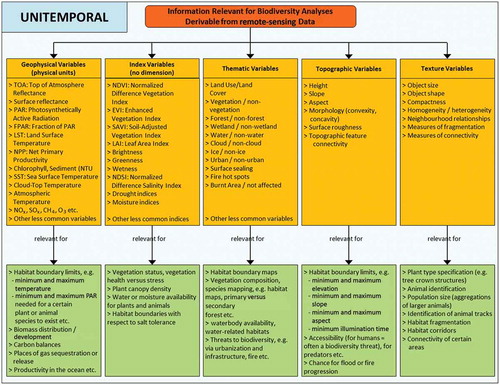
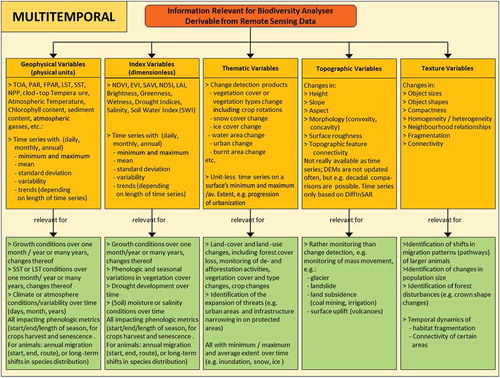
Figure 2. Information relevant for biodiversity analysis that can be gained from multitemporal remotely sensed data up to dense time series of data. Multitemporal data allow the monitoring of objects and habitats over time, and when long-term time series are available one can even observe trends (e.g. temperature shifts, snow cover duration shifts, etc.), and therefore slight geographic shifts of habitats.

Geophysical variables are defined by physical units quantifying LST, SST, atmospheric temperature (AT)), or available photosynthetically active radiation (PAR). Index variables are dimensionless and provide a pseudo-quantitative measure of the state of an ecosystem; e.g. the NDVI represents vegetation state and vigour. While geophysical variables and index variables are derived via clearly defined mathematical formulae, thematic variables are usually extracted with a higher degree of analyst bias. Thematic variables are for example land-cover and land-use information, derived either in the context of complex supervised multi-class classifications or as binary masks (water/non-water, urban/non-urban). In this category also falls the direct observation of biodiversity such as – especially in the case of vegetation – the supervised mapping of individual species based on knowledge of their spectral characteristics. Topographic variables such as height, slope, aspect, or surface roughness can be derived from DEMs (generated from either radar or optical stereo data), and texture variables such as object size, homogeneity, heterogeneity, or neighbourhood relationships depend on image segmentation or distinct object detection and subsequent object-oriented analysis. These latter variables are often used for direct vegetation biodiversity assessment (e.g. tree type differentiation based on crown size and shape). Fragmentation and connectivity are also extremely important measures, since ‘landscape fragmentation, through the disruption of habitat connectivity, can impact species dispersion and habitat colonization, gene flows and population diversity, and species mortality and reproduction’ (Nagendra et al. 2013, 50). Furthermore, it has been found that landscape and habitat heterogeneity is a driving factor for species richness (Leyequien et al. 2007). The green boxes in Figure 1 depict which biodiversity-relevant information can be retrieved based on these variables. Geophysical and topographic variables especially allow for the approximation of habitat boundary limits, for example defined by temperature, altitude, precipitation, or slope limits. The same applies for index variables, which furthermore depict the direct status of ecosystems. Thematic variables – including land-cover information – characterize an ecosystem and also elucidate resource availability (e.g. distance to waterbodies) or proximity to threats (humans, infrastructure). Texture variables can support the differentiation of species, estimation of population size or status, as well as the derivation of habitat fragmentation or connectivity.

Figure 2, which is similar to Figure 1 except that it is for multitemporal rather than unitemporal sources of data, depicts the five groups of variables as well as the relevant information for biodiversity analysis. It is the opportunity to observe the dynamics of variables that makes remote sensing a powerful tool for biodiversity-related studies. Whereas unitemporal studies only allow the assessment of the current situation, the multitemporal – and in the optimal case the time series – capability of some sensors allows a much larger range of biodiversity-relevant applications considering the past as well as the future (see Figure 2).

As depicted in the green boxes of Figure 2, multitemporal analysis of geophysical, index, thematic, topographic, and texture variables allows statements on variable conditions over the course of one month, one year, or even one or several decades, including the calculation of daily, weekly, monthly, and annual means, deviations, anomalies, general variability, and – given a long enough observation time span – even trends (e.g. LST annual range). Changes in growth conditions, phenologic metrics (e.g. start of season, mid of season, end of season), or growing season length can be observed over multiple years, and shifts in vegetation habitats can be depicted. One-land-cover-class monitoring, for example of water surfaces, including waterbodies and floods, allows the derivation of monthly, annual and even decadal minimum and maximum waterbody extent, flood frequency, and inundation variability. The same applies to land-cover and land-use change patterns that persist for decades and can be projected to continue into the future (e.g. urban sprawl or glacial retreat). Multitemporal elevation information allows the monitoring of surface displacement induced by land subsidence, which is often driven by groundwater, oil or gas extraction, other mining activities, or urban sprawl (heavy structures compacting the ground). While subsidence phenomena might not directly affect biodiversity, they are of relevance especially in the coastal zone. Many coastal ecosystems on shallow coastal shelves or in river deltas are under threat of ‘drowning’, as subsidence and sea level rise combine and lead to aggravated land submersion. Several sensors allow the monitoring of habitat development up to four decades into the past.

Next to highest resolution sensors, which partially enable mapping at the species level, especially sensors allowing long-term monitoring can be the main workhorses for extracting biodiversity-related environmental dynamics and delineating past, present, and future habitats. However, comprehensive overviews of all the different Earth observation satellite sensors and their data hardly exist. But it is exactly this amalgamated information on sensor types, specific sensors and their spatial and temporal resolution, time span of operation, and data availability that is essential for biologists, conservationists, environmental scientists, and even many remote-sensing experts who need to make decisions about which data can be employed to address their most pressing questions. Although some grey literature documents and websites with sensor overviews have been published by large space agencies such as the National Aeronautics and Space Administration (NASA), European Space Agency (ESA), Japan Aerospace Exploration Agency (JAXA) etc., they mostly present the sensors they themselves operate. To our knowledge, no overarching, well-structured overview of all available spaceborne remote-sensing sensors tailored to the needs of the biodiversity community exists. We provide this in the following sections and concentrate on up-to-date sensors (sensors, which are still in orbit, or long sensors lines, which have been frequently exploited).

4. Satellite sensor categorization: optical/infrared, thermal infrared, and radar sensors

A review and comparison of past, present, and future sensors used for Earth observation is essential for providing a good overview of their technical capabilities to the remote-sensing and user communities, exposing existing gaps, and listing requirements for future missions. Several authors have provided sectorial reviews of different types of sensors. About a decade ago, Melesse et al. (2007) reviewed the history of remote sensing and the development of different sensors for environmental and natural resource mapping and data acquisition. Gillespie et al. (2007) presented an overview of recent satellites with passive sensors that provide panchromatic, visible, near-infrared, shortwave infrared, and thermal infrared (TIR) information suitable for the remote sensing of hazards. Goetz (2009) discussed the development of airborne and spaceborne hyperspectral sensors and data analysis techniques during the last 30 years and pointed out current limitations and future needs. CubeSats have been addressed by Sandau (2010) and Cracknell (2010), amongst others. A comprehensive work of Kramer (2002) presents an overview of available satellite sensors, but this does not contain developments of the past decade. However, an updated edition of the book will be published around the end of 2014. Only a few articles illustrate the use and potential of airborne and spaceborne sensors for observations in the field of biodiversity and conservation. Ten years ago, Turner et al. (2003) presented a review of sensors available for indirect biodiversity monitoring via the derivation of biophysical parameters, and Wang et al. (2010) reviewed spaceborne remote sensing for ecology, biodiversity, and conservation studies, mainly focusing on high-resolution, hyperspectral, lidar, and small CubeSat sensors. However, no publication exists that is half-way up to date and presents a holistic overview of all spaceborne available optical, infrared, thermal, and radar imaging sensors as well as highlighting their most suitable fields of application related to biodiversity-type assessments.

Based on information from published Science Citation Index studies and sectorial reviews, grey literature, and websites provided by space agencies and sensor operators, we compiled timeline charts of currently active sensors acquiring data in the optical and near-infrared domain (Figure 3), the TIR domain (Figure 4), and radar domain (Figure 5). After a first overview, we go into detail on spatial and temporal sensor characteristics and preferred application domains (Section 5). This is followed by a section on data availability, access, and costs (Section 6).

Figure 3. Timelines of major Earth observation satellites with optical/multispectral sensors.

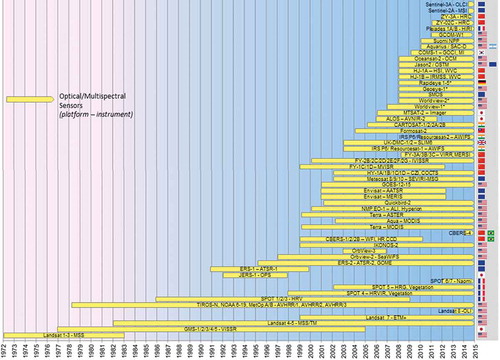
Figure 4. Timelines of major Earth observation satellites with thermal sensors.

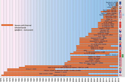
Figure 5. Timelines of major Earth observation satellites with radar and passive microwave sensing instruments.

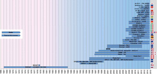
Figure 3 presents an overview of optical and (near-/mid-) infrared spaceborne sensors, their active data acquisition period, as well as their country of origin. As a general rule, we only list sensors that are still active (indicated by an arrow at the right end of the yellow bar). However, in exceptional cases, past sensors were included in the case of missions designed to provide long-term data continuity and which are more or less seamlessly complemented by later missions.

It can be seen that only a few optical and multispectral sensors really allow long-term monitoring. Only the multispectral NOAA-AVHRR (National Oceanic and Atmospheric Administration Advanced Very High Resolution Radiometer) sensor offering 1 km spatial resolution at a better than daily revisiting time enables an area to be monitored back in time to the late 1970s. Due to its very high temporal resolution (at least daily revisits, and twice a day for many places), even in the most cloud-covered regions of Earth, it is likely to acquire cloud-free imagery at least once a month. At the same time, 1 km spatial resolution is too coarse for many species or habitat mapping applications. Only the Landsat fleet, starting with the Landsat MSS, followed by TM and ETM+, and now continued via the Landsat-DCM (8) satellite launched in February 2013, allows long-term monitoring of an area for over 30 years at a spatial resolution averaging 30 m up to 10 m (ETM+ and LDCM panchromatic). The development of the Landsat mission has been reviewed by Wulder et al. (2011), Irons, Dwyer, and Barsi (2012), and Loveland and Dwyer (2012). The latter discussed the strategy of the Landsat programme with its numerous missions as well as the progress of the Landsat archive of the US Geological Survey (USGS) and specified US Federal efforts including the development of Landsat 9 and 10 in the future. It is for this reason that in all remote-sensing journal articles, it is the Landsat sensor that has been used most frequently for local to regional analyses. The exploitation of medium-resolution AVHRR time series has also been undertaken by numerous authors, however, not as frequently as published studies based on medium-resolution MODIS data. MODIS – contrary to AVHRR – can only cover the past decade, but it offers spatial resolution up to 250 m. Numerous value-added products are freely made available by the MODIS science team, and the sensor has been continuously orbiting since 2000 so that data intercalibration challenges, as occur with the fleet of consecutive AVHRR sensors, are not an issue.

Nagendra et al. (2013) underline that there is a broad assumption in the community of conservationists that higher spatial resolution is always better, and thus there is a current preference for ordering the highest available spatial resolution data, such as QuickBird, IKONOS, GeoEye, or WorldView. However, many of these sensors lack an infrared or thermal band, which can be very useful for vegetation type discrimination. Furthermore, the value of high-temporal resolution data (time series) is still underestimated to date.

There is a clear nation-related tendency: although one third of the sensors or sensor-lines presented are operated by the USA, European and here especially French sensors have also played a role since the beginning of remote-sensing imaging. Since the year 2000, already 14 of the listed optical/multispectral spaceborne sensors have been launched and operated by China. India also launched at least seven optical/multispectral sensors into orbit within only the past 10 years.

The high value of thermal sensors and extractable information such as monotemporal LST, SST, emissivity, thermal inertia, and thermal anomalies, as well as temperature time series, is often underestimated (Kuenzer and Dech 2013; Kuenzer et al. 2008). However, as upper and lower LST/SST values are defining factors for many vegetation and animal habitats, temperature information should be part of any biodiversity-related analyses. Figure 4 depicts all current TIR Earth observation sensors in orbit. Furthermore, thermal data are a valuable tool for fire ecology applications (forest fires, slash and burn, etc.). The same patterns as with optical/shortwave and mid-infrared sensors can also be observed in the domain of thermal sensors. Except for AVHRR and Landsat, no other sensor or sensor line offers the chance of long-term monitoring of thermal patterns covering three to four decades. While AVHRR offers on average two thermal observations per day, Landsat still has a 16 day repeat cycle, and especially in cloudy latitudes, completely cloud-free observations might therefore only be available a few times per year.

Just as for optical and near-/mid-infrared data, the MODIS sensor is also used for many LST, SST, and hot spot detection studies. Up to four observations per day (two from the Terra platform, two from the Aqua platform) as well as two suitable bands (31, 32) in the TIR domain allow the derivation of complex thermal products.

Also for thermal sensors (most of them flown jointly with optical/multispectral sensors), a clear dominance of USA-operated instruments catches the eye. Europe follows second, but China’s launch activities in the past decade in the TIR domain are also outstanding. While AVHRR, MODIS, and Landsat, as well as the Aster satellite (which has five thermal bands and is thus often employed for emissivity spectra applications), are mainly used for global, regional and, local thermal analysis, respectively, thermal data from the geostationary sensor Meteosat enable the acquisition of thermal imagery of a fixed view (e.g. the European and African part of the northern and southern hemispheres). Meteosat data are usually analysed by the meteorological science community.

Figure 5 depicts all passive and active microwave sensors that either are still in orbit or are of broader significance as they were employed for numerous studies. Radar data – especially if combined with optical data – offer several advantages, such as the extraction of the three-dimensional structure of habitats (Nagendra et al. 2013). The workhorse for the radar remote-sensing community has been the European Remote Sensing Satellite (ERS) sensor, with data available since the early 1990s. ERS data provided by ESA have been used for numerous global product developments and applications. ESA has granted easy and low-cost access to ERS-1 and ERS-2 data (data access will be addressed in subsection 6), and the same applies to ESA’s Envisat ASAR (Advanced Synthetic Aperture Radar) data, available for the time period 2002 to 2012. Thus, it is especially these two sensors that are extensively used for environmental analysis. Since 2007, TerraSAR-X sensor data have also been increasingly used for local studies. Other radar sensor data, such as from Canada’s Radarsat, Italy’s Cosmo SkyMed, as well as many other sources listed in Figure 6, are either very costly to acquire or not easily accessible. Contrary to optical/infrared data (Figure 4), which provide an archive going back 40 years into the past, radar-based time-series analyses can only provide an archive going back to the early 1990s (ERS). This relatively short time span, as well as additional years with data gaps, rules out these radar time series as a data source for the observation of climate change-relevant trends. The low spatial resolution of ERS data – 25 km – further decreases the attractiveness of derived products for stakeholders and decision-makers. However, for long-term habitat analysis, typical data products such as soil moisture, biomass, sea ice, or waterbody maps are of great importance for monitoring habitat boundary shifts over time.

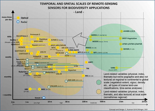
Figure 6. Optical/infrared (yellow) and radar (blue) sensors used for land-related applications.

5. Satellite sensor categorization: application domains, spatial and temporal resolution, and suitability for various biodiversity applications

We designed Figures 6 to 10 to present a comprehensive overview of satellite sensors used in different spheres (land, water, and air), differentiating sensor types (optical/multispectral, radar (active and passive), thermal), giving each sensor’s spatial and temporal resolution, and illustrating the major application domains the data are used for. The figures should be read and understood in the following way.

• The X-axis represents spatial resolution (from better than 1 m to over 50 km).

• The Y-axis represents temporal resolution (revisit time) (from better than daily to less than monthly).

• Dots represent sensors (with the sensor name next to the dot); lines present the spatial range, if a sensor offers data at more than one spatial resolution. The dot is located at the highest resolution the sensor has to offer.

• Yellow dots represent optical/multispectral sensors, red dots represent thermal sensors, blue dots represent radar sensors (passive radar sensors in italics).

• Coloured ellipses represent preferred applications (see legend).

• Arrows within the individual figures represent gaps (requiring the development of sensors with higher spatial or temporal resolution).

• Tables at the end of this article list all relevant sensors in detail.

Figure 6 and Table 1 show that a large fleet of optical and radar sensors is available for land applications (thermal sensors are identified separately in Figure 8). While one group of optical/multispectral sensors is characterized by low-to-medium spatial resolutions (1 km to 100 m) but near global coverage at weekly to daily temporal resolutions (green ellipse), other radar and optical sensors have spatial resolutions between 30 m and better than 1 m. However, this group of sensors (yellow ellipse) does not allow daily global coverage, not even monthly or annual global coverage. While sensors such as AVHRR and MODIS acquire almost all data frames and thus deliver global coverage, sensors such as Landsat, Aster, TerraSAR-X, Radarsat, and WorldView only acquire data when tasked. Thus, it is rare to achieve daily, weekly, monthly, or even annual coverage with data from these sensors. The Landsat science team has published global coverage mosaics composed of data sets acquired during time spans covering up to five years. Other global products based on this higher spatial resolution data – for example, the global urban footprint (Esch et al. 2010) – are also a conglomerate mosaic of scenes from multiple years.

Table 1. “Land” application-related sensors.

Sensor/instrument	Sensor type	Spatial resolution	Minimum local revisit time (days)	Maximum swath width (km)	Platform	Agency	Launch date
QuickBird	Optical	0.6–2.4 m	2.5–5.6	18	QuickBird	Digital Globe	2001
IKONOS	Optical	1–4 m	3	11	IKONOS	GeoEye	1999
GeoEye-1	Optical	0.41–1.65 m	2.1–8.3	15.2	GeoEye-1	GeoEye	2008
WorldView 2	Optical	0.5–1.8 m	1.1–3.7	16.4	WorldView-2	Digital Globe	2009
HiRI	Optical	0.7–2.8 m	2	20–100	Pleiades 1A/1B	CNES	2011/2012
HRC (ZY-3A)	Optical	2.1 (nadir)–3.5 m (forward/backward)	59 (4–5 in special cases)	52	ZY-3A	CRESDA	2012
HRC (ZY1-02 C)	Optical	2.36 m	26	54	ZY1-02C	CRESDA	2011
Naomi	Optical	2–8 m	3 (daily revisit capability SPOT 6/7)	120	SPOT 6/7	EADS Astrium	2012/2014
SPOT-HRG	Optical	2.5 m/5 m/10 m/20 m	2–3	60	SPOT 5	EADS Astrium	2002
Cartosat-1	Optical	2.5 m	5	30	CARTOSAT 1	ISRO	2005
Cartosat-2	Optical	1 m	4	9.6	CARTOSAT 2/2A/2B	ISRO	2007/2008/2010
RapidEye	Optical	5 m	1–5.5	77	RapidEye 1/2/3/4/5	RapidEye	2008
Formosat	Optical	2–8 m	1	24	Formosat-2	NSPO	2004
LISS-IV	Optical	5.8 m	5	23–70	Resourcesat-1/2	ISRO	2003/2011
PAN/MS (ZY1-02 C)	Optical	5–10 m	26	60	ZY1-02C	CRESDA	2011
MSC (ZY-3A)	Optical	6 m	59 (4–5 in special cases)	51	ZY-3A	CRESDA	2012
PANMUX	Optical	5–10 m	5	60	CBERS-4	CRESDA/INPE	2014
MSI	Optical	10 m/20 m/60 m	10 (5 with two satellites)	290	Sentinel-2A	ESA	2014
HR CCD	Optical	20 m	3–26	113	CBERS-1/2/2B	CRESDA/INPE	1999/2003/2007
SPOT-HRVIR	Optical	10 m/20 m	2–3	60	SPOT 4	EADS Astrium	1998
SPOT-HRV	Optical	10 m/20 m	2–3	60	SPOT 1–3	EADS Astrium	1986/1990/1993
MUXCAM	Optical	20 m	5	120	CBERS-4	CRESDA/INPE	2014
ASTER	Optical	15 m/30 m/90 m	16	60	Terra	NASA	1999
LISS-III	Optical	23,5 m	24	141	Resourcesat-1/2	ISRO	2003/2011
AVNIR-2	Optical	10 m	2	70	ALOS	NASDA	2006
ALI	Optical	10 m/30 m	16	37	NMP EO-1	NASA	2000
OLI	Optical	15 m/30 m	16	185	Landsat 8	USGS/NASA	2013
TM	Optical	30 m/120 m	16	185	Landsat 5	USGS/NASA	1984
ETM+	Optical	30 m/60 m	16	185	Landsat 7	USGS/NASA	1999
WVC	Optical	30 m	4	700	HJ-1A, HJ-1B	CAST	2008
SLIM6	Optical	32 m	5	320/600	UK-DMC-1/UK-DMC-2	BNSC	2003/2009
AWiFS	Optical	56 m	5	740	Resourcesat-1/2	ISRO	2003/2011
WFI2	Optical	64 m	5	866	CBERS-4	CRESDA/INPE	2014
IRMSS (HJ-1 B)	Optical	150–300 m	4	720	HJ-1B	VAST	2008
MERSI	Optical	250 m–1.1 km	1	2800	FY-3A/3B/3C	CMA/CNSA	2008/2010/2013
WFI	Optical	258 m	5	890	CBERS-1/2/2B	CRESDA/INPE	1999/2003/2007
MODIS	Optical	250–1000 m	1–2	2330	Terra	NASA	1999
VIIRS	Optical	375–750 m	2	3000	Suomi NPP	NASA/NOAA	2011
AATSR	Optical	1 km	3	512	Envisat	ESA	2002
ATSR-1	Optical	1 km	3	500	ERS-1	ESA	1991
ATSR-2	Optical	1 km	3	512	ERS-2	ESA	1995
AVHRR/1	Optical	1.1 km	<1	2600	TIROS-N, NOAA-6/8/10	NOAA	1978–1986
AVHRR/2	Optical	1.1 km	<1	3000	NOAA-7/9/11/12/14	NOAA	1981–1994
AVHRR/3	Optical	1.1 km	<1	3000	NOAA-15/16/17/18/19, MetOp A/B	NOAA, EUMETSAT	1998–2012
MVISR	Optical	1.1 km	3–4	3200	FY-1D	CMA/NRSCC	2002
SPOT-Vegetation	Optical	1 km	1	2250	SPOT 4, SPOT 5	EADS Astrium	1998/2002
Imager	Optical	1–4 km	Geostationary, every 30 min	Full Earth disk	MTSAT-2	JMA	2006
RadarSat-1	Radar	8–100 m	24	45–500	Radarsat 1	CSA	1995
RadarSat-2	Radar	3–100 m	24	50–500	Radarsat 2	CSA	2007
TerraSAR-X	Radar	1–18 m	11	10–100	TerraSAR-X	DLR	2007
Tandem-X	Radar	1–18 m	11	10–100	Tandem-X	DLR	2010
ASAR	Radar	30–1000 m	2–7	5–405	Envisat	ESA	2002
SAR 2000	Radar	1–100 m	5 (0.5 in full constellation with SkyMed 1–4)	10–200	Cosmo-SkyMed 1/2/3/4	ASI	2007/2007/2008/2010
ALOS-PALSAR	Radar	10–100 m	46	70–350	ALOS	NASDA	2006
AMI-SAR	Radar	30–1000 m	35	100	ERS-1/2	ESA	1991/1995
RISAT-1	Radar	3–50 m	25	30–240	RISAT-1	ISRO	2012
RISAT-2	Radar	3–8 m	25	10–650	RISAT-2	ISRO	2009
SEASAT	Radar	25 m	105	100	SEASAT-1	NASA	1978
RORSAT	Radar	n.a.	n.a.	n.a.	KOSMOS 102–1932	n.a.	1967–1988
HSI	Optical	100 m	4–31	50–500	HJ-1A	CRESDA	2008
Hyperion	Optical	30 m	16	7.5	NMP EO-1	NASA	2000

HRG, High Resolution Geometrical; IMC, Infrared Multispectral Camera; LISS, Linear Imaging Self Scanner; MERSI, Medium-Resolution Spectral Imager; HRVIR, High-Resolution Visible; WFI2, Wide-Field Imager Camera 2; HRV, High Resolution Visible; MVISR, Multispectral Visible and Infrared Scan Radiometer; ASTER, Advanced Spaceborne Thermal Emission and Reflection Radiometer; ASAR, Advanced Synthetic Aperture Radar; ALI, Advanced Land Imager; LISS-IV, Linear Imaging Self Scanner III; OLI, Operational Land Imager; AVHRR, Advanced Very High-Resolution Radiometer; TM, Thematic Mapper; HRC, High-Resolution Camera; ETM, Enhanced Thematic Mapper; HR Pan, High-Resolution Panchromatic; AWFI, Advanced Wide-Field Imaging Camera; PAN/MS, Panchromatic/Multispectral; AWiFS, Advanced Wide-Field Imager; MUX, Multispectral; MODIS, Moderate-Resolution Imaging Spectroradiometer; PANMUX, Panchromatic and Multispectral; AATSR, Advanced Along-Track Scanning Radiometer; HR CCD, High Resolution CCD; ATSR-1, Along-Track Scanning Radiometer-1; MUXCAM, Multispectral Camera; ATSR-2, Along-Track Scanning Radiometer-2; MVISR, Multispectral Visible and Infrared Scan Radiometer; VHRR, Very High-Resolution Radiometer; VIIRS, Visible/Infrared Imager Radiometer Suite; WFI, Wide-Field Imager Camera; HSI, Hyperspectral Imager; WVC, Wide-View CCD Camera; HiRI, High-Resolution Imager; SLIM6, Surrey Linear Imager Multispectral 6 channels.

For land-related biodiversity applications, it is the ‘green ellipse sensors’ which are suitable for mapping national to global scale habitat boundary conditions via physical, index, and thematic variables. As the sensors allow daily coverage, which is provided for the past 10 to 40 years, it is possible to undertake time-series analysis and derive means, deviations, anomalies, variability, and possibly even climate-change-related trends (Cracknell 1997). For example, Dietz (2013) used 30 years of daily available AVHRR-derived snow cover information to show that the snow season in Central Asia has shifted during the last decades: in Central Asia over the past 30 years, it can be observed that the first snowfall comes about two weeks later, and that there is also a shift in the start of snowmelt, which takes place about two weeks earlier. Such climate change-related shifts can only be extracted from data that are available daily.

Sensors in the yellow ellipse allow detailed mapping and multitemporal monitoring at the local scale. These sensors definitely allow mapping down to the species level if the species covers a large enough area (a few pixels), and also allow the derivation of texture-related variables of image segments (objects), which is also important information for species discrimination. While the highest resolution optical sensors such as GeoEye, WorldView, QuickBird, or IKONOS theoretically also allow the detection of individual animals and the counting of populations, this is still a niche application, and obtaining good data for mammal herds or flocks of migratory birds is rather a product of chance than something that can be planned.

The black arrow indicates that there is still an opportunity to improve the spatial resolution of daily available global coverage sensor data.

Figure 7 and Table 2 identify sensors predominantly used for the remote sensing of oceans, lakes, and other waterbodies. Whereas passive radiometers (in italics) as well as lowest resolution active radars are mainly used to derive wind speed and direction, wave height and direction, sea ice, and coastal moisture (right, blue ellipse), medium-resolution optical sensors mainly contribute to water colour mapping, the derivation of chlorophyll and sediment load, or the identification of large algae carpets (yellow ellipse). The highest resolution SAR sensors listed in the lower left turquoise ellipse are suitable for local derivation of waterbody extent, inundation and flood dynamics, as well as the detection of objects on water surfaces that might threaten marine or limnic ecosystems (ships, oil spills, floating garbage), whereas the highest resolution optical sensors are used for shallow water bathymetry derivation and local water colour analysis.

Figure 7. Optical/infrared (yellow) and radar (blue) sensors for ocean/waterbody applications.

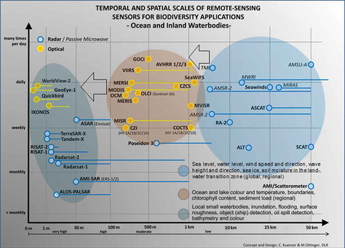
Table 2. “Ocean and inland waterbodies” application-related sensors.

Sensor/instrument	Sensor type	Spatial resolution	Minimum local revisit time (days)	Maximum swath width (km)	Platform	Agency	Launch date
Ocean and Inland Waterbodies
MODIS	Optical	250–1000 m	1–2	2330	Terra, Aqua	NASA	1999/2002
CZI	Optical	250 m	7	500	HY-1A/1 B/1 C/1D	CAST	2002/2007/2014/2014
MERIS	Optical	300 m	3	575–1150	Envisat	ESA	2001
OLCI	Optical	300 m	2.2 (1.9 with two satellites)	1270	Sentinel-3A	ESA	2014
OCM	Optical	236 m	2	1420	Oceansat-2	ISRO	2009
GOCI	Optical	500 m	Geostationary, 3 per day	1440	COMS-1	Astrium/KARI/KORDI	2010
OLS	Optical	560 m	Geostationary,<1	2960	DMSP-F01-19	NOAA	1976–2014
MISR	Optical	275 m/1.1 km	2–9	360	Terra	NASA	1999
MERSI	Optical	250–1.1 km	1	2800	FY-3A/3 B/3 C	CMA/CNSA	2008/2010/2013
CZCS	Optical	825 m	1	1600	Nimbis-7	NASA	1978
SeaWIFS	Optical	1.1 km	1	2800	OrbView-2	NASA	1997
MVISR	Optical	1.1 km	3–4	3200	FY-1 C/1D	CMA/NRSCC	1999/2002
SLIM-6	Optical	32 m	5	320/600	UK-DMC-1/UK-DMC-2	BNSC	2003/2009
Radarsat-1	Radar	8–100 m	24	45–500	Radarsat-1	CSA	1995
Radarsat-2	Radar	3–100 m	24	50–500	Radarsat-2	CSA	2007
ASAR	Radar	30–1000 m	2–7d	5–405	Envisat	ESA	2002
RA-2	Radar	10 km	2–7d	10	Envisat	ESA	2002
Poseidon-3	Radar	600 m-6 km	10	300	Jason 2	NASA/NOAA/CNES/EUMETSAT	2008
ALT	Radar	16 km	14	16	HY-2A	NSOAS, CAST	2011
TerraSAR-X/ Tandem-X	Radar	1–16 m	11	10–100	TerraSAR-X/Tandem-X	DLR	2007/2011
MIRAS	Passive microwave	33–50 km	1–2	1000	SMOS	ESA	2009
SCAT	Radar	50 km	14	1300	HY-2A	NSOAS, CAST	2011
AMI/Scatterometer	Radar	50 km	35	1000	ERS-1/ERS-2	ESA	1991/1995
AMI/SAR	Radar	30–1000 m	35	100	ERS-1/ERS-2	ESA	1991/1995
ASCAT	Radar	25/50 km	4	500	Metop-A/B	EUMETSAT	2006/2012
Seawinds	Radar	25 km	1–2	1600	QuikSCAT, ADEOS-II	NASA	1999/2002
AMSU-A	Passive microwave	50 km	1	2100	NOAA 15/16/17/18, MetopA/B	NOAA, EUMETSAT	1998–2012
MWRI	Passive microwave	15–85 km	1	1400	FY-3A/3 B/3 C	CMA/CNSA	2008/2010/2013
VIIRS	Optical	375 m–1.6 km	1	3000	Suomi NPP	NASA/NOAA	2011
AVHRR/1	Optical	1.1 km	<1	2600	TIROS-N, NOAA-6/8/10	NOAA	1978–1986
AVHRR/2	Optical	1.1 km	<1	3000	NOAA-7,9,11,12,14	NOAA	1981–1994
AVHRR/3	Optical	1.1 km	<1	3000	NOAA-15/16/17/18/19, MetOp A/B	NOAA, EUMETSAT	1998–2012
COCTS	Optical	1.1 km	7	1400	HY-1A/1 B/1 C/1D	CAST	2002/2007/2014/2014
TMI	Passive microwave	5 km	0.5–1	790	TRMM	JAXA/NASA	1997
AMSR-2	Passive microwave	5–50 km	1–2	1450	GCOM-W1	JAXA	2008
RISAT-1	Radar	3–50 m	25	30–240	RISAT-1	ISRO	2012
RISAT-2	Radar	3–8 m	25	30–-650	RISAT-2	ISRO	2009
PALSAR-2	Radar	1–100 m	14	25–350	ALOS-2	JAXA	2012
PALSAR	Radar	10–100 m	46	70–350	ALOS	JAXA	2006

AVHRR, Advanced Very High-Resolution Radiometer; MVISR, Multispectral Visible and Infrared Scan Radiometer; MODIS, Moderate-Resolution Imaging Spectroradiometer; ASAR, Advanced Synthetic Aperture Radar; MERIS, Medium-Resolution Imaging Spectrometer; RA-2, Radar Altimeter-2; OCM, Ocean Colour Monitor; ALT, Radar Altimeter; GOCI, Geostationary Ocean Colour Imager; MIRAS, Microwave Imaging Radiometer with Aperture Synthesis; MISR, Multi-Angle Imaging SpectroRadiometer; Ascat, Advanced Scatterometer; MERSI, Medium Resolution Spectral Imager; AMI, Active Microwave Instrumentation; SeaWiFS, Sea-Viewing Wide Field-of-View Sensor; TMI, TRMM Microwave Imager; Scat, Scatterometer; AMSR-2, Advanced Microwave Scanning Radiometer-2; AMSU-A, Advanced Microwave Sounding Unit-A; RISAT, Radar Imaging Satellite; MWRI, Microwave Radiometer Imager; PALSAR, Phased Array type L-band Synthetic Aperture Radar; VIIRS, Visible/Infrared Imager Radiometer Suite; CZI, Coastal Zone Imager; COCTS, China Ocean Colour and Temperature Scanner; CZCS, Coastal Zone Colour Scanner.

Thermal sensors for the derivation of LST, SST, and thermal anomalies are identified in Figure 8 and listed in Table 3. As these are usually mounted on the same platforms as their multispectral counterparts (e.g. AVHRR, MODIS, Landsat, etc.), they also have similar revisit times. A large number of sensors exist that acquire data daily with near global coverage (yellow ellipse). These data at spatial resolutions between 50 km and 1 km enable the derivation of large-area LST and SST patterns (cloud cover permitting), as well as the extraction of large thermal anomalies, such as caused by extensive forest fires. Thermal sensors on Landsat, Aster, CBERS, or Sentinel-2 are more suitable for local studies of temperature patterns or local hot spot extraction. They are also suitable for the detection of thermal water pollution in rivers and lakes.

Figure 8. Thermal sensors and the opportunities they offer for biodiversity-related applications.

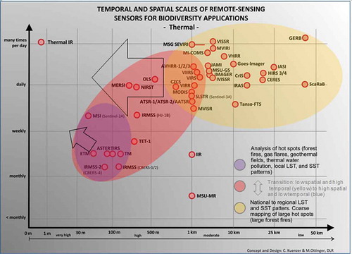
Table 3. “Thermal” application-related sensors.

Sensor/instrument	Sensor type	Spatial resolution	Minimum local revisit time (days)	Maximum swath width (km)	Platform	Agency	Launch date
Surface Temperature
ETM+	Optical	60 m	16	185	Landsat 7	USGS/NASA	1999
MSI	Optical	60 m	10 (5 with two satellites)	290	Sentinel-2A	ESA	2014
TM	Optical	120 m	16	185	Landsat 5	USGS/NASA	1984
ASTER	Optical	90 m	16	60	Terra	NASA	1999
IRMSS-2	Optical	80 m	26	120	CBERS-4	CRESDA/INPE	2014
TIRS	Optical	100 m	16	185	Landsat 8	USGS/NASA	2013
IRMSS	Optical	160 m	26	120	CBERS-1/2	CRESDA/INPE	1999/2003
CIRC	Optical	200 m	14	128	ALOS-2	JAXA	2014
MERSI	Optical	250 m	1	2800	FY-3A/3 B/3 C	CMA/CNSA	2008/2010/2013
IRMSS (HJ-1B)	Optical	300 m	4	720	HJ-1B	CRESDA/CAST/NRSCC	2008
TET-1	Optical	356 m	10	180	TET-1	DLR	2012
NIRST	Optical	351 m	<1–2	182–1000	Aquarius	NASA/CONAE	2011
OLS	Optical	560 m	Geostationary, <1	2960	DMSP F01-19	NOAA	1976–2014
CZCS	Optical	825 m	1	1600	Nimbis-7	NASA	1978
ATSR-1	Optical	1 km	3	500	ERS-1	ESA	1991
ATSR-2	Optical	1 km	3	512	ERS-2	ESA	1995
AATSR	Optical	1 km	3	500	Envisat	ESA	2002
SLSTR	Optical	1 km	1.8 (0.9 with two satellites)	1420	Sentinel-3A	ESA	2014
IIR	Optical	1 km	16	64	CALIPSO	CNES	2006
MODIS	Optical	1 km	1–2	2330	Terra, Aqua	NASA	1999/2002
AVHRR/1	Optical	1.1 km	<1	2600	TIROS-N, NOAA-6/8/10	NOAA	1978–1986
AVHRR/2	Optical	1.1 km	<1	3000	NOAA-7/9/11/12/14	NOAA	1981–1994
AVHRR/3	Optical	1.1 km	<1	3000	NOAA15/16/17/18/19, Metop A/B	NOAA/EUMETSAT	1998–2012
MSG-SEVIRI	Optical	1–3 km	Geostationary, <1	Full Earth disk	Meteosat-8/9/19	ESA/EUMETSAT	2002/2005/2012
VIRR	Optical	1.1 km	1	2800	FY-3A/3B/3C	CMA/CNSA	2008/2010/2013
MVISR	Optical	1.1 km	3–4	3200	FY-1C/1D	CMA/NRSCC	1999/2002
VIIRS	Optical	1.6 km	<1	3000	Suomi NPP	NASA/NOAA	2011
VIRS	Optical	2 km	<1	720	TRMM	NASA	1997
IVISSR	Optical	5 km	Geostationary, <1	Full Earth disk	FY-2B/2C/2D/2E/2F/2G	NRSCC/CAST/NSMC-CMA	2000/2004/2006/2008/2012/2014
MVIRI	Optical	5 km	Geostationary, every 30 min	Full Earth disk	Meteosat-1/2/3/4/5/6/7	EUMETSAT, ESA	1977/81/88/89/91/93/97/98/ 2006/2007
MSU-MR	Optical	1 km	37	3000	Meteor 3M, Meteor-M N1	ROSHHYROMET a.o.	2001/2009
MSU-GS	Optical	4 km	Geostationary <1	Full Earth disk	Elektro-L N1	ROSHHYROMET a.o.	2011
MI-COMS	Optical	4 km	Geostationary, every 30 min	Full Earth disk	COMS	KARI/ITT	2010
JAMI	Optical	4 km	Geostationary, <1	Full Earth disk	MTSAT-1R	JMA	2005
IMAGER	Optical	4 km	Geostationary, <1	Full Earth disk	MTSAT-2	JMA	2006
VISSR	Optical	5 km	Geostationary, every 30 min	Full Earth disk	GMS-1/2/3/4/5	JMA	1977/1981/1984/1989/1995
VHRR	Optical	8 km	Geostationary, every 30 min	Full Earth disk	Insat-1A/1B/1C/1D/2A/2B/2C/2D, Kalpana-1, Insat-3A	ISRO	1982/83/86/90/92/93/97/99, 2002/2003
GOES Imager	Optical	1–4 km	Geostationary, every 30 min	Full Earth disk	GOES 12/13/14/15	NOAA	2001/2006/2099/2010
Tanso-FTS	Optical	10.5 km	3	160	GOSAT	JAXA	2009
IRAS	Optical	14 km	1	952	FY-3A/3B/3C	NRSCC/CAST/NSMC-CMA	2008/2010/2013
CrIS	Optical	14 km	<1	2200	Suomi NPP	NASA/NOAA	2011
CERES	Optical	20 km	<1	3000	Suomi NPP	NASA/NOAA	2011
IASI	Optical	25 km	0.5/twice daily	2052	MetOP-A/B	EUMETSAT	2006/2012
HIRS/3	Optical	20.3 km	<1	2240	NOAA-15/16/17	NOAA	1998/2000/2002
HIRS/4	Optical	20.3 km	<1	2240	NOAA 18, MetOp A, NOAA 19, MetOp B	NOAA/EUMETSAT	2005/2006/2009/2012
GERB	Optical	40 km	Geostationary, every 5 min	Full Earth disk	Meteosat-8/9/10	EUMETSAT/ESA/RAL	2002/2005/2012
ScaRaB	Optical	40 km	1	2200	Megha Tropiques	CNES	2011

ETM+, Enhanced Thematic Mapper; VIIRS, Visible/Infrared Imager Radiometer Suite; TM, Thematic Mapper; AATSR, Advanced Along-Track Scanning Radiometer; ASTER, Advanced Spaceborne Thermal Emission and Reflection Radiometer; AVHRR, Advanced Very High-Resolution Radiometer; IRSCAM, Infrared Medium Resolution Camera; MSG-SEVIRI, Spinning Enhanced Visible and InfraRed Imager; TIRS, Thermal infrared sensor; VIRR, Visible and InfraRed Radiometer; IRMSS, InfraRed Multispectral Sensor; MVISR, Multispectral Visible and Infrared Scan Radiometer; MODIS, Moderate Resolution Imaging Spectroradiometer; IVISSR, Improved Multispectral Visible and Infrared Scan Radiometer; MERSI, Medium Resolution Spectral Imager; VHRR, Very High-Resolution Rdaiometer; NIRST, New Infrared Sensor Technology; IASI, Infrared Atmospheric Sounding Interferometer; VIRS, Visible and Infrared Scanner; MI, Meteorological Imager; OLS, Operational Linescan System; JAMI, Japanese Advanced Meteorological Imager; GERB, Geostationary Earth Radiation Budget; SLSTR, Sea and Land Surface Temperature Radiometer; VISSR, Visible-Infrared Spin Scan Radiometer.

As the black arrows in Figure 8 indicate, there is still space for the development of thermal sensors with a daily revisit time and higher spatial resolution.

Figure 9 and Table 4 identify sensors mostly used to derive atmospheric parameters. Data on cloud cover, water vapour, ozone, nitrous and sulphur oxides, as well as wind speed are rarely exploited outside the meteorological community. However, due to daily global coverage, such data might be interesting when combined with global tracking data on migratory birds covering large distances. Combining track data with wind speed data, or combining mammal or bird track with data reflecting air pollution, might give us new insight into the capability of animals as bio-sensors.

Figure 9. Atmosphere-related sensors and products of interest for biodiversity applications.

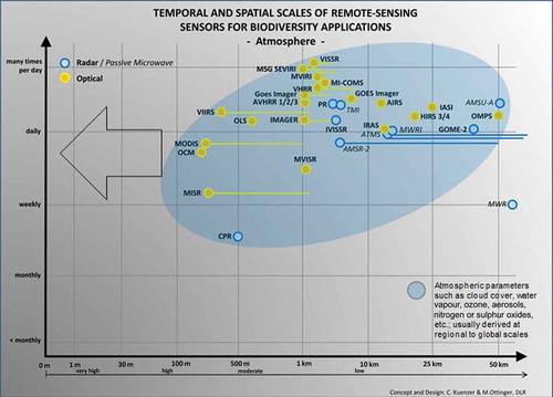
Table 4. “Atmosphere” application-related sensors.

Sensor/instrument	Sensor type	Spatial resolution	Minimum local revisit time (days)	Maximum swath width (km)	Platform	Agency	Launch date
Atmosphere
AVHRR/1	Optical	1.1 km	<1	2600	TIROS-N, NOAA-6/8/10	NOAA	1978–1986
AVHRR/2	Optical	1.1 km	<1	3000	NOAA-7/9/11/12/14	NOAA	1981–1994
AVHRR/3	Optical	1.1 km	<1	3000	NOAA-15/16/17/18/19, MetOp A/B	NOAA/EUMETSAT	1998–2012
MVISR	Optical	1.1 km	3–4	3200	FY-1D	CMA/NRSCC	2002
GOES Sounder	Optical	8 km	Full Earth disk in 8 h	Full Earth disk	GOES-12/13/14/15	NOAA	2001/2006/2009/2010
OCM	Optical	236 m	2	1440	Oceansat-2	ISRO	2009
VIIRS	Optical	375 m–1.6 km	<1	3000	Suomi NPP	NASA/NOAA	2011
OMPS	Optical	50 km	<1	250–2800	Suomi NPP	NASA/NOAA	2011
MVIRI	Optical	2.5 km/5 km	Full Earth disk every 30 min	Full Earth disk	Meteosat-7	ESA/EUMETSAT	1997
HIRS/3	Optical	20.3 km	<1	2240	NOAA-15/16/17	NOAA	1998/2000/2002
HIRS/4	Optical	20.3 km	<1	2240	NOAA-18, Metop-A, NOAA-19	NOAA	2005/2006/2009
MODIS	Optical	250 m–1 km	1–2	2330	Terra, Aqua	NASA	1999/2002
OLS	Optical	560 m	Geostationary, <1	2960	DMSP F01-19	NOAA	1976–2014
MSG-SEVIRI	Optical	1–3 km	Every 15 min	Full Earth disk	Meteosat-8/9/10	ESA/EUMETSAT	2002/2005/2012
GOES Imager	Optical	1–4 km	Every 30 min	Full Earth disk	GOES-12/13/14/15	NOAA	2001/2006/2009/2010
VISSR	Optical	1.25–5 km	Geostationary, every 30 min	Full Earth disk	GMS-1/2/3/4/5	JMA	1977/1981/1984/1989/1995
IRAS	Optical	14 km	1	952	FY-3A/3B/3C	NRSCC, CAST, NSMC-CMA	2008/2010/2013
MI-COMS	Optical	4 km	Every 30 min	Full Earth disk	COMS-1	Kari/ITT	2010
IVISSR	Optical	5 km	<1	Full Earth disk	FY-2D/2E/2F	NRSCC/CAST/NSMC-CMA	2006/2008/2012
MISR	Optical	275 m/1.1 km	2–9	360	Terra	NASA	1999
IMAGER	Optical	1–4 km	<1	Full Earth disk	MTSAT-2	JMA	2006
PR	Radar	4.3 km	Intertropical coverage one to two times/day	215	TRMM	JAXA/NASA	1997
TMI	Passive microwave	5 km	Intertropical coverage 0.5–1	790	TRMM	JAXA/NASA	1997
AMSU-A	Passive microwave	50 km	0.5–1	2100	NOAA-15/16/17, Metop,A/B	NOAA/EUMETSAT	1998/2000/2002/2005/2006/2012
CPR	Radar	500 m	16	2	CloudSat	NASA	2006
VHRR	Optical	2–8 km	Every 30 min	Full Earth disk	Kaplana-1, Insat-3A	ISRO	2002/2003
MWRI	Passive microwave	15–85 km	1	1400	FY-3A/3 B	CMA/CNSA	2008/2010
ATMS	Passive microwave	15–75 km	1	2300	Suomi NPP	NASA/NOAA	2011
MWR	Passive microwave	54 km	7	380	Aquarius/SAC-D	NASA/CONAE	2011
AMSR-2	Passive microwave	5–50 km	1–2	1450	GCOM-W1	JAXA	2012
AIRS	Optical	13.5 km	0.5/twice daily	1800	Aqua	NASA	2002
IASI	Optical	25 km	0.5/twice daily	2052	Metop-A/B	EUMETSAT	2006/2012
GOME-2	Optical	40 km	1	120–1920	Metop-A/B	EUMETSAT	2006/2012

AVHRR, Advanced Very High Resolution Radiometer; IVISSR, Improved Multispectral Visible and Infrared Scan Radiometer; MODIS, Moderate-Resolution Imaging Spectroradiometer; MISR, Multi-Angle Imaging SpectroRadiometer; MVISR, Multispectral Visible and Infrared Scan Radiometer; PR, Precipitation Radar; OCM, Ocean Colour Monitor; TMI, TRMM Microwave Imager; VIIRS, Visible/Infrared Imager Radiometer Suite; AMSU-A, Advanced Microwave Sounding Unit-A; OMPS, Ozone Mapping and Profiler Suite; ATMS, Advanced Technology Mircowave Sounder; MVIRI, Meteosat Visible and Infrared Imager; MWR, Microwave Radiometer; HIRS 3/4, High Resolution Infrared Sounder ¾; AMSR-2, Advanced Microwave Scanning Radiometer −2; MSG-SEVIRI, Meteosat Second Generation – Spinning Enhanced Visible and Infrared Imager; AIRS, Atmospheric Infrared Sounder; IRAS, Infrared Atmospheric Sounder; CrIS, Cross-track Infrared Sounder; MI COMS, Meteorological Imager; GOME-2, Global Ozone Monitoring Experiment; MHS, Microwave Humidity Sounder; CPR, Cloud Profiling Radar.

Digital elevation information is usually considered base data, which does not need to be updated frequently. In the 1990, it was common to use the GTOPO30 global elevation model at 1 km resolution as a backdrop for many maps, or as the data set for deriving topographic variables such as height, slope, aspect, and surface roughness. At the turn of the century, a DEM based on the Shuttle Radar Topography Mission, SRTM, was released, and until today researchers and cartographers worldwide have used this 90 m resolution DEM. An even higher resolution 30 m global coverage DEM was released by the Aster science team in 2009 (GDEM version 1) and 2011 (GDEM version 2) (Hirano, Welch, and Lang 2003). Soon, a so-called TanDEM-X, based on data collected from two TerraSAR-X satellites orbiting in parallel, will be released by the German Aerospace Center, DLR. This 12 m resolution DEM offers near global coverage and a height resolution better than 2 m.

Theoretically speaking, all sensors – optical (with varying acquisition angles) and radar alike – allow the generation of DEMs at local scales (marked in green). Spot 5 HRS, IKONOS, WorldView, and others presented all allow the derivation of highest resolution DEMs if stereo data are available. Available products as well as sensors used for product generation are identified in Figure 10 and Table 5.

Figure 10. Sensor data from which digital elevation models (DEMs) have been and can be derived.

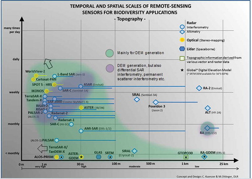
Table 5. “Topography”-related sensors.

Sensor name	Sensor type	Spatial resolution	Minimum local revisit time (days)	Maximum swath width (km)	Platform	Agency	Launch date
Topography
SRTM	Radar	90 m	-	Global coverage	Space Shuttle	NASA(NGA	2001
TerraSAR-X/ TanDEM-X	Radar	1–16 m (DEM 12 m)	11	10–100	TerraSAR-X/TanDem-X	DLR	2007/2011
Radarsat-1	Radar	8–100 m	24	20–500	Radarsat-1	CSA	1995
Radarsat-2	Radar	3–100 m	24	20–500	Radarsat-2	CSA	2007
WorldView-2	Optical	0.5–1.8 m	2.2–7.2d	16.4	WorldView-2	Digital Globe	2009
ASTER	Optical	30 m	16	60	Terra	NASA	1999
SPOT-HRS	Optical	5–10 m	4–6	120	SPOT 5	EADS Astrium	2002
IKONOS	Optical	1–4 m	6	11	IKONOS	GeoEye	1999
HRC (ZY-3)	Optical	3.5 m		52	ZY-3A	CRESDA	2012
PALSAR-2	Radar	1–100 m	14	25–350	ALOS-2	JAXA	2014
PALSAR	Radar	30 km/100 km	46	70–350	ALOS	JAXA	2006
ASAR	Radar	30–1000 m	2–7	5–405	Envisat	ESA	2002
PRISM	Optical	2.5 m	46/96 for stereoscopy	35–70	ALOS	NASDA	2006
CARTOSAT-PAN	Optical	1 m	4	10	CartoSat-2/2A/2B	ISRO	2007/2008/2010
SAR-C	Radar	5–80 m	12	80–400	Sentinel-1A	ESA	2014
SAR-S	Radar	5–25 m	4	40–100	HJ-1C	CRESDA	2012
GLAS	Lidar	66 m	91	Airborne	ICESAT	NASA	2003
AMI-SAR	Radar	30–1000 m	35	100	ERS-1/2	ESA	1991/1995
JERS-1 SAR	Radar	18 m	44	75	JERS-1	JAXA	1992
SAR-C	Radar	3–50 m	7–30	30–240	RISAT-1	ISRO	2012
SAR-X	Radar	3–8 m	5	10–650	RISAT-2	ISRO	2009
SEASAT	Radar	25 m	105	100	SEASAT-1	NASA	1978
RORSAT	Radar	n.a.	n.a.	n.a.	KOSMOS 102–1932	n.a.	1967–1988
Poseidon 3	Radar	30 km	10 days–1 month	30–100	Jason 2	NASA/NOAA/CNES/EUMETSAT	2008
SIRAL	Radar	250 m	369/30	15	Cryosat-2	ESA	2008
SRAL	Radar	300 m	10–30d	20	Sentinel-3A	ESA	2015
ALT	Radar	16 km	14	16	HY-2A	NSOAS, CAST	2011
RA	Radar	16–20 km	35	16–20	ERS-1/2	ESA	1991/1995
RA-2	Radar	10 km	2–7	10	Envisat	ESA	2002
SAR 2000	Radar	8 m	Global coverage in 14; (0.5 in full constellation)	10–200	Cosmo-SkyMed 1–4	ASI	2007/2008/2010
GTOPO 30	derived raster and vector sources	1 km	—	—	—	USGS	1996

SRTM, Shuttle Radar Topography Mapper; AMI-SAR, Active Microwave Instrumentation – Image Mode; ASTER, Advanced Spaceborne Thermal Emission and Reflection Radiometer; PR, Precipitation Radar; SPOT-HRS, SPOT- High-Resolution Stereoscope; SIRAL, SAR Interferometric Radar Altimeter; PALSAR, Phased Array type L-band Synthetic Aperture Radar; RA-2, Radar Altimeter-2; PRISM, Panchromatic Remote-Sensing Instrument for Stereo Mapping; PRSIM, Panchromatic Remote-Sensing Instrument for Stereo Mapping; Lidar, Light Detection and Ranging; AMI-SAR, Active Microwave Instrumentation – Image Mode.

All the radar sensors identified in Figure 10 also allow derivation of surface displacement based on differential SAR interferometry, DifInSAR. While in most places of the world such surface movement might not have a large impact on biodiversity, in some selected cases such data can be relevant. Sinking surfaces might indicate depleting water levels and thus less water available for plants. In the coastal zone, surface subsidence can lead to the submersion of land and changes in the coastal ecosystems. Sudden collapse of surfaces in karst, underground mining, or coal fire landscapes leads to the destruction of the ecosystem formerly covering the collapsed area. However, DifInSAR is definitely a niche-field in the remote sensing of biodiversity.

6. Data access and availability

The number of Earth observation sensors and the amount of archived remote-sensing data have steadily increased over the past decades. Figures 3 to 10 present the large fleet of optical, thermal, and radar sensors in orbit, suggesting that there is a huge amount of data available to the global community, including biologists, conservationists, and stakeholders.

However, data set access and availability is limited. Even for data sets that are available for download free of charge, it is often difficult for non-remote-sensing scientists or stakeholders to access them. Ways of data access are not known to everyone; many data sets are provided in crude formats; projections need to be adjusted, and many data sets require thorough pre-processing (sensor calibration, atmospheric correction, geocorrection/orthocorrection) before the data can be displayed as reflectance (%) or temperature (°C) values. There is no centralized global portal for downloading remote-sensing data, and depending on the data amount required (global coverage or extensive stacks of time series), it is also not possible for everyone to download and process the data (hardware restrictions, network speed restrictions, no programming skills). A large variety of data portals exist (e.g. earthexplorer.usgs.gov, landcover.org, glovis.usgs.org), but many are neither intuitive nor user friendly. Non-remote-sensing scientists can furthermore often not judge the quality of the provided data sets, as metadata, quality flag information, or even a crowd-sourcing-based rating (like for books in Amazon) is missing. Although some informative websites aim to provide insightful lists of available data download portals, they are usually not very comprehensive and far from exhaustive (e.g. remote-sensing-biodiversity.org/remote sensing/resources).

The main political and economic challenge to date is still to provide free and open access to remotely sensed data and products in order to support the application of such data for many different disciplines (Turner et al. 2013), including for the biodiversity and conservation community. The move of the USA towards open access to nearly all remote-sensing data collected from US platforms, and the future free and open access to ESA (Sentinels) as well as CNES data, will foster the use of remote sensing for biodiversity applications. This pathway should be continued in the future. Most remote-sensing sensors have been designed and even built in national research laboratories (in joint partnerships with industry) and have often been financed by taxpayers. A large part of remote-sensing science globally – no matter whether funding comes national governments, the World Bank, or other development banks – is also paid with taxpayers’ money. Therefore, the data, derived products, and knowledge gained therefrom should be made publicly available – in an easily accessible manner. This was also the call of Turner et al. (2013) in a short correspondence note to Nature titled: ‘Satellites: make data freely available’. However, oftentimes, the budgets are just large enough to launch a sensor into orbit, but maybe not to fund data storage or dissemination. Many space agencies and other institutions had the funding to launch a sensor – but were under-equipped to downlink, store, archive, preserve, and distribute the data – endeavours, whose costs can outweigh satellite design and launch costs by far. We simply cannot assume that – because an instrument was operating at a certain time – the data have automatically been kept and are available. The data may not have been collected, or it may have been received and not archived or it may have been archived but the data have become unreadable. However, costs of data storage, archiving, preservation, and dissemination should be considered, when sensor missions are evaluated for funding support.

Furthermore, sensor development has for many decades not exclusively been driven by the needs of scientific and ‘real-world’ decision-making users (although a ‘user requirements document’ can surely be presented by each space agency for each sensor development), and also not by global cooperation only. A strong emphasis has been national independence and the very reasonable desire to develop indigenous space technology (‘We are building our own optical/radar/thermal sensor so that we can be independent of others’ or ‘We should advance our space sector and industry’), national pride (‘There are already tens of optical sensors in orbit, but we will show the world that we can also do it’), a strong drive for ever improving technology (‘The data from sensor X has not even been fully exploited yet, however, since we are able to create a higher resolution satellite, let’s launch it into orbit’), and obstacles to cooperation between space nations (‘We cannot permit researchers from that country to attend our conferences or visit our labs’).

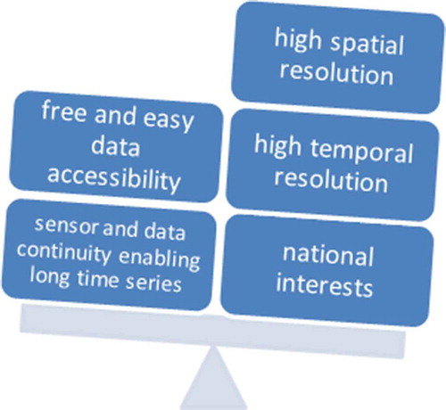
All these reasons, paired with shifts in the political leadership and priorities of countries and in decisions about how generous or restricted budgets are for space and Earth science activities, have led to the imbalance depicted in Figure 11; the former have been at the cost of, first, sensor and data continuity enabling long time series, and, second, free and easy data accessibility. This is reflected, for example, in delays in the launch of successor missions, which cause unfortunate data gaps that hinder needed research, and in duplication of efforts while other important fields are neglected.

Figure 11. Foci of sensor development and policy impacting data availability and continuity.

Of the more than 140 sensors reviewed for this article, only a few sensors exist which really allow continuous time-series monitoring exceeding 20 years, and only data from very few sensors are truly freely available (AVHRR, MODIS, MERIS, Landsat, Aster, ASAR, ATSR, AATSR, SCAT, ASCAT, Meteosat, and some others). Freely available we understand as being able to ‘open a website and download as much data as one likes, for as much spatial coverage as there is available’. Some sensor data are available in a ‘nearly freely available mode’. But to access this data, one has to write (sometimes short, sometimes lengthy) data proposals, fill out forms, and then be granted access to only a relatively small amount of data of the desired spatial or temporal coverage – so one cannot obtain as many data sets one needs to work with (for example, the very limited amount of TerraSAR-X, TanDEM-X, RapidEye, Radarsat, ALOS, TET, or SPOT data that can be accessed in practice). The reasons are: while possibly satisfactory for small individual studies or a master’s thesis, this situation is a nuisance for any remote-sensing scientist who aims for national, continental, or global coverage for his/her product or study, requires multiple data sources, and cannot understand why it is necessary to invest weeks and weeks in writing data proposals. Also, most data are only available at sometimes very high prices per square metre or scene (WorldView, QuickBird, IKONOS, Cartosat, GeoEye, Formosat, Radarsat). Much data cannot be purchased by the global community, but is only accessible to selected institutes or cooperation programmes. The unique and well-received European–Chinese Dragon Programme, coordinated by ESA and the National Remote Sensing Centre of China, is an example (access to selected Chinese sensor data sets, such as FY or CBERS, is allowed for European cooperation partners). Such situations may improve with time, when the benefits of cooperation are appreciated, and after crucial publications appear.

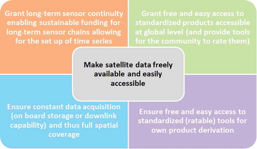
Although access to data from China, India, and other emerging global economies is still limited and the call for opening up the archives also applies to them, we should also understand that they do not want to share data with the global community that is not yet well calibrated, tested, and evaluated. It is illusory to assume that access to novel sensor data from emerging nations can be granted to the world within months after launch. After all, it also took the USA and Europe many years to open up their archives to the public. Emerging economies need to feel confident about the data they acquire before sharing them globally. Distributing badly calibrated or distorted sensor data would hold the potential of ‘face loss’ or professional criticism, and countries may not be able to have the infrastructure and administrative capacity in place to deal with global data requests. A good example has been given by the consortium around Gong et al. (2013) enabling access to global Landsat-derived land-cover data. Nevertheless, we consider the following appeal (Figure 12) worth making to data provider and remote-sensing community globally.

Figure 12. Appeal to governments, space agencies, and data providers.

The biodiversity community and conservationists – as well as most remote-sensing scientists – usually only tap the sensor data that are, first, easily accessible and mostly free of charge, and, second, have been sufficiently applied and described in literature, and, third, can be handled by a natural scientist without too much background in remote sensing. Complex data formats or unnecessarily complex demands of data pre-processing all hamper data spread and use. Currently, most biodiversity and conservation experts, who are not from the remote-sensing field, use data from sensors such as Landsat, MODIS, ASAR, or – if funds or support programmes are available – from high-resolution sensors such as IKONOS, QuickBird, GeoEye, WorldView, etc. Additionally, the convenience and influence of Google Earth should not be underestimated. In non-remote-sensing fields, it is quite common to work with single-band georectified screenshots from Google Earth, with manually digitized products derived on the basis of Google Earth products, and even with multitemporal information provided via this platform. Even within the remote-sensing field, Google Earth is nowadays often used for the collection of high-resolution sample points for training and indirect validation or the derivation of areal cover densities (Cracknell et al. 2013; Gong et al. 2013). Furthermore, most biologists, ecologists, and conservationists have a relatively local focus area or habitat of interest, and local studies based on a few Landsat scenes are often sufficient. Especially managers, decision-makers, and stakeholders cannot be expected to spend months with data pre-processing, and several months with data processing to finally obtain a highly scientific map, which the donors, politicians, and public authorities he/she addresses have trouble understanding.

An incredible value also lies in more complex time-series data sets, which can probably only be tapped by remote-sensing experts. Leyequien et al. (2007) underline the value of long-term data availability from sensors such as AVHRR and MODIS and believe that the ‘analysis of multiannual land-cover data potentially provides a key to understanding the influence of climate variability on shaping ecosystems – which form the overarching hierarchical layer in biodiversity assessment’.

Numerous biologists and conservationists are using species distribution models (SDMs) to predict the distribution of species as a function of environmental variables – and here especially climate variables (Cord et al. 2014). However, oftentimes the set of input variables is limited and information on terrain, land cover, land use, phenologic metrics, or proximities is not incorporated (Cord et al. 2014). However, with suitable sets of medium-resolution global data and derived products, it would be possible to create a global ‘Species Distribution Visualizer and Modeller based on Earth Observation Data’. Our idea is – in a simplified way – presented in Figure 13. The backbone of such a tool would be a database that contains all the ‘boundary conditions’ for selected species (describing the temperature, precipitation, and elevation ranges, and the land-cover/land-use and vegetation types usually associated with the species, and which proximity parameters such as maximum distances to coasts, lakes, etc. need to be ensured). Global time series of physical, index, thematic, topographic, and texture variables available for the past 30+ years and into the future would then allow past, present, and even future species extent to be modelled when considering future climate change or urban sprawl scenarios (see Figure 13). Our current judgment is that it will be data from sensors such as AVHRR and/or MODIS, supported by Landsat and the Sentinels, which will – in the long run – help to realize this idea.

Figure 13. Our concept of an ideal “Species Distribution Visualizer and Modeller” based on remote-sensing data. If a near unlimited number of daily globally available variables could be provided as time series up to 30–40 years back into the past (plus granting future continuity), it would be possible to model selected past, current, and possibly future habitats of animals or vegetation species after simply moving a slider to define the crucial variables. Of course, additional biodiversity data including GPS migration and tracking data, field data (ground truth), and further ancillary data would increase the value of such a tool.

In combination with a global database of biodiversity information (in situ abundance and species mapping, track data, etc.), such a tool would be of immeasurable value for a global overview – despite the fact that highly specific local or regional data will yield better results for the individual case. The biodiversity community makes very similar requests to the current remote-sensing community. Of course, the realization of this idea would require a large collaborative effort of remote-sensing scientists and biologists, ecologists, and conservationists alike. Technically, a realization is possible, but would depend on strong, cross-sectorial networks and sufficient funding.

7. Conclusion

Cross-sectorial dialogue between disciplines, such as the remote-sensing community and the community of biologists, ecologists, and conservationists, is essential for creating an improved understanding of each discipline’s assets and challenges. Biologists, ecologists, and conservationists are an important user group for information that can be derived from remote-sensing data. This group has an urgent need to map and quantify animal and vegetation biodiversity at local, national, regional, and global scales, considering different hierarchical levels of biodiversity at the species, habitat, and landscape levels. However, many knowledge gaps exist in both communities.

Remote-sensing experts might not be familiar with terms such as ‘taxa’, ‘invertebrates’, or ‘conservation gap analyses’. Biodiversity experts might not be aware of the many satellite sensors that exist and can be tapped for remote-sensing-based support of biodiversity-related mapping activities. Remote-sensing scientists might not know that habitat boundaries and land-cover classes do not always – or only rarely – correlate. Biodiversity experts might need to realize that much more information than just land cover or a vegetation index can be derived from remote-sensing data. Remote-sensing experts need to understand that managers and decision-makers from the field of biodiversity conservation need to be provided with maps and information products that can be understood by donors and public authorities, who might not be versed in the natural sciences. And the biodiversity community needs to provide information on habitat boundary conditions for animal and vegetation species whose habitats might be suitable for remote-sensing-based analysis.

To contribute to this dialogue and knowledge sharing, in this article we have provided an overview outlining how remote sensing has so far contributed to animal, vegetation, and habitat mapping, given a comprehensive overview of all currently existing optical, multispectral, thermal, and radar sensors in orbit, as well as the availability of long sensor lines, have presented details of the spatial and temporal resolutions of these sensors, as well as their most suitable fields of application with respect to biodiversity mapping, and elaborated on the complexities of data availability, access, and provision schemes. In general, the assessment of species biodiversity for animals is restricted, due to the non-stationary nature of most animals. To capture large animal herds with highest resolution satellite imagery is rather a product of chance, and cost efficient, reliable, and repeatable monitoring of animals themselves can hardly be undertaken. Individual animals are usually too small to be extracted from highest resolution data. The mapping of stationary vegetation species, which are often (but not always) defining an animal’s habitat, is easier and many more studies assess vegetation biodiversity from space than animal biodiversity. But even for vegetation species diversity assessments, remote sensing has limitations. Species that are much smaller than the spatial resolution of the sensor or that occur only scattered and alone-standing as well as species that exhibit similar reflectance characteristics as other species cannot be extracted or differentiated. For mapping requests at the local to site level, it has therefore to be taken into account that remote-sensing data might just provide a general outline, land-cover, and land-use information of the site, but that in situ mapping will yield cost-effective results at much higher quality.

This overview has furthermore elucidated the fact that it is however often also not sensor availability or spatial resolution that hinders us from providing the right data to the biodiversity community. A large variety of high-resolution optical, multispectral, and radar sensors exist. Currently, far over 100 imaging sensors are in orbit, all with their own spectral, spatial, and temporal characteristics and with spatial resolutions ranging from centimetres to kilometres, and with revisit times from two weeks up to several times per day.

A larger challenge than spatial resolution is temporal resolution – revisit time – and especially the available monitoring period: meaning, for how many years data of one sensor are available. For many sensors, data continuity is not given. Time series cannot be generated, multitemporal analyses only work for selected years, and intercomparability with products derived from other sensors is difficult. Also, maps generated once, with no capacity for updating, are problematic. We therefore consider long-term governmental support and programmes to ensure data continuity and stable sensor lines to be the most pressing need.

Next to long-term continuity, the major bottleneck is obtaining access to Earth observation data. It is a great asset that many US and European data providers have opened up their archives and that nowadays data sets from many important sensors are available free of charge. However, much data of high value for the biodiversity community only come at a high cost or are of very limited availability, as global monitoring is not ensured. It has been underlined by numerous authors (Nagendra et al. 2013; Leyequien et al. 2007) that it is especially the available choice of data that will determine the type of information that can be derived for mapping complex, fine-scale, and structurally variable habitats to the degree of accuracy sought by stakeholders and decision-makers. Facing the urgent need to monitor our planet, we would hurt ourselves if not all emphasis is put on making sensor data rapidly available in a free and effective manner. We therefore underline recent calls such as that of Turner et al. (2013) to make satellite data freely available.

Last but not least, we currently see large chances for cooperation between the biodiversity and remote-sensing communities in the field of direct, or proxy-driven time-series analysis of habitats and habitat changes. Regional or even global time series of physical, index, thematic, topographic, and texture variables – if analysed jointly – can support long-term understanding of climate change- and human-induced habitat shifts and losses. When combined with knowledge of species boundary conditions, as well as with a global collection of in situ biodiversity data and tracking data, this approach could tap a wealth of new information.

References

- Abraham, C. 2014. “Rhino Horn is Not Medicine.” New Scientist 222 (2966): 27. doi:10.1016/S0262-4079(14)60828-9.
- Bai, Y., N. Walsworth, B. Roddan, D. A. Hill, K. Broersma, and D. Thompson. 2005. “Quantifying Tree Cover in the Forest–Grassland Ecotone of British Columbia Using Crown Delineation and Pattern Detection.” Forest Ecology and Management 212 (1–3): 92–100. doi:10.1016/j.foreco.2005.03.005.
- Baker, A. C., P. W. Glynn, and B. Riegl. 2008. “Climate Change and Coral Reef Bleaching: An Ecological Assessment of Long-Term Impacts, Recovery Trends and Future Outlook.” Estuarine Coastal and Shelf Science 80 (4): 435–471. doi:10.1016/j.ecss.2008.09.003.
- Baret, F., and G. Guyot. 1991. “Potentials and Limits of Vegetation Indices for LAI and APAR Assessment.” Remote Sensing of Environment 35 (2–3): 161–173. doi:10.1016/0034-4257(91)90009-U.
- Barnosky, A. D., N. Matzke, S. Tomiya, G. O. U. Wogan, B. Swartz, T. B. Quental, C. Marshall, J. L. McGuire, E. L. Lindsey, K. C. Maguire, B. Mersey, and E. A. Ferrer. 2011. “Has the Earth’s Sixth Mass Extinction Already Arrived?” Nature 471: 51–57. doi:10.1038/nature09678.
- Belluco, E., M. Camuffo, S. Ferrari, L. Modenese, S. Silvestri, A. Marani, and M. Marani. 2006. “Mapping Salt-marsh Vegetation by Multispectral and Hyperspectral Remote Sensing.” Remote Sensing of Environment 105 (1): 54–67.
- Benali, A., J. P. Nunes, F. B. Freitas, C. A. Sousa, M. T. Novo, P. M. Lourenço, J. C. Lima, J. Seixas, and A. P. G. Almeida. 2014. “Satellite-Derived Estimation of Environmental Suitability for Malaria Vector Development in Portugal.” Remote Sensing of Environment 145: 116–130. doi:10.1016/j.rse.2014.01.014.
- Biggs, R., H. Simons, M. Bakkenes, R. J. Scholes, B. Eickhout, D. Van Vuuren, and R. Alkemade. 2008. “Scenarios of Biodiversity Loss in Southern Africa in the 21st Century.” Global Environmental Change 18 (2): 296–309. doi:10.1016/j.gloenvcha.2008.02.001.
- Birnie, R. V., R. A. Robertson, and G. C. Stove. 1982. “Remote Sensing for Agricultural Research and Monitoring Operations.” Agriculture and Environment 7 (2): 121–134. doi:10.1016/0304-1131(82)90002-9.
- Blasco, F., T. Gauquelin, M. Rasolofoharinoro, J. Denis, M. Aizpuru, and V. Caldairou. 1998. “Recent Advances in Mangrove Studies Using Remote Sensing.” Marine and Freshwater Research 49 (4): 287–296. doi:10.1071/MF97153.
- Blondeau-Patissier, D., J. F. R. Gower, A. G. Dekker, S. R. Phinn, and V. E. Brando. 2014. “A Review of Ocean Color Remote Sensing Methods and Statistical Techniques for the Detection, Mapping and Analysis of Phytoplankton Blooms in Coastal and Open Oceans.” Progress in Oceanography 123: 123–144. doi:10.1016/j.pocean.2013.12.008.
- Brakke, T. W., E. T. Kanemasu, J. L. Steiner, F. T. Ulaby, and E. Wilson. 1981. “Microwave Radar Response to Canopy Moisture, Leaf-Area Index, and Dry Weight of Wheat, Corn, and Sorghum.” Remote Sensing of Environment 11: 207–220. doi:10.1016/0034-4257(81)90020-1.
- Brand, U., R. Posenato, R. Came, H. Affek, L. Angiolini, K. Azmy, and E. Farabegoli. 2012. “The End‐Permian Mass Extinction: A Rapid Volcanic CO2 and CH4‐Climatic Catastrophe.” Chemical Geology 322–323: 121–144. doi:10.1016/j.chemgeo.2012.06.015.
- Briant, G., V. Gond, and S. W. G. Laurance. 2010. “Habitat Fragmentation and the Desiccation of Forest Canopies: A Case Study from Eastern Amazonia.” Biological Conservation 143 (11): 2763–2769. doi:10.1016/j.biocon.2010.07.024.
- Brown, D. D., S. Lapoint, R. Kays, W. Heidrich, F. Kümmeth, and M. Wikelski. 2012. “Accelerometer-Informed GPS Telemetry: Reducing the Trade-Off between Resolution and Longevity.” Wildlife Society Bulletin 36 (1): 139–146. doi:10.1002/wsb.111.
- Buerkert, A., and E. Schlecht. 2009. “Performance of Three GPS Collars to Monitor Goats’ Grazing Itineraries on Mountain Pastures.” Computers and Electronics in Agriculture 65: 85–92. doi:10.1016/j.compag.2008.07.010.
- Burton, M. 1999. “An Assessment of Alternative Methods of Estimating the Effect of the Ivory Trade Ban on Poaching Effort.” Ecological Economics 30 (1): 93–106. doi:10.1016/S0921-8009(98)00102-5.
- Casa, R., and H. G. Jones. 2005. “LAI Retrieval from Multiangular Image Classification and Inversion of a Ray Tracing Model.” Remote Sensing of Environment 98 (4): 414–428. doi:10.1016/j.rse.2005.08.005.
- Chuang, T.-W., G. M. Henebry, J. S. Kimball, D. L. Vanroekel-Patton, M. B. Hildreth, and M. C. Wimberly. 2012. “Satellite Microwave Remote Sensing for Environmental Modeling of Mosquito Population Dynamics.” Remote Sensing of Environment 125: 147–156. doi:10.1016/j.rse.2012.07.018.
- Cooke, S. J., S. G. Hinch, M. Wikelski, R. D. Andrews, L. J. Kuchel, T. G. Wolcott, and P. J. Butler. 2004. “Biotelemetry: A Mechanistic Approach to Ecology.” Trends in Ecology & Evolution 19 (6): 334–343. doi:10.1016/j.tree.2004.04.003.
- Cord, A. F., D. Klein, F. Mora, and S. Dech. 2014. “Comparing the Suitability of Classified Land Cover Data and Remote Sensing Variables for Modeling Distribution Patterns of Plants.” Ecological Modelling 272: 129–140. doi:10.1016/j.ecolmodel.2013.09.011.
- Costello, M. J., W. K. Michener, M. Gahegan, Z.-Q. Zhang, and P. E. Bourne. 2013. “Biodiversity Data Should be Published, Cited, and Peer Reviewed.” Trends in Ecology & Evolution 28 (8): 454–461. doi:10.1016/j.tree.2013.05.002.
- Costello, M. J., and J. Wieczorek. 2014. “Best Practice for Biodiversity Data Management and Publication.” Biological Conservation 173: 68–73. doi:10.1016/j.biocon.2013.10.018.
- Cracknell, A. P. 1997. The Advanced Very High Resolution Radiometer (AVHRR). 534 pp. London: Taylor & Francis. ISBN 0 7484 0209 8.
- Cracknell, A. P. 2010. “Surrey Satellite Technology Limited (SSTL) and the Disaster Monitoring Constellation (DMC).” In Small Satellites for Earth Observation, edited by R. Sandau, H.-P. Röser, and A. Valenzuelo, 455 pp. Netherlands: Springer. http://www.springer.com/new+%26+forthcoming+titles+(default)/book/978-1-4020-6942-0
- Cracknell, A. P., K. D. Kanniah, K. P. Tan, and L. Wang. 2013. “Evaluation of MODIS Gross Primary Productivity and Land Cover Products for the Humid Tropics Using Oil Palm Trees in Peninsular Malaysia and Google Earth Imagery.” International Journal of Remote Sensing 34 (20): 7400–7423. doi:10.1080/01431161.2013.820367.
- Dell, A. I., J. A. Bender, K. Branson, I. D. Couzin, G. G. De Polavieja, L. P. J. J. Noldus, A. Pérez-Escudero, P. Perona, A. D. Straw, M. Wikelski, and U. Brose. 2014. “Automated Image-Based Tracking and Its Application in Ecology.” Trends in Ecology & Evolution 29 (7): 417–428. doi:10.1016/j.tree.2014.05.004.
- Dietz, A. 2013. “Central Asian Snow Cover Characteristics between 1986 and 2012 derived from Time Series of Medium Resolution Remote Sensing Data.” Dissertation, University of Wuerzburg, 208 pp.
- Duncan, C., D. Kretz, M. Wegmann, T. Rabeil, and N. Pettorelli. 2014. “Oil in the Sahara: Mapping Anthropogenic Threats to Saharan Biodiversity from Space.” Philosophical Transactions of the Royal Society B: Biological Sciences 369: 20130191. doi:10.1098/rstb.2013.0191.
- Eisfelder, C., C. Kuenzer, and S. Dech. 2011. “Derivation of Biomass Information for Semi-Arid Areas Using Remote-Sensing Data.” International Journal of Remote Sensing. doi:10.1080/01431161.2011.620034.
- Engler, R., L. T. Waser, N. E. Zimmermann, M. Schaub, S. Berdos, C. Ginzler, and A. Psomas. 2013. “Combining Ensemble Modeling and Remote Sensing for Mapping Individual Tree Species at High Spatial Resolution.” Forest Ecology and Management 310: 64–73. doi:10.1016/j.foreco.2013.07.059.
- Esch, T., M. Thiel, A. Schenk, A. Roth, A. Muller, and S. Dech. 2010. “Delineation of Urban Footprints from TerraSAR-X Data by Analyzing Speckle Characteristics and Intensity Information.” IEEE Transactions on Geoscience and Remote Sensing 48 (2): 905–916. doi:10.1109/TGRS.2009.2037144.
- Fensholt, R., I. Sandholt, and M. S. Rasmussen. 2004. “Evaluation of MODIS LAI, fAPAR and the Relation between fAPAR and NDVI in a Semi-Arid Environment Using in Situ Measurements.” Remote Sensing of Environment 91 (3–4): 490–507. doi:10.1016/j.rse.2004.04.009.
- Fingas, M., and C. Brown. 2014. “Review of Oil Spill Remote Sensing.” Marine Pollution Bulletin 83 (1): 9–23. doi:10.1016/j.marpolbul.2014.03.059.
- Flaspohler, D. J., C. P. Giardina, G. P. Asner, P. Hart, J. Price, C. K. Lyons, and X. Castaneda. 2010. “Long-Term Effects of Fragmentation and Fragment Properties on Bird Species Richness in Hawaiian Forests.” Biological Conservation 143 (2): 280–288. doi:10.1016/j.biocon.2009.10.009.
- Foody, G. M., and M. E. J. Cutler. 2006. “Mapping the Species Richness and Composition of Tropical Forests from Remotely Sensed Data with Neural Networks.” Ecological Modelling 195 (1–2): 37–42. doi:10.1016/j.ecolmodel.2005.11.007.
- Fretwell, P. T., I. J. Staniland, and J. Forcada. 2014. “Whales from Space: Counting Southern Right Whales by Satellite.” PLoS ONE 9 (2): 1–9. doi:10.1371/journal.pone.0088655.
- Fretwell, P. T., and P. N. Trathan. 2009. “Penguins from Space: Faecal Stains Reveal the Location of Emperor Penguin Colonies.” Global Ecology and Biogeography 18: 543–552. doi:10.1111/j.1466-8238.2009.00467.x.
- Fuller, R. M., G. B. Groom, S. Mugisha, P. Ipulet, D. Pomeroy, A. Katende, R. Bailey, and R. Ogutu-Ohwayo. 1998. “The Integration of Field Survey and Remote Sensing for Biodiversity Assessment: A Case Study in the Tropical Forests and Wetlands of Sango Bay, Uganda.” Biological Conservation 86 (3): 379–391. doi:10.1016/S0006-3207(98)00005-6.
- Gardner, T. A., N. D. Burgess, N. Aguilar-Amuchastegui, J. Barlow, E. Berenguer, T. Clements, F. Danielsen, J. Ferreira, W. Foden, V. Kapos, S. M. Khan, A. C. Lees, L. Parry, R. M. Roman-Cuesta, C. B. Schmitt, N. Strange, I. Theilade, and I. C. G. Vieira. 2012. “A Framework for Integrating Biodiversity Concerns into National REDD+ Programmes.” Biological Conservation 154: 61–71. doi:10.1016/j.biocon.2011.11.018.
- Gaston, K. J. 2000. “Global Patterns in Biodiversity.” Nature 405: 220–227. doi:10.1038/35012228.
- Gillespie, T. W., J. Chu, E. Frankenberg, and D. Thomas. 2007. “Assessment and Prediction of Natural Hazards from Satellite Imagery.” Progress in Physical Geography 31 (5): 459–470. doi:10.1177/0309133307083296.
- Goetz, A. F. H. 2009. “Three Decades of Hyperspectral Remote Sensing of the Earth: A Personal View.” Remote Sensing of Environment 113: S5–16. doi:10.1016/j.rse.2007.12.014.
- Gong, P., J. Wang, L. Yu, Y. Zhao, Y. Zhao, L. Liang, Z. Niu, X. Huang, H. Fu, S. Liu, C. Li, X. Li, W. Fu, C. Liu, Y. Xu, X. Wang, Q. U. Cheng, L. Hu, W. Yao, H. Zhang, P. Zhu, Z. Zhao, H. Zhang, Y. Zheng, L. Ji, Y. Zhang, H. Chen, A. N. Yan, J. Guo, L. Yu, L. Wang, X. Liu, T. Shi, M. Zhu, Y. Chen, G. Yang, P. Tang, B. Xu, C. Giri, N. Clinton, Z. Zhu, J. Chen, and J. Chen. 2013. “Finer Resolution Observation and Monitoring of Global Land Cover: First Mapping Results with Landsat TM and ETM+ Data.” International Journal of Remote Sensing 34 (7): 2607–2654. doi:10.1080/01431161.2012.748992.
- Gould, W. 2000. “Remote Sensing of Vegetation, Plant Species Richness, and Regional Biodiversity Hotspots.” Ecological Applications 10 (6): 1861–1870. doi:10.1890/1051-0761(2000)010[1861:RSOVPS]2.0.CO;2.
- Griffiths, G. H., J. Lee, and B. C. Eversham. 2000. “Landscape Pattern and Species Richness; Regional Scale Analysis from Remote Sensing.” International Journal of Remote Sensing 21 (13–14): 2685–2704. doi:10.1080/01431160050110232.
- Groom, G., M. Stjernholm, R. D. Nielsen, A. Fleetwood, and I. K. Petersen. 2013. “Remote Sensing Image Data and Automated Analysis to Describe Marine Bird Distributions and Abundances.” Ecological Informatics 2–8. doi:10.1016/j.ecoinf.2012.12.001.
- Gupta, R. K. 1993. “NOAA/AVHRR Vegetation Indices as Agrometeorological Growth Parameter.” Advances in Space Research 13 (5): 223–232. doi:10.1016/0273-1177(93)90549-Q.
- Gupta, R. K., T. S. Prasad, and D. Vijayan. 2000. “Relationship between LAI and NDVI for IRS LISS and Landsat TM Bands.” Advances in Space Research 26 (7): 1047–1050. doi:10.1016/S0273-1177(99)01115-1.
- Hansen, M. C., P. V. Potapov, R. Moore, M. Hancher, S. A. Turubanova1, A. Tyukavina, D. Thau, S. V. Stehman, S. Goetz, T. R. Loveland, A. Kommareddy, A. Egorov, L. Chini, C. O. Justice, and J. R. G. Townshend. 2013. “High-Resolution Global Maps of 21st-Century Forest Cover Change.” Science 342 (6160): 850–853. doi:10.1126/science.1244693.
- Hatfield, J. L. 1983. “Remote Sensing Estimators of Potential and Actual Crop Yield.” Remote Sensing of Environment 13 (4): 301–311. doi:10.1016/0034-4257(83)90032-9.
- Hay, S. I., R. W. Snow, and D. J. Rogers. 1998. “Predicting Malaria Seasons in Kenya Using Multitemporal Meteorological Satellite Sensor Data.” Transactions of the Royal Society of Tropical Medicine and Hygiene 92 (1): 12–20. doi:10.1016/S0035-9203(98)90936-1.
- Hazen, H. 2009. “Biodiversity Mapping.” In International Encyclopedia of Human Geography, edited by R. Kitchin and N. Thrift, 314–319. Oxford: Elsevier. doi:10.1016/B978-008044910-4.00006-7.
- Henderson, F. M., and A. J. Lewis. 2008. “Radar Detection of Wetland Ecosystems: A Review.” International Journal of Remote Sensing 29 (20): 5809–5835. doi:10.1080/01431160801958405.
- Herbreteau, V., G. Salem, M. Souris, J.-P. Hugot, and J.-P. Gonzalez. 2007. “Thirty Years of Use and Improvement of Remote Sensing, Applied to Epidemiology: From Early Promises to Lasting Frustration.” Health & Place 13 (2): 400–403. doi:10.1016/j.healthplace.2006.03.003.
- Hese, S., W. Lucht, C. Schmullius, M. Barnsley, R. Dubayah, D. Knorr, K. Neumann, T. Riedel, and K. Schröter. 2005. “Global Biomass Mapping for an Improved Understanding of the CO2 Balance—The Earth Observation Mission Carbon-3D.” Remote Sensing of Environment 94 (1): 94–104. doi:10.1016/j.rse.2004.09.006.
- Hirano, A., R. Welch, and H. Lang. 2003. “Mapping from ASTER Stereo Image Data: DEM Validation and Accuracy Assessment.” ISPRS Journal of Photogrammetry and Remote Sensing 57 (5–6): 356–370. doi:10.1016/S0924-2716(02)00164-8.
- Hoepffner, N., and G. Zibordi. 2009. “Remote Sensing of Coastal Waters.” In Encyclopedia of Ocean Sciences, edited by J. H. Steele, 2nd ed., 732–741. Oxford: Academic Press. doi:10.1016/B978-012374473-9.00801-8.
- Horie, T., M. Yajima, and H. Nakagawa. 1992. “Yield Forecasting.” Agricultural Systems 40 (1–3): 211–236. doi:10.1016/0308-521X(92)90022-G.
- Huete, A., Q. H. Liu, K. Batchily, and W. V. Leeuwen. 1997. “A Comparison of Vegetation Indices over a Global Set of TM Images for EOS-MODIS.” Remote Sensing of Environment 59: 440–451. doi:10.1016/S0034-4257(96)00112-5.
- Hughes, G. R., P. Luschi, R. Mencacci, and F. Papi. 1998. “The 7000-km Oceanic Journey of a Leatherback Turtle Tracked by Satellite.” Journal of Experimental Marine Biology and Ecology 229: 209–217. doi:10.1016/S0022-0981(98)00052-5.
- Irons, J. R., J. L. Dwyer, and J. A. Barsi. 2012. “The Next Landsat Satellite: The Landsat Data Continuity Mission.” Remote Sensing of Environment 122: 11–21. doi:10.1016/j.rse.2011.08.026.
- Jackson, R. D., and A. R. Huete. 1991. “Interpreting Vegetation Indices.” Preventive Veterinary Medicine 11 (3–4): 185–200. doi:10.1016/S0167-5877(05)80004-2.
- Jonsson, T., P. Karlsson, and A. Jonsson. 2006. “Food Web Structure Affects the Extinction Risk of Species in Ecological Communities.” Ecological Modelling 199: 93–106. doi:10.1016/j.ecolmodel.2006.06.012.
- Justice, C. O. 1992. “Satellite Monitoring of Tropical Forests. A Commentary on Current Status and International Roles. In Proceedings of the World Forest Watch Conference CEC EUR 14651 EN, edited by J.-P. Malingreau, R. Da Cunha, and C. Justice. Ispra: Joint Research Centre, CEC.
- Kachelriess, D., M. Wegmann, M. Gollock, and N. Pettorelli. 2014. “The Application of Remote Sensing for Marine Protected Area Management.” Ecological Indicators 36: 169–177. doi:10.1016/j.ecolind.2013.07.003.
- Karlsson, P., T. Jonsson, and A. Jonsson. 2007. “Food Web Structure and Interaction Strength Pave the Way for Vulnerability to Extinction.” Journal of Theoretical Biology 249: 77–92. doi: 10.1016/j.jtbi.2007.07.013.
- Kataoka, R., T. Ebisuzaki, H. Miyahara, T. Nimura, T. Tomida, T. Sato, and S. Maruyama. 2014. “The Nebula Winter: The United View of the Snowball Earth, Mass Extinctions, and Explosive Evolution in the Late Neoproterozoic and Cambrian Periods.” Gondwana Research 25: 1153–1163. doi:10.1016/j.gr.2013.05.003.
- Kivinen, S., and T. Kumpula. 2014. “Detecting Land Cover Disturbances in the Lappi Reindeer Herding District Using Multi-Source Remote Sensing and GIS Data.” International Journal of Applied Earth Observation and Geoinformation 27 (A): 13–19. doi:10.1016/j.jag.2013.05.009.
- Klemas, V. 2013. “Fisheries Applications of Remote Sensing: An Overview.” Fisheries Research 148: 124–136. doi:10.1016/j.fishres.2012.02.027.
- Knauer, K., U. Gessner, S. Dech, and C. Kuenzer. 2014. “Remote Sensing of Vegetation Dynamics in West Africa.” International Journal of Remote Sensing. doi:10.1080/01431161.2014.954062.
- Knudsen, E., A. Lindén, C. Both, N. Jonzén, F. Pulido, N. Saino, W. J. Sutherland, L. A. Bach, T. Coppack, T. Ergon, P. Gienapp, J. A. Gill, O. Gordo, A. Hedenström, E. Lehikoinen, P. P. Marra, A. P. Møller, A. L. K. Nilsson, G. Péron, E. Ranta, D. Rubolini, T. H. Sparks, F. Spina, C. E. Studds, S. A. Saether, P. Tryjanowski, and N. C. Stenseth. 2011. “Challenging Claims in the Study of Migratory Birds and Climate Change.” Biological Reviews 86 (4): 928–946. doi:10.1111/j.1469-185X.2011.00179.x.
- Kramer, H. 2002. Observation of the Earth and Its Environment: Survey of Missions and Sensors, 3rd ed. Springer Science & Business Media. http://www.springer.com/engineering/mechanical+engineering/book/978-3-642-62688-3
- Kranstauber, B., A. Cameron, R. Weinzerl, T. Fountain, S. Tilak, M. Wikelski, and R. Kays. 2011. “The Movebank Data Model for Animal Tracking.” Environmental Modelling & Software 26 (6): 834–835. doi:10.1016/j.envsoft.2010.12.005.
- Kuemmerle, T., K. Perzanowski, O. Chaskovskyy, K. Ostapowicz, L. Halada, A.-T. Bashta, I. Kruhlov, P. Hostert, D. M. Waller, and V. C. Radeloff. 2010. “European Bison habitat in the Carpathian Mountains.” Biological Conservation 143 (4): 908–916. doi:10.1016/j.biocon.2009.12.038.
- Kuenzer, C., A. Bluemel, S. Gebhardt, T. V. Quoc, and S. Dech. 2011. “Remote Sensing of Mangrove Ecosystems: A Review.” Remote Sensing 3: 878–928. doi:10.3390/rs3050878.
- Kuenzer, C., and S. Dech. 2013. “Theoretical Background of Thermal Infrared Remote Sensing.” In Thermal Infrared Remote Sensing – Sensors, Methods, Applications. Remote Sensing and Digital Image Processing Series, Vol. 17, edited by C. Kuenzer and S. Dech. 572 pp. Dordrecht: Springer Science+Business Media. ISBN 978-94-007-6638-9, pp-1-26.
- Kuenzer, C., C. Hecker, J. Zhang, S. Wessling, and W. Wagner. 2008. “The Potential of Multidiurnal MODIS Thermal Band Data for Coal Fire Detection.” International Journal of Remote Sensing 29: 923–944. doi:10.1080/01431160701352147.
- Kuenzer, C., and K. Knauer. 2013. “Remote Sensing of Rice Crop Areas.” International Journal of Remote Sensing 34 (6): 2101–2139. doi:10.1080/01431161.2012.738946.
- Kutser, T., and D. L. B. Jupp. 2006. “On the Possibility of Mapping Living Corals to the Species Level Based on Their Optical Signatures.” Estuarine Coastal and Shelf Science 69 (3–4): 607–614. doi:10.1016/j.ecss.2006.05.026.
- Lawler, S. P. 2001. “Rice Fields as Temporary Wetlands: A Review.” Israel, Journal of Zoology 47 (4): 513–528. doi:10.1560/X7K3-9JG8-MH2J-XGX1.
- Legović, T., J. Klanjšček, and S. Geček. 2010. “Maximum Sustainable Yield and Species Extinction in Ecosystems.” Ecological Modelling 221: 1569–1574. doi:10.1016/j.ecolmodel.2010.03.024.
- Leifer, I., W. J. Lehr, D. Simecek-Beatty, E. Bradley, R. Clark, P. Dennison, Y. Hu, S. Matheson, C. E. Jones, B. Holt, M. Reif, D. A. Roberts, J. Svejkovsky, G. Swayze, and J. Wozencraft. 2012. “State of the Art Satellite and Airborne Marine Oil Spill Remote Sensing: Application to the BP Deepwater Horizon Oil Spill.” Remote Sensing of Environment 124: 185–209. doi:10.1016/j.rse.2012.03.024.
- Leinenkugel, P., M. Wolters, C. Kuenzer, N. Oppelt, and S. Dech. 2014. “Sensitivity Analysis for Predicting Continuous Fields of Tree-Cover and Fractional Land-Cover Distributions in Cloud-Prone Areas.” International Journal of Remote Sensing 35 (8): 2799–2821. doi:10.1080/01431161.2014.890302.
- Leinenkugel, P., M. Wolters, N. Oppelt, and C. Kuenzer. Forthcoming. “Tree Cover and Forest Cover Dynamics in the Mekong Basin from 2001 to 2011.” Remote Sensing of Environment.
- Leyequien, E., J. Verrelst, M. Slot, G. Schaepman-Strub, I. M. A. Heitkönig, and A. Skidmore. 2007. “Capturing the Fugitive: Applying Remote Sensing to Terrestrial Animal Distribution and Diversity.” International Journal of Applied Earth Observation and Geoinformation 9 (1): 1–20. doi:10.1016/j.jag.2006.08.002.
- Löffler, E., and C. Margules. 1980. “Wombats Detected from Space.” Remote Sensing of Environment 9: 47–56. doi:10.1016/0034-4257(80)90046-2.
- Loveland, T. R., and J. L. Dwyer. 2012. “Landsat: Building a Strong Future.” Remote Sensing of Environment 122: 22–29. doi:10.1016/j.rse.2011.09.022.
- Lu, D. 2006. “The Potential and Challenge of Remote Sensing‐Based Biomass Estimation.” International Journal of Remote Sensing 27 (7): 1297–1328. doi:10.1080/01431160500486732.
- Malingreau, J.-P. 1992. “Satellite-Based Forest Monitoring. A Review of Current Issues.” In Proceedings of the World Forest Watch Conference. CEC EUR 14651 EN, edited by J.-P. Malingreau, R. Da Cunha, and C. Justice. Ispra: Joint Research Centre, CEC.
- Melesse, A. M., Q. Weng, P. S. Thenkabail, and G. B. Senay. 2007. “Remote Sensing Sensors and Applications in Environmental Resources Mapping and Modelling.” Sensors 7 (12): 3209–3241. doi:10.3390/s7123209.
- Murwira, A., A. K. Skidmore, H. J. G. Huizing, and H. H. T. Prins. 2010. “Remote Sensing of the Link between Arable Field and Elephant (Loxodonta africana) Distribution Change along a Tsetse Eradication Gradient in the Zambezi Valley, Zimbabwe.” International Journal of Applied Earth Observation and Geoinformation 12 (1): S123–S130. doi:10.1016/j.jag.2009.09.007.
- Myers, N., R. A. Mittermeier, C. G. Mittermeier, G. A. F. Da Fonseca, and J. Kent. 2000. “Biodiversity Hotspots for Conservation Priorities.” Nature 403: 853–858. doi:10.1038/35002501.
- Nagendra, H. 2001. “Using Remote Sensing to Assess Biodiversity.” International Journal of Remote Sensing 22 (12): 2377–2400. doi:10.1080/01431160117096.
- Nagendra, H., R. Lucas, J. P. Honrado, R. H. G. Jongman, C. Tarantino, M. Adamo, and P. Mairota. 2013. “Remote Sensing for Conservation Monitoring: Assessing Protected Areas, Habitat Extent, Habitat Condition, Species Diversity, and Threats.” Ecological Indicators 33: 45–59. doi:10.1016/j.ecolind.2012.09.014.
- Nellis, M. D., and C. E. Bussing. 1990. “Spatial Variation in Elephant Impact on the Zambezi Teak Forest in the Chobe National Park, Botswana.” Geocarto International 5: 55–57. doi:10.1080/10106049009354259.
- O’dor, R. K., K. Fennel, and E. Berghe. 2009. “A One Ocean Model of Biodiversity.” Deep Sea Research Particle II: Topical Studies in Oceanography 56 (19–20): 1816–1823. doi:10.1016/j.dsr2.2009.05.023.
- Olson, D., E. Dinerstein, E. D. Wikramanayake, N. D. Burgess, G. V. N. Powell, E. C. Underwood, J. A. D’amico, I. Itoua, H. E. Strand, J. C. Morrison, C. J. Loucks, T. F. Allnutt, T. H. Ricketts, Y. Kura, J. F. Lamoreux, W. W. Wettengel, P. Hedao, and K. R. Kassem. 2001. “Terrestrial Ecoregions of the World: A New Map of Life on Earth.” Bioscience 51: 933–938. doi:10.1641/0006-3568(2001)051[0933:TEOTWA]2.0.CO;2.
- Papi, F., M. Apollonio, B. Vaschetti, and S. Benvenuti. 1997. “Satellite tracking of a White Stork from Italy to Morocco.” Behavioural Processes 39: 291–294. doi:10.1016/S0376-6357(96)00752-8.
- Pereira, H. M., S. Ferrier, M. Walters, G. N. Geller, R. H. G. Jongman, R. J. Scholes, M. W. Bruford, N. Brummitt, S. H. M. Butchart, A. C. Cardoso, N. C. Coops, E. Dulloo, D. P. Faith, J. Freyhof, R. D. Gregory, C. Heip, R. Höft, G. Hurtt, W. Jetz, D. S. Karp, M. A. McGeoch, D. Obura, Y. Onoda, N. Pettorelli, B. Reyers, R. Sayre, J. P. W. Scharlemann, S. N. Stuart, E. Turak, M. Walpole, and M. Wegmann. 2013. “Essential Biodiversity Variables.” Science 18 (339): 277–278.
- Pino-Del-Carpio, A., A. H. Ariño, A. Villarroya, J. Puig, and R. Miranda. 2014. “The Biodiversity Data Knowledge Gap: Assessing Information Loss in the Management of Biosphere Reserves.” Biological Conservation 173: 74–79. doi:10.1016/j.biocon.2013.11.020.
- Potapov, P. V., S. A. Turubanova, M. C. Hansen, B. Adusei, M. Broich, A. Altstatt, L. Mane, and C. O. Justice. 2012. “Quantifying Forest Cover Loss in Democratic Republic of the Congo, 2000–2010, with Landsat ETM+ Data.” Remote Sensing of Environment 122: 106–116. doi:10.1016/j.rse.2011.08.027.
- Priede, I. G., and J. French. 1991. “Tracking of Marine Animals by Satellite.” International Journal of Remote Sensing 12 (4): 667–680. doi:10.1080/01431169108929684.
- Pu, R., and S. Landry. 2012. “A Comparative Analysis of High Spatial Resolution IKONOS and Worldview-2 Imagery for Mapping Urban Tree Species.” Remote Sensing of Environment 124: 516–533. doi:10.1016/j.rse.2012.06.011.
- Pueyo, Y., and C. L. Alados. 2007. “Effects of Fragmentation, Abiotic Factors and Land Use on Vegetation Recovery in a Semi-Arid Mediterranean Area.” Basic and Applied Ecology 8 (2): 158–170. doi:10.1016/j.baae.2006.03.009.
- Raizman, E. A., H. B. Rasmussen, L. E. King, F. W. Ihwagi, and I. Douglas-Hamilton. 2013. “Feasibility Study on the Spatial and Temporal Movement of Samburu’s Cattle and Wildlife in Kenya Using GPS Radio-Tracking, Remote Sensing and GIS.” Preventive Veterinary Medicine 111 (1–2): 76–80. doi:10.1016/j.prevetmed.2013.04.007.
- Röder, A., T. H. Udelhoven, J. Hill, G. Del Barrio, and G. Tsiourlis. 2008. “Trend Analysis of Landsat-TM and -ETM+ Imagery to Monitor Grazing Impact in a Rangeland Ecosystem in Northern Greece.” Remote Sensing of Environment 112 (6): 2863–2875. doi:10.1016/j.rse.2008.01.018.
- Rundquist, D. C., S. Narumalani, and R. M. Narayanan. 2001. “A Review of Wetlands Remote Sensing and Defining New Considerations.” Remote Sensing Reviews 20 (3): 207–226. doi: 10.1080/02757250109532435.
- Saatchi, S., W. Buermann, H. Ter Steege, S. Mori, and T. B. Smith. 2008. “Modeling Distribution of Amazonian Tree Species and Diversity Using Remote Sensing Measurements.” Remote Sensing of Environment 112 (5): 2000–2017. doi:10.1016/j.rse.2008.01.008.
- Safi, K., K. Armour-Marshall, J. E. M. Baillie, N. J. B. Isaac, and Z. G. Davies. 2013. “Global Patterns of Evolutionary Distinct and Globally Endangered Amphibians and Mammals.” Plos ONE 8 (5). doi:10.1371/journal.pone.0063582.
- Sandau, R. 2010. “Status and Trends of Small Satellite Missions for Earth Observation.” Acta Astronautica 66 (1–2): 1–12. doi:10.1016/j.actaastro.2009.06.008.
- Santos, A. M. P. 2000. “Fisheries Oceanography Using Satellite and Airborne Remote Sensing Methods: A Review.” Fisheries Research 49 (1): 1–20. doi:10.1016/S0165-7836(00)00201-0.
- Sasamal, S. K., S. B. Chaudhury, R. N. Samal, and A. K. Pattanaik. 2008. “Quickbird Spots Flamingos off Nalabana Island, Chilika Lake, India.” International Journal of Remote Sensing 29 (16): 4865–4870. doi:10.1080/01431160701814336.
- Sassen, M., D. Sheil, K. E. Giller, and C. J. F. Ter Braak. 2013. “Complex Contexts and Dynamic Drivers: Understanding Four Decades of Forest Loss and Recovery in an East African Protected Area.” Biological Conservation 159: 257–268. doi:10.1016/j.biocon.2012.12.003.
- Saxon, E. C. 1983. “Mapping the Habitats of Rare Animals in the Tanami Wildlife Sanctuary (Central Australia): An Application of Satellite Imagery.” Biological Conservation 27 (3): 243–257. doi:10.1016/0006-3207(83)90021-6.
- Schwaller, M. R., C. E. Olson JR., Z. Ma, Z. Zhu, and P. Dahmer. 1989. “A Remote Sensing Analysis of Adélie Penguin Rookeries.” Remote Sensing of Environment 28: 199–206. doi:10.1016/0034-4257(89)90113-2.
- Sheeren, D., S. Bonthoux, and G. Balent. 2014. “Modeling Bird Communities Using Unclassified Remote Sensing Imagery: Effects of the Spatial Resolution and Data Period.” Ecological Indicators 43: 69–82. doi:10.1016/j.ecolind.2014.02.023.
- Sibanda, M., and A. Murwira. 2012. “Cotton Fields Drive Elephant Habitat Fragmentation in the Mid Zambezi Valley, Zimbabwe.” International Journal of Applied Earth Observation and Geoinformation 19: 286–297. doi:10.1016/j.jag.2012.05.014.
- Steffen, W., P. J. Crutzen, and J. R. McNeill. 2007. “The Anthropocene: Are Humans Now Overwhelming the Great Forces of Nature.” AMBIO: A Journal of the Human Environment 36: 614–621. doi:10.1579/0044-7447(2007)36[614:TAAHNO]2.0.CO;2.
- Stehman, S. V., M. C. Hansen, M. Broich, and P. V. Potapov. 2011. “Adapting a Global Stratified Random Sample for Regional Estimation of Forest Cover Change Derived from Satellite Imagery.” Remote Sensing of Environment 115 (2): 650–658. doi:10.1016/j.rse.2010.10.009.
- Stenhouse, R. N. 2004 “Fragmentation and Internal Disturbance of Native Vegetation Reserves in the Perth Metropolitan Area, Western Australia.” Landscape and Urban Planning 68 (4): 389–401. doi:10.1016/S0169-2046(03)00151-8.
- Stow, D. A., A. Hope, D. McGuire, D. Verbyla, J. Gamon, F. Huemmrich, S. Houston, C. Racine, M. Sturm, K. Tape, L. Hinzman, K. Yoshikawa, C. Tweedie, B. Noyle, C. Silapaswan, D. Douglas, B. Griffith, G. Jia, H. Epstein, D. Walker, S. Daeschner, A. Petersen, L. Zhou, and R. Myneni. 2004. “Remote Sensing of Vegetation and Land-Cover Change in Arctic Tundra Ecosystems.” Remote Sensing of Environment 89: 281–308. doi:10.1016/j.rse.2003.10.018.
- Tarpley, J. D. 1991. “The NOAA Global Vegetation Index Product — A Review.” Global and Planetary Change 4 (1–3): 189–194. doi:10.1016/0921-8181(91)90091-A.
- Tucker, C. J. 1979. “Red and Photographic Infrared Linear Combinations for Monitoring Vegetation.” Remote Sensing of Environment 8 (2): 127–150. doi:10.1016/0034-4257(79)90013-0.
- Turner, W., G. Buchanan, C. Rondinini, J. Dwyer, M. Herold, L. Pin Koh, A. Leidner, P. Leimgruber, B. Mora, N. Pettorelli, Z. Szantoi, T. Hannes, M. Wegmann, and M. Wikelski. 2013. “Satellites: Make Data Freely Accessible.” Nature 498 (7452): 37. doi:10.1038/498037c.
- Turner, W., S. Spector, N. Gardiner, M. Fladeland, E. Sterling, and M. Steininger. 2003. “Remote Sensing for Biodiversity Science and Conservation.” Trends in Ecology & Evolution 18 (6): 306–314. doi:10.1016/S0169-5347(03)00070-3.
- Twitchett, R. J. 2013. “Mass Extinctions, Notable Examples of.” In Encyclopedia of Biodiversity, 2nd ed. edited by S. A. Levin, 167–177. Waltham: Academic Press. doi:10.1016/B978-0-12-384719-5.00092-7.
- Wagner, W., A. Luckman, J. Vietmeier, K. Tansey, H. Balzter, C. Schmullius, M. Davidson, D. Gaveau, M. Gluck, T. L. Toan, S. Quegan, A. Shvidenko, A. Wiesmann, and J. J. Yu. 2003. “Large-Scale Mapping of Boreal Forest in SIBERIA Using ERS Tandem Coherence and JERS Backscatter Data.” Remote Sensing of Environment 85 (2): 125–144. doi:10.1016/S0034-4257(02)00198-0.
- Walker, W. S., J. M. Kellndorfer, E. Lapoint, M. Hoppus, and J. Westfall. 2007. “An Empirical Insar-Optical Fusion Approach to Mapping Vegetation Canopy Height.” Remote Sensing of Environment 109 (4): 482–499. doi:10.1016/j.rse.2007.02.001.
- Walsh, S. J., A. L. McCleary, C. F. Mena, Y. Shao, J. P. Tuttle, A. González, and R. Atkinson. 2008. “Augusto González, Rachel Atkinson, Quickbird and Hyperion Data Analysis of an Invasive Plant Species in the Galapagos Islands of Ecuador: Implications for Control and Land Use Management.” Remote Sensing of Environment 112 (5): 1927–1941. doi:10.1016/j.rse.2007.06.028.
- Wang, K., S. E. Franklin, X. Guo, and M. Cattet. 2010. “Remote Sensing of Ecology, Biodiversity and Conservation: A Review from the Perspective of Remote Sensing Specialists.” Sensors 10 (11): 9647–9667. doi:10.3390/s101109647.
- Ware, I. M., P. Terletzky, and P. B. Adler. 2014. “Conflicting Management Objectives on the Colorado Plateau: Understanding the Effects of Bison and Cattle Grazing on Plant Community Composition.” Journal for Nature Conservation 22 (4): 293–301. doi:10.1016/j.jnc.2014.02.004.
- White, A. T., H. P. Vogt, and T. Arin. 2000. “Philippine Coral Reefs under Threat: The Economic Losses Caused by Reef Destruction.” Marine Pollution Bulletin 40 (7): 598–605. doi:10.1016/S0025-326X(00)00022-9.
- Wielgus, R. B., D. E. Morrison, H. S. Cooley, and B. Maletzke. 2013. “Effects of Male Trophy Hunting on Female Carnivore Population Growth and Persistence.” Biological Conservation 167: 69–7. doi:10.1016/j.biocon.2013.07.008.
- Witt, M. J., S. Åkesson, A. C. Broderick, M. S. Coyne, J. Ellick, A. Formia, G. C. Hays, P. Luschi, S. Stroud, and B. J. Godley. 2010. “Assessing Accuracy and Utility of Satellite-Tracking Data Using Argos-Linked Fastloc-GPS.” Animal Behaviour 80 (3): 571–581. doi:10.1016/j.anbehav.2010.05.022.
- Wulder, M. A., J. C. White, J. G. Masek, J. Dwyer, and D. P. Roy. 2011. “Continuity of Landsat Observations: Short Term Considerations.” Remote Sensing of Environment 115 (2): 747–751. doi:10.1016/j.rse.2010.11.002.
- Xu, J., and D. Zhao. 2014. “Review of Coral Reef Ecosystem Remote Sensing.” Acta Ecologica Sinica 34 (1): 19–25. doi:10.1016/j.chnaes.2013.11.003.
- Yang, C., J. H. Everitt, and B. Johnson. 2009. “Applying Image Transformation and Classification Techniques to Airborne Hyperspectral Imagery for Mapping Ashe Juniper Infestations.” International Journal of Remote Sensing 30 (11): 2741–2758. doi:10.1080/01431160802555812.
- Yang, J., P. Weisberg, and N. A. Bristow. 2012. “Landsat Remote Sensing Approaches for Monitoring Long-Term Tree Cover Dynamics in Semi-Arid Woodlands: Comparison of Vegetation Indices and Spectral Mixture Analysis.” Remote Sensing of Environment 119 (16): 62–71. doi:10.1016/j.rse.2011.12.004.
- Zalasiewicz, J., M. Williams, A. Haywood, and M. Ellis. 2011. “The Anthropocene: A New Epoch of Geological Time?” Philosophical Transactions of the Royal Society A: Mathematical, Physical and Engineering Sciences 369 (1938): 835–841.
- Zhang, M., S. L. Ustin, E. Rejmankova, and E. W. Sanderson. 1997. “Monitoring Pacific Coast Salt Marshes using Remote Sensing.” Ecological Applications 7 (3): 1039–1053. doi:10.1890/1051-0761(1997)007[1039:MPCSMU]2.0.CO;2.