Global mapping of greenhouse gases retrieved from GOSAT Level 2 products by using a kriging method

Abstract

Because a synoptic overview facilitates understanding of the temporal and spatial changes in the global distribution of greenhouse gases, we developed a statistical spatial estimation method using kriging. Level 3 (L3) data products for the Greenhouse Gases Observing Satellite (GOSAT) Thermal And Near infrared Sensor for Carbon Observation (TANSO) Fourier Transform Spectrometer (FTS) Short Wave Infrared (SWIR) were generated from column-averaged, dry-air mole fractions of carbon dioxide (XCO₂) and methane (XCH₄) TANSO-FTS SWIR Level 2 (L2) products using this method. Although there have been some reports on the use of kriging for analysing GOSAT products, the kriging method used in this research was specifically adapted to the statistical characteristics of GOSAT L2 products. In the context of using data for atmospheric research, spatially interpolated data (GOSAT L3 products) cannot be more accurate than model-simulated global distributions of gas concentrations (GOSAT Level 4B (L4B) products), which are generated using an atmospheric tracer transport model. However, the L3 product takes much less time to generate than the L4B. It would take about a year to produce the L4B after generation of an L2 product. The great advantage of the L3 product is that it gives a comprehensive and reasonable monthly global distribution of gas concentrations with little delay. The L3 product using the kriging method can be generated on a monthly basis by estimating global semi-variogram curves from the L2 products for each month and interpolating spatially within a region with a radius of 1000 km from existing L2 data locations. The main purpose of this paper is to describe the methodology and characteristics of kriging used to generate the GOSAT L3 product, not for strictly scientific use of the estimated values, but for a reasonable global map of gas concentrations derived statistically from the sparsely observed L2 products within a short time frame. The characteristics of this method are compared to XCO₂ products simulated with an atmospheric tracer transport model. The results show that the method proposed in this study is of practical use for generating L3 products from L2 products.

1. Introduction

The Greenhouse Gases Observing Satellite (GOSAT) was launched in 2009 to take measurements of greenhouse gases from space. Since then, GOSAT has taken measurements of major greenhouse gases such as carbon dioxide (CO₂) and methane (CH₄).

The instruments on board GOSAT are termed, collectively, the Thermal and Near-infrared Sensor for Carbon Observation (TANSO). TANSO is composed of two subunits: the Fourier Transform Spectrometer (TANSO-FTS) and the Cloud and Aerosol Imager (TANSO-CAI). In this paper, TANSO-FTS data are mainly considered. The major parameters of TANSO-FTS are listed in Table 1. The data recorded by these sensors are downlinked to ground-receiving stations, transferred to the Japan Aerospace Exploration Agency (JAXA), and processed to Level 1 (Kuze et al. 2009). The TANSO-FTS and CAI Level 1 data are then transferred to the GOSAT Data Handling Facility (GOSAT DHF) in the National Institute for Environmental Studies (NIES), and are processed into higher-level products. Short-wavelength infrared (SWIR) data recorded with TANSO-FTS are used to retrieve the column-averaged dry air mole fractions of carbon dioxide (XCO₂) and methane (XCH₄), which are retrieved as TANSO-FTS SWIR Level 2 (L2) products (Yoshida et al. 2013).

Table 1. Major parameters of TANSO-FTS.

Pointing mechanism	Configuration	Two-axis (wholly redundant)
	Scanning	CT (±35°) AT (±20°)
	View	IFOV <10.5 km; scan width 790 km
Interferogram	Scanning frequency	0.25 s^–1, 0.5 s^–1, or 1 s^–1
		SWIR			TIR
	Band	1	2	3	4
	Polarization	Applicable	Applicable	Applicable	N/A
	Wave number (cm^–1)	12,900–13,200	5800–6400	4800–5200	700–1800
	Wavelength (µm)	0.75–0.78	1.56–1.72	1.92–2.08	5.5–14.3
	Resolution (cm^–1)	0.2 cm^–1 (scan on both sides) (MOPD ±2.5 cm)
	Detector	Si	InGaAs		PC-MCT

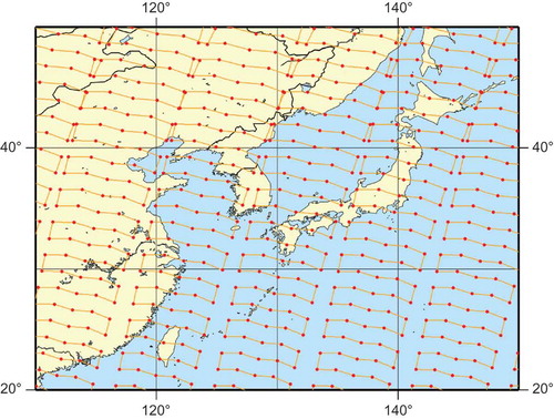
The orbit of GOSAT has a three-day recurrent period that includes 44 revolutions in three days. The distance between two adjacent orbits is about 900 km at the equator. To cover the whole globe, lattice point observations were made. At the beginning of satellite operation, a five-point observation mode in the cross-track direction was conducted. Figure 1 shows the nominal footprints of TANSO-FTS in the vicinity of Japan, in this case. Since August 2010, a three-point observation mode with three redundant observations at each location has been used. Over the ocean, sun-glint observations have been conducted because only sun-glint signals are strong enough in the SWIR spectral regions. This restriction has limited the latitudes of observations over the ocean. Details about GOSAT observations can be found in the literature (e.g. Kuze et al. 2012). Because GOSAT lattice observations provide sparse coverage over the globe, and because data observed only over cloud-free areas are processed into L2 retrieval, the regional distribution of retrieved GOSAT data is not uniform over the globe. In addition, the number of L2 data products (Ver. 02.**) of good quality released to general users is about 600–1000 per satellite recurrence (three days), primarily because of the influence of cloud and aerosol contaminants in the FTS field of view, and secondarily because of weak reflected signals due to low surface albedo and low solar zenith angles. This number of data points is insufficient to make a stable spatial interpolation globally.

Figure 1. Nominal footprints of TANSO-FTS in the vicinity of Japan.

To estimate the values of data in areas of the globe where no effective observations are made, we filled in the gaps by applying kriging to the L2 products and produced the TANSO-FTS SWIR Level 3 (L3) product. In L3 processing, XCO₂ and XCH₄ monthly mean values in each 2.5° latitude × 2.5° longitude mesh are statistically estimated from only L2 products.

There are several well-known methods for interpolating and extrapolating (referred to as ‘interpolation’ hereafter) two-dimensional surfaces; these include bilinear bi-cubic convolutions, the weighted average method, the minimum curvature method, and kriging. The kriging and minimum curvature methods have been the most commonly used interpolation methods in recent geostatistical applications (Cressie and Wikle 2011; Chiles and Delfiner 1999). Kriging was originally developed in the science of mining, but it is currently used in a wide variety of fields in the geophysical and geographical sciences (Chiles and Delfiner 1999; Qu et al. 2013). Kriging is a spatial statistical method for interpolating, or sometimes extrapolating, data. If suitable model parameters can be obtained by kriging, then this is considered better than the minimum curvature method because kriging takes a statistical approach to data analysis that reflects the statistics of the data over the whole globe. In addition, kriging gives estimates of interpolation errors which are referred to as minimum mean square errors (MMSE).

Hammerling, Michalak, and Kawa (2012) used GOSAT XCO₂ data produced by the Atmospheric CO₂ Observation from Space (ACOS) team (O’Dell et al. 2012). The ACOS XCO₂ data were retrieved from GOSAT radiance data within 2000 km of the target location. Hammerling, Michalak, and Kawa (2012) assumed that XCO₂ data were stationary within this area. This method is applicable to an L2 product with moderate spatial density, because the amount of data needed for the statistical calculation is compatible with the product. In contrast, Tomosada (2011) generated a semi-variogram using global data and conducted universal kriging to calculate XCO₂ at target points. To address the difficulties caused by assuming global stationariness and the problems caused by the large number of data in kriging, Tomosada (2011) used the Fixed Rank Kriging method proposed by Cressie and Johannesson (2008). On the one hand, Fixed Rank Kriging models a non-stationary field by a hidden, non-stationary process whose covariance or semi-variogram is assumed to be locally expressed by a fixed number of basis functions. In this paper, on the other hand, non-stationarity is not considered in the model and ordinary kriging is applied to the observational data within well-defined regions, whereas a semi-variogram is generated for the entire globe using global observational data. An example of the application of kriging to GOSAT data is the study by Liu et al. (2012), who discussed the application of the kriging method to GOSAT L2 data in East Asia and China under different circumstances.

In this paper, we first describe our kriging method and a semi-variogram model in Section 2. The method is then implemented by using it to analyse GOSAT L2 (XCO₂) data in Section 3. We evaluate our kriging method in Section 4.1, where we provide a comparison between the ‘ideal data’ and the ‘virtual data’ calculated from the ‘model data’, then in Section 4.2, where we make a comparison between ‘virtual data’ and ‘real data’. Finally we discuss the results of the comparison and the implications of the work in Section 5.

2. Method

In a kriging method, the spatial behaviour of the target parameter is characterized by the mode of continuous spatial random fields, and values of arbitrary points on the random field are estimated from observational data. There are several kinds of kriging, including, inter alia, simple kriging, ordinary kriging, co-kriging, and universal kriging (Wackernagel 2003). In this study, we adopted ordinary kriging based on the number of data to be used in the calculation, the simplicity of the calculation, and situations to be addressed in the following discussion.

In L2 products, XCO₂ and XCH₄ are stored, the distributions of which show characteristics of latitudinal dependence (e.g. differences in zonal means) and seasonal dependence (e.g. the NOAA GLOBALVIEW-CO2 2013 website). The characteristics of the distributed variables are therefore considered to be associated with random fluctuations superimposed on a distribution pattern. In this paper, the distribution of XCO₂ or XCH₄ is divided into two parts, latitudinal distribution and random fluctuations (see Equations (8) and (9)), and only the randomly fluctuating part is estimated by the ordinary kriging predictor. This randomly fluctuating field can be assumed to be uniform with a constant but unknown mean. In this situation, ordinary kriging is the best suited of the various kriging methods. Simple kriging is not applicable if the mean value of the field is unknown; co-kriging is a method used for multivariate fields and universal kriging is appropriate for fields with significant drift.

2.1. Kriging

In the ordinary kriging method, a predicted value at an arbitrary target point is estimated by considering the statistical properties of a set of observational data. This method predicts the observed value of an arbitrary point on this random field, the characteristics of which are a function of the statistical properties of the observational data. According to the formula of the kriging method, , the predicted value at an arbitrary point , is expressed as a weighted sum of the observational data:

(1)

where is the weighting factor at observation point , n is the total number of observation points to be used, and is the observed value at each point .

The methods of producing L3 products by ordinary kriging are described below.

2.1.1. Separating the distribution field

A distribution field F can be divided into a deterministic component m and a random field component .

The deterministic component m, which is called drift, is described by a function that expresses the pattern of spatial distribution. In this study, the drift was described by a linear function (see Equation (8)) that was estimated by applying a linear least-squares method to the L2 data. The drift m has a latitudinal pattern, because the XCO₂ or XCH₄ data have latitudinal distribution.

The random field was assumed to have a constant mean, and it was predicted by ordinary kriging.

The drift m and random field were defined for each month.

2.1.2. Ordinary kriging

Ordinary kriging is the best linear, unbiased predictor of an essentially stationary random field. The assumption is that the random variable on an arbitrary point has a constant but unknown mean.

It is assumed that a random variable has a finite second moment.

In ordinary kriging, the statistical component is expressed by semi-variograms. A semi-variogram is a function that describes the statistical characteristics of the spatial dependence of a random variable, and is defined as

(2)

for , = 1, 2, …, n. The term , which is the value of a random variable on an arbitrary point, is described by a linear combination of the known values (Equation (1)).

To predict a value of , the weight must be estimated. Ordinary kriging is a method of best linear prediction. The meaning of ‘best’ is that the mean squared error, , is minimized where is the true value at (Wackernagel 2003).

After applying the formula to the real data, this mean squared error is described with Equation (3) using the matrices and the vectors defined by Equation (4):

(3)

(4)

To minimize , a weighting vector can be calculated with Equation (5):

(5)

The MMSE, , is determined with Equation (6):

(6)

If all semi-variograms and are given, the weighting vector and the MMSE, , of arbitrary points on the random field can be estimated. To complete the calculation, a semi-variogram model must be calculated as described next.

2.2. Semi-variogram model

An empirical semi-variogram is used in kriging as the first estimate of the semi-variogram.

If the random field is an isotropic field, depends only on the distance h between the two locations.

From observational data , the empirical variogram is defined by the following equation:

(7)

where is the number of pairs of data locations such that (h generally means an approximate distance).

The empirical semi-variogram cannot be computed at any distance h, but ordinary kriging needs valid semi-variogram values at every distance. In applied ordinary kriging, the empirical semi-variograms are usually approximated by a model function. The semi-variogram models are restricted to avoid instability of the solution.

In a kriging application, some semi-variogram models are known as practical types. A typical semi-variogram model is shown in Figure 2, with definitions of technical terms.

Figure 2. Definitions of technical terms used in the method. The circles are semi-variograms and the solid curve is a semi-variogram model obtained by fitting a curve to the circles.

3. Implementation

The goals of this study were to estimate the statistically optimal distribution of the L2 data targeted for the GOSAT data over the globe and to make a reasonable global distribution map of greenhouse gases as an L3 product from only L2 data. To achieve these objectives, some preprocessing and post-processing were needed to apply our kriging method, and some suitable conditions had to be determined to apply the method. Figure 3 shows a flow chart for generating the L3 product.

Figure 3. Flowchart of the steps involved in creating FTS Level 3 products. The numbers in the boxes denote the section numbers in the manuscript.

3.1. Dividing the observed values into deterministic (latitudinal trend) and random variable components

The latitudinal pattern of L2 (XCO₂ or XCH₄) was estimated with a least-squares method using Equation (8). This latitudinal trend is also referred to as the deterministic component in the following sections. We assumed that the latitudinal pattern values of XCO₂ or XCH₄ could reasonably be approximated by a linear function of the sine of the latitude:

(8)

where is the latitude of location s, and a and b are constants to be determined by the latitudinal distribution of XCO₂ or XCH₄. The residual part , which is calculated by subtracting from the L2 value (Equation (9)), is assumed to be a random variable having the same mean, independent of the location. This variable can be used in the method of ordinary kriging:

(9)

3.2. Semi-variogram model function

In this study, we used the following exponential semi-variogram model by analogy to the actual distribution of the L2 data, because distribution of the L2 data empirically closely matched an exponential variogram model:

(10)

where is known as the nugget, as the sill, as the influence range, and h is the distance between two observation points (Figure 2). In some cases, an extremely large may be calculated. However, such cases, which are similar to a simple linear function, can still be considered to be a form of Equation (10). In this study, we therefore used the exponential variogram model for estimating , and we referred to ,, and as semi-variogram model parameters.

The earth was approximated in this study by a sphere with radius R, with the latitude and longitude information taken from the L2 product. The distance h between two locations, and , was calculated as the great circle distance using the following equation:

(11)

The radius of the earth was defined as

(12)

3.3. Estimating the semi-variogram model parameters over land and ocean

It is difficult to fill data-sparse areas to generate the semi-variogram model using local or regional semi-variogram models. For this reason, we selected a global semi-variogram model in this study. However, because there is a significant difference between semi-variograms for land and ocean (Figure 4), two different semi-variograms were therefore always generated in L3 processing. Because there are various kinds of sources (e.g. cities and factories) and sinks (e.g. forests) of greenhouse gases that are non-uniformly distributed over land, a semi-variogram curve over land tends to show relatively small values for small distances and to rapidly increase as distance increases. In contrast, a semi-variogram curve over the ocean is expected to have a relatively better correlation with long-range distribution of the gas. The two curves seem to be quite different, with that for land increasing rapidly near a distance of zero. The semi-variogram models for land and ocean were obtained from each of the empirical semi-variograms by fitting Equation (10) to the data with non-linear least-squares using the Levenberg–Marquardt algorithm. The empirical semi-variograms were made by averaging the variogram cloud within 100 km distance intervals. A practical algorithm requires some additional processing to avoid a gap between land and sea, a matter we do not address in this paper.

Figure 4. An example of empirical semi-variograms. Open circles and triangles denote semi-variograms obtained from data over ocean and land, respectively. Solid curves show empirical semi-variogram curves obtained by least-squares fitting of each semi-variogram plot.

3.4. Kriging calculation

After estimating the semi-variogram model using the entire global dataset, the values of all grid cells at a location were estimated using ordinary kriging. The locations of the cells were defined by 2.5° latitude × 2.5° longitude meshes for the following reason. Most GOSAT observations were made with five- or three-point modes in the cross-track direction of the satellite orbit. The distances between adjacent observation points were approximately 150 km and 250 km, respectively, for each mode at the equator. In the L3 product, the map projection is an equal-latitude/longitude projection (i.e. equi-rectangular projection). After considering these conditions (in the same order as the observational point distances at the equator mentioned above), we selected a grid size of 2.5° in latitude/longitude. This grid size corresponds to approximately 278 km in latitude and longitude at the equator. At the boundaries between land and ocean, the semi-variogram model for land was used when more than 50% of a grid cell was occupied by land; otherwise, the semi-variogram model for the ocean was used.

Because the semi-variogram has a negative exponential dependence on distance, as expressed in Equation (10), the influence of distant observations is much less than that of neighbouring ones. To reduce computational time, only observations that were influential within a predetermined distance were used for the kriging calculation. In fact, most of the semi-variograms approached constant values (sill), and over the range where the data values became very close to the sill, the correlation of the estimated value with the L2 data located outside of the range was very low. The algorithm in this study can be summarized as follows: although all observations over the globe were used for semi-variogram calculation, only those in the neighbourhood of the target points were used for the kriging calculation. This approach is called ‘regional kriging’ in this study. The magnitude of the range was fixed at 1000 km so that the kriging calculation was feasible with the number of data.

In regional kriging, a matrix defined by Equation (4) was generated for each grid cell using the L2 values from each observation. Each element of the matrix was generated using the values estimated with the semi-variogram for L2 data located in a specific range from the target grid cell. The same procedure was applied for the vector . Thus, the value of the target cell was calculated by using the method explained in Section 2. To make a reasonable calculation, the size of the matrix should be at least 10 × 10, that is, there should be more than 10 L2 data points in the area. When this condition was not satisfied, kriging was not applied to the cell.

3.5. Merging the trend and interpolated random variable

The random field component, which is the result of kriging, was merged in this step with the trend (deterministic component). When there were a sufficient number of L2 data in the ‘region’ neighbouring a grid cell located at a specific latitude and longitude, the field value was calculated by merging the trend and the random field:

(13)

In contrast, for each of the grid cells where a kriging calculation was not applied, only a trend value was applied:

(14)

In such a case, the estimated value was the same as the deterministic component at the mesh location.

Between the field values of cells with and without kriging, there were very large gaps in some cases. To smooth the difference, a Gaussian filter in 3 × 3 grid meshes was applied after the merger.

3.6. Masking

L3 data were generated covering all grids on earth but the uncertainty, which was evaluated with the ‘standard deviation map’ calculated from MMSE, depended on the values and/or distribution of the L2 data. It was preferable to remove estimated data with an extremely high MMSE. In this study, for any mesh for which there were no L2 data within a circle of radius of 500 km (determined experimentally), the data were masked in the L3 dataset.

4. Evaluations and applications

When confirming the results of our method, it was desirable to compare the interpolated L3 values to the ‘actual correct answers’. However, it is unrealistic to make this comparison because, in general, no actual data exist at the assumed locations. One of the best ways to check the performance is a cross-validation analysis; in this type of analysis, half of the L2 data are used to estimate an L3 map, and the agreement between this L3 map and the other half of the L2 data provides the check. Unfortunately, there were not enough L2 data to make this examination possible. Another potential way is to compare the L3 map to ‘virtual’ L2 data produced by a reliable atmospheric tracer transport model simulation. Hereafter, the CO₂ distribution simulated by such a method is termed the ideal L3 map. If the L3 map estimated by the kriging method is sufficiently similar to the ideal L3 map, it seems reasonable to conclude that the method is suitable from a practical standpoint. In the first part of this section, we show that the L3 map is in reasonable agreement with the ideal L3 map.

4.1. Evaluation of the method

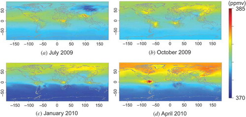
Virtual L2 maps were constructed using XCO₂ distributions calculated with the atmospheric tracer transport model (NIES transport model version 05, Maksyutov et al. 2008; Saeki et al. 2013). The NIES.05 model considers sources and sinks of CO₂ on the Earth’s surface. Some of these sources are associated with anthropogenic emissions. Emission inputs to the model include fluxes associated with fossil fuel burning, cement production, and biomass burning; terrestrial biosphere–atmosphere fluxes; and ocean–atmosphere fluxes. Representative maps of the global distribution of XCO₂ in the four seasons obtained with this model are shown in Figure 5. The model was able to produce global distribution averaged over one day with 1.0° × 1.0° resolution covering the whole globe. Each mesh of global distribution was further averaged in time over one month and in space over a 2.5° × 2.5° grid. The ideal L3 maps could then be compared to the GOSAT L3 products.

Figure 5. Global XCO₂ distributions simulated with the NIES.05 atmospheric tracer transport model. The average column density for one month is plotted in each panel. Each panel shows the monthly distribution in one of four representative months (seasons) in a year.

Figure 6 shows the virtual L2 distributions simulated with the model. Each value on the map was taken from the nearest grid in the ideal L3 maps at a location and time corresponding to each real L2 data point. The coloured dots correspond to the locations over which the satellite actually made observations and where L2 data were generated at least once during the month. Because the satellite traverses the same orbit about 10 times every month, there can be several data points from the same location in a month. Figure 7 shows semi-variograms plotted as a function of distance up to 4000 km during each month over both ocean and land. In general, the data plotted over ocean tend to oscillate, in some cases strongly, at a constant interval of distance. This interval reflects the orbital interval of the satellite over ocean, as shown in Figure 6.

Figure 6. Virtual XCO₂ distributions simulated with the NIES.05 atmospheric tracer transport model.

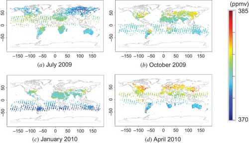
Figure 7. Semi-variograms and semi-variogram curves estimated from the virtual L2 data shown in Figure 6. Each open circle and triangle was obtained from data over ocean and land, respectively. Solid curves show semi-variogram models obtained by least-squares fitting of each semi-variogram. The values calculated by the models are used to construct semi-variogram matrices. Each panel corresponds to the analogous panel in Figure 5.

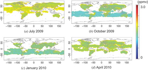
The resulting L3 maps and their standard deviation maps (see Equation (6)) are shown in Figures 8 and 9, respectively. We have used the term ‘standard deviation’ to mean the square root of the MMSE. The panels in Figure 8 are subsets (without masked areas) of the results of model simulation of the corresponding panels in Figure 5. The standard deviations show that the estimations can be done with relatively small errors of less than about 0.5 ppm. In Figure 9, especially in panel (d), a striped pattern is apparent over the ocean. This striping corresponds to the orbital distance of the satellite: the errors are smaller in densely observed regions and larger in sparsely observed regions. The differences between the ideal L3 data and the estimated L3 maps calculated from virtual L2 data are plotted in Figure 10, where the latter data are subtracted from the former. Histograms of the differences, shown in Figure 11, indicate that the differences were centred at approximately zero, with standard deviations less than 0.5 ppmv in every case, and that the absolute values of the difference were at most 3 ppmv. Most of the differences were smaller than 2 ppmv, which is almost comparable to the magnitude of differences between the XCO₂ data and validation results (Yoshida et al. 2013). This result shows that reasonable estimations can be made by using the kriging method. In general, however, real L2 data include both observational errors and data-retrieval errors and we do not expect the real L2 data to have the same quality as virtual L2 data. The errors in real data can be larger than those in virtual data.

Figure 8. L3 maps calculated from the virtual L2 maps shown in Figure 6. Each panel corresponds to the analogous panel in Figure 5.

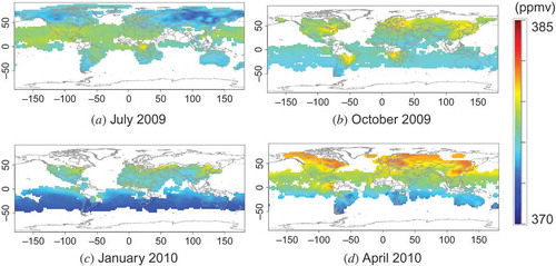
Figure 9. Standard deviation maps for the L3 maps shown in Figure 6. Each panel corresponds to the analogous panel in Figure 5.

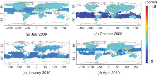
Figure 10. Difference between the ‘ideal’ XCO₂ distribution shown in Figure 5 and the reconstructed XCO₂ distribution obtained by kriging (Figure 8). The white zones are areas where values cannot be determined by the method used there. Each panel corresponds to the analogous panel in Figure 5.

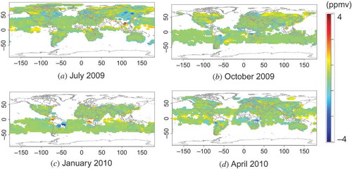
Figure 11. Histograms of the data plotted in Figure 10. Each graph corresponds to the analogous panel in Figure 5.

4.2. Application to GOSAT data

This section shows some examples of L3 maps obtained by applying our method to real L2 data. The L2 maps of XCO₂ retrieved from FTS Level 1 B products are shown in Figure 12. Every coordinate of the observation points in these maps is the same as the corresponding coordinate of the virtual L2 maps in Figure 6. Figure 13 shows corresponding semi-variograms plotted as a function of distance up to 4000 km in each month over both ocean and land. The resulting L3 maps and corresponding ‘standard deviation’ maps are shown in Figures 14 and 15, respectively.

Figure 12. Real L2 maps retrieved from GOSAT Level 1 B products.

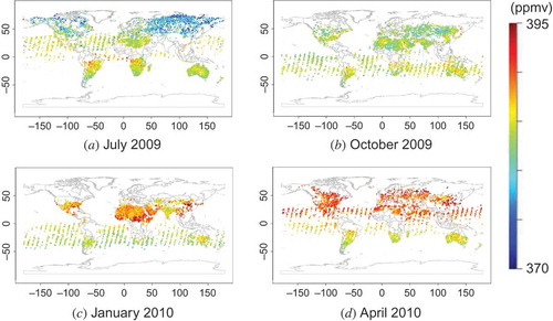
Figure 13. Semi-variograms and semi-variogram curves estimated from the real L2 maps shown in Figure 12.

Figure 14. Real L3 maps estimated from the real L2 maps shown in Figure 12.

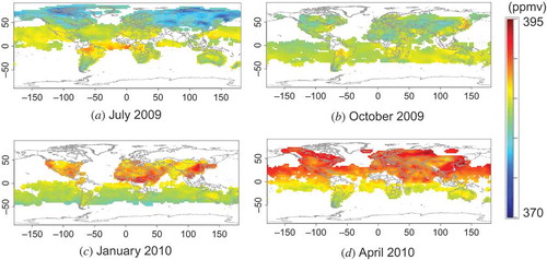
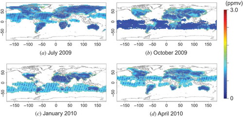
Figure 15. Standard deviation maps for the L3 maps shown in Figure 14.

It is initially apparent that the L3 products (Figure 14) are similar to the L2 maps (Figure 12), although the former cover more area globally than the latter. However, a comparison of the virtual semi-variograms calculated from the virtual model data (Figure 7) to the semi-variograms calculated from the observed data (Figure 13) reveals that, although the general trends of the semi-variograms are similar, the values of the semi-variograms are higher for the real data. The corresponding L3 products (see Figures 9 and 15) show that the standard deviations over land are about 0.5 and 1.5 ppmv for the virtual and real observations, respectively. We discuss these differences in Section 5.2.

5. Discussion and Conclusions

5.1. Discussion

The major objective of this study was to show that the proposed statistical algorithm for generating a GOSAT L3 product by using only GOSAT L2 products provides a reasonable overview of the global distribution of monthly XCO₂ and XCH₄ over both land and ocean in regions near the observational L2 data.

With respect to temporal resolution, the L3 product was generated every month. Even when there were very high or very low values of XCO₂ or XCH₄, those data would have been averaged and merged in the mesh of the monthly map. They are therefore not detectable in the L3 maps. However, seasonal changes in XCO₂ and XCH₄ are discernible in the L3 products (Figure 14).

With respect to spatial resolution, the L3 product was generated for meshes with dimensions of 2.5° in both latitude and longitude. This grid size seems reasonable when consideration is given to the GOSAT lattice observation distances and the present rate at which FTS SWIR L2 data are retrieved. However, as discussed in Section 1, etc., there are large areas that lack L2 data at this spatial resolution, especially over the high-latitude areas of the ocean and areas contaminated with clouds and aerosols. We masked these areal gaps to avoid misunderstanding. The extent of this problem is dependent on the number of remaining SWIR observations, that is, on the trade-off between data quality and amount of data. The current L3 product is based on the same limited number of GOSAT L2 SWIR products released to the general public.

The GOSAT Level 4 B (L4 B) product, which covers the whole globe by adding external data to the L2 data, is, in terms of use of scientific data, more reliable than the L3 product for providing global maps. However, the model needs several kinds of carbon flux databases, including anthropogenic emissions, biomass burning data, terrestrial biosphere–atmosphere fluxes, and ocean–atmosphere fluxes. Also needed are ground-based observational CO₂ data, which take about 1 year after the measurements to be made available officially to users, in addition to satellite L2 data. Moreover, the estimation of carbon sources and sinks from inverse modelling by use of an atmospheric tracer transport model should be a batch process that uses data from several previous months. It would therefore take about 1 year to publish L4 B data after satellite measurements. In addition to the issue of processing speed, these results would require large computational resources. In contrast, L3 maps produced using the kriging method use smaller computational resources and require the accumulation of just one month of L2 data. The processing speed and small computational burden of L3 maps are their major advantages for providing an overview of the global distribution of greenhouse gases in time and space. Because of these advantages, the L3 product can play an important role by providing maps of monthly global distribution to users within only a few months of observations.

There are several ways to produce L3 maps, each with its own characteristics. We have shown that the proposed method works reasonably well for the case of satellite-derived greenhouse gas data, such as GOSAT L2 products. We also compared our method, which uses a global semi-variogram and applies local kriging, to another typical kriging method (Hammerling, Michalak, and Kawa 2012) that estimates local semi-variograms and applies local kriging. Because the data used are not the same, direct comparison to the results of this method is difficult. The general trends of these results, however, do not seem to be significantly different to the extent that the corresponding L2 data are similar. This result shows that either our method or theirs is applicable to the actual GOSAT L2 data, depending on the amount of available data. GOSAT FTS SWIR L3 products, which have been processed with the kriging method presented here, will be available to the general public from the GOSAT data distribution website (https://data.gosat.nies.go.jp/).

5.2. Concluding remarks

In this study, we developed an interpolation algorithm to generate the FTS SWIR L3 product (monthly averaged global XCO₂ or XCH₄). The algorithm uses only FTS SWIR L2 products as input data for every month.

We used an ordinary kriging method as the interpolation method. Because the mean global distribution of greenhouse gases is associated with a significant latitudinal pattern, this pattern was approximated by a linear function of the sine of the latitude and separated from the original data. The residuals were treated as random variables to be interpolated by kriging.

Because it was intended that this product would cover the whole globe as much as possible, only two semi-variograms were generated globally, one each for land and ocean. The design of these two semi-variograms took into consideration the differences of the source/sink mechanisms and observation patterns over land and ocean.

Using the data simulated from the NIES.05 atmospheric tracer transport model, we made a quantitative evaluation of this algorithm. On the one hand, the results showed that the means of the differences between the ideal maps and the virtual L3 maps were approximately zero, with a standard deviation less than 0.5 ppmv in every case. On the other hand, a comparison was made between Figure 9 (standard deviation from the virtual model) and Figure 15 (standard deviation from the real data). As mentioned in Section 4.2, it is apparent that the latter is larger than in the former in magnitude, specifically by about 1.5 ppmv over land. Nevertheless, we should remember that the MMSE of the kriging prediction given by Equation (6) is the sum of the squared estimation error () and the squared observation error (). We should therefore not compare Figure 9 directly to Figure 15, because both should be versions of the estimation errors, free of observation errors. The square of the estimation error τ is calculated by subtracting a new error corresponding to the nugget θ₁ = σ_ε² (see Equation (10)) from the MMSE:

(15)

The estimation error for the real data is shown in Figure 16. As is apparent from Figure 16, is in the order of 0.5 ppmv, equivalent to the standard deviation error of the virtual model (Figure 9).

Figure 16. Estimation error, , for the real data.

GOSAT completed five years of nominal operation on 23 January 2014 and is now in its extended operation period. The pointing mechanism of GOSAT is slightly unstable, but it is still working without serious problems. We expect that GOSAT will operate for several more years, and the GOSAT Project will produce and distribute useful data products to registered researchers and general users for the time being. The FTS SWIR Level 3 data product, which is generated by the kriging method proposed here, will be available to users following publication of this paper.

Disclosure statement

No potential conflict of interest is reported by the authors.

Acknowledgements

We thank the members of JAXA, the Ministry of the Environment, and NIES for their roles in the GOSAT Project. We also thank Dr M. Tomosada of the Central Research Institute of the Electric Power Industry (Japan), Dr A.M. Michalak of the Carnegie Institution for Science, and Dr D. Hammerling of the Statistical and Applied Mathematical Sciences Institute for their helpful discussions. The GPV (Grid Point Value) data of the Japan Meteorological Agency were used as reference data in the GOSAT TANSO-FTS L2 retrievals.

References

- Chiles, J.-P., and P. Delfiner. 1999. Geostatistics, Modeling Spatial Uncertainty, Wiley Series in Probability and Statistics. Hoboken, NJ: John Wiley & Sons.
- Cressie, N., and G. Johannesson. 2008. “Fixed Rank Kriging for Very Large Spatial Data Sets.” Journal of the Royal Statistical Society: Series B (Statistical Methodology) 70: 209–226. doi:10.1111/j.1467-9868.2007.00633.x.
- Cressie, N., and C. K. Wikle. 2011. Statistics for Spatio-Temporal Data. Hoboken, NJ: Wiley.
- Hammerling, D. M., A. M. Michalak, and S. R. Kawa. 2012. “Mapping of CO2 at High Spatiotemporal Resolution Using Satellite Observations: Global Distributions from OCO-2.” Journal of Geophysical Research 117: D06306. doi:10.1029/2011JD017015.
- Kuze, A., H. Suto, M. Nakajima, and T. Hamazaki. 2009. “Thermal and Near Infrared Sensor for Carbon Observation Fourier-Transform Spectrometer on the Greenhouse Gases Observing Satellite for Greenhouse Gases Monitoring.” Applied Optics 48: 6716–6733. doi:10.1364/AO.48.006716.
- Kuze, A., H. Suto, K. Shiomi, T. Urabe, M. Nakajima, J. Yoshida, T. Kawashima, Y. Yamamoto, F. Kataoka, and H. Buijs. 2012. “Level 1 Algorithms for TANSO on GOSAT: Processing and On-orbit Calibrations.” Atmospheric Measurement Techniques 5: 2447–2467.doi: 10.5194/amt-5-2447-2012.
- Liu, Y., X. Wang, M. Guo, and H. Tani. 2012. “Mapping the FTS SWIR L2 Product of XCO2 and XCH4 Data from the GOSAT by the Kriging Method – a Case Study in East Asia.” International Journal of Remote Sensing 33 (10): 3004–3025. doi:10.1080/01431161.2011.624132.
- Maksyutov, S., P. K. Patra, R. Onishi, T. Saeki, and T. Nakazawa. 2008. “NIES/FRCGC Global Atmospheric Tracer Transport Model: Description, Validation, and Surface Sources and Sinks Inversion.” Journal of the Earth Simulator 9: 3–18.
- National Oceanic and Atmospheric Administration (NOAA) Earth System Research Laboratory. 2013. “GLOBALVIEW-CO2: Documentation.” NOAA Earth System Research Laboratory. http://www.esrl.noaa.gov/gmd/ccgg/globalview/co2/co2_documentation.html
- O’Dell, C. W., B. Connor, H. Bösch, D. O’Brien, C. Frankenberg, R. Castano, M. Christi, D. Eldering, B. Fisher, M. Gunson, J. McDuffie, C. E. Miller, V. Natraj, F. Oyafuso, I. Polonsky, M. Smyth, T. Taylor, G. C. Toon, P. O. Wennberg, and D. Wunch. 2012. “The ACOS CO2 Retrieval Algorithm – Part 1: Description and Validation Against Synthetic Observations.” Atmospheric Measurement Techniques 5: 99–121. doi:10.5194/amt-5-99-2012.
- Qu, Y., C. Zhang, D. Wang, P. Tian, W. Bai, X. Zhang, P. Zhang, H. Dai, and Q. Wu. 2013. “Comparison of Atmospheric CO2 Observed by GOSAT and Two Ground Stations in China.” International Journal of Remote Sensing 34 (11): 3938–3946. doi:10.1080/01431161.2013.768362.
- Saeki, T., R. Saito, D. Belikov, and S. Maksyutov. 2013. “Global High-Resolution Simulations of CO2 and CH4 Using a NIES Transport Model to Produce A Priori Concentrations for Use in Satellite Data Retrievals.” Geoscientific Model Development 6: 81–100. doi:10.5194/gmd-6-81-2013.
- Tomosada, M. 2011. “A Prediction Method for the Global Distribution of CO2 Concentration from Irregularly Observed Locations.” Procedia Environmental Sciences 7: 134–139. doi:10.1016/j.proenv.2011.07.024.
- Wackernagel, H. 2003. Multivariate Geostatistics. Berlin: Springer.
- Yoshida, Y., N. Kikuchi, I. Morino, O. Uchino, S. Oshchepkov, A. Bril, T. Saeki, N. Schutgens, G. C. Toon, D. Wunch, C. M. Roehl, P. O. Wennberg, D. W. T. Griffith, N. M. Deutscher, T. Warneke, J. Notholt, J. Robinson, V. Sherlock, B. Connor, M. Rettinger, R. Sussmann, P. Ahonen, P. Heikkinen, E. Kyrö, J. Mendonca, K. Strong, F. Hase, S. Dohe, and T. Yokota. et al. 2013. “Improvement of the Retrieval Algorithm for GOSAT SWIR XCO2 and XCH4 and Their Validation Using TCCON Data.” Atmospheric Measurement Techniques 6: 1533–1547. doi:10.5194/amt-6-1533-2013.