A new method to generate a high-resolution global distribution map of lake chlorophyll

Abstract

A new method was developed, evaluated, and applied to generate a global dataset of growing-season chlorophyll-a (chl) concentrations in 2011 for freshwater lakes. Chl observations from freshwater lakes are valuable for estimating lake productivity as well as assessing the role that these lakes play in carbon budgets. The standard 4 km NASA OceanColor L3 chlorophyll concentration products generated from MODIS and MERIS sensor data are not sufficiently representative of global chl values because these can only resolve larger lakes, which generally have lower chl concentrations than lakes of smaller surface area. Our new methodology utilizes the 300 m-resolution MERIS full-resolution full-swath (FRS) global dataset as input and does not rely on the land mask used to generate standard NASA products, which masks many lakes that are otherwise resolvable in MERIS imagery. The new method produced chl concentration values for 78,938 and 1,074 lakes in the northern and southern hemispheres, respectively. The mean chl for lakes visible in the MERIS composite was 19.2 ± 19.2, the median was 13.3, and the interquartile range was 3.90–28.6 mg m⁻³. The accuracy of the MERIS-derived values was assessed by comparison with temporally near-coincident and globally distributed in situ measurements from the literature (n = 185, RMSE = 9.39, R² = 0.72). This represents the first global-scale dataset of satellite-derived chl estimates for medium to large lakes.

1. Introduction

Freshwater lakes are integral in the provisioning of ecosystem services and maintenance of biodiversity (Wilson and Carpenter 1999; Dudgeon et al. 2006). Though lakes, ponds, and impoundments only represent in the order of 3–4% of the global non-glaciated land surface (Verpoorter et al. 2014; Downing et al. 2006), they are frequently highly productive, with disproportionately large net C fluxes compared with terrestrial systems (Cole et al. 2007). Lakes also provide habitat for freshwater fish – an important food source in many areas of the world (Welcomme 2011) – as well as other organisms representing an estimated 6% of all described species (Dudgeon et al. 2006). Many freshwater lakes are currently undergoing rapid change due to climate shifts, anthropogenic perturbations, and introductions of non-native species (e.g. Ficke, Myrick, and Hansen 2007; Adrian et al. 2009; Revenga et al. 2005; Vitousek et al. 1997; Strayer 2010). Many of these lake changes can be directly or indirectly characterized by changes in colour-producing agents (CPAs) (i.e. the bio-geochemical constituents of the water column that affect the water’s spectra, the primary CPAs being chlorophyll, suspended minerals, and coloured dissolved organic matter (Shuchman et al. 2013)). Chlorophyll is of particular potential value as a proxy for trophic state, primary production, and total ecosystem productivity (Lyche-Solheim et al. 2013). Thus, the capacity to monitor the water properties of freshwater lakes at a global scale via ocean colour satellites on an annual and intra-annual basis would provide important information to researchers, resource managers, and environmental regulators.

Relative to the open ocean (case 1 waters), where water colour is strongly dominated by the concentration of phytoplankton (Yentsch 1960), it is much more difficult to accurately estimate chlorophyll concentrations from multispectral imagery for coastal and inland (case 2) waters, where water colour is influenced by multiple CPAs that exhibit independent and considerable variations (Doerffer, Sorensen, and Aiken 1999; Morel and Prieur 1977). Added to this, many freshwater lakes are at least partly optically shallow, meaning that the water is shallow enough that the contribution of radiance reflected by the lake bottom to the light detected by ocean colour sensors is potentially significant. Numerous techniques for remote sensing of water quality parameters in inland waters have recently been proposed, and which are newly reviewed by Palmer, Kutser, and Hunter (2015). In brief, these inland techniques can be roughly categorized into two groups. The first group, semi-analytical bio-optical inversion models, were developed for the coastal ocean (Lee, Carder, and Arnone 2002; Maritorena, Siegel, and Peterson 2002) and inland waters (Shuchman et al. 2013; Korosov et al. 2009) and frequently rely on hyperspectral imagery and require tuning to local/regional inherent optical properties (IOPs) for accuracy, making them difficult to scale up to the global level (Sathyendranath 2000; Lee 2006). The second group is comprised of empirical approaches, including band ratio algorithms (O’Reilly et al. 1998, 2000; Gons, Rijkeboer, and Ruddick 2002; Binding, Greenberg, and Bukata 2012), which statistically relate the remotely sensed signal directly to chl (see review by Matthews 2011). Due to the optical complexity of inland waters described above, many researchers have presumed that an empirical approach general enough for application at the global level would not be sufficiently accurate to provide useful information on inland waters (Bukata 2005).

Various empirical ocean colour chlorophyll algorithms using satellite data from the CZCS, SeaWiFS, MODIS, MERIS and VIIRS sensors have been used successfully to estimate chl concentrations for single large lakes (100 km² or larger) or small groups of large lakes throughout the globe (Chavula et al. 2009; Wu et al. 2009; Odermatt et al. 2008; Vos et al. 2003; Lesht, Barbiero, and Warren 2012). The chl estimates for these lakes are relatively robust, though frequently overestimating low chl concentrations and underestimating high ones (Stramska et al. 2003; Cota, Wang, and Comiso 2004). The accuracy of these estimates is due in large part to the many pixels available for lake-wide averaging and the fact that large lakes have more ocean-like open pelagic zones and are therefore less dominated by terrestrial inputs of suspended materials other than phytoplankton that can have significant optical effects (Lesht, Barbiero, and Warren 2012; Matthews 2011). The successful use of empirical ocean colour satellite data to estimate chl in smaller lakes (between 0.5 and 100 km²) is far less documented (but see Koponen et al. 2004; De Moraes Novo et al. 2006) and until now simulated data have been used more frequently (e.g. Gitelson et al. 2009; Simis et al. 2007; Kallio et al. 2001).

The freshwater lakes of the world vary greatly in size, with the frequency of lakes increasing sharply with decreasing surface area (Verpoorter et al. 2014; Downing et al. 2006). The Global Lakes and Wetlands Database assembled by the World Wildlife Fund includes approximately 170,000 lakes with surface area >1 km² (Lehner and Döll 2004), and recent estimates have increased this estimate to approximately 200,000 (Downing et al. 2006) or 350,000 (GLOWABO database, Verpoorter et al. 2014). These high numbers are in sharp contrast to the fewer than 20 lakes worldwide larger than 10,000 km². Of currently available technologies, only empirical ocean colour satellite estimations make the monitoring of medium-sized and larger freshwater lakes feasible at a global scale. Even considering that most lakes smaller than 1 km² are not resolvable by any existing ocean colour satellite, monitoring the hundreds of thousands of lakes >1 km² poses a significant technical challenge.

We proposed that empirical ocean colour satellite data can be used to generate estimates of the global distribution of chlorophyll concentrations in inland lakes with an accuracy sufficient to be useful for examining spatial patterns and temporal changes. To address this hypothesis, the utility and limitations of different ocean colour satellite products were evaluated and a method was developed to derive chlorophyll estimates from MERIS data for as many lakes throughout the world as possible. This new method was validated by comparison to in situ chlorophyll measurements compiled from the literature and representing a wide range of lake sizes and locations. The method was then applied to generate a 1 km-resolution global estimate of chlorophyll concentrations for lakes in both the northern and southern hemispheres during their respective growing seasons for the year 2011. We present a discussion of why standard NASA products are not sufficiently representative of global freshwater lakes for rigorous modelling activities, followed by a narrative of the development of an improved product. A comparison of the distribution of chl values from this more representative snapshot to those obtained from the standard OC4 MERIS chl product is provided. Additionally, we highlight some of the patterns observed in the global growing-season chlorophyll snapshot for the year 2011.

2. Methods

2.1. Global-scale estimation of inland lake chl concentrations

In this section, we describe the need for a custom method to generate a global satellite chl product for inland lakes. First we summarize the limitations of available standard global products, followed by the rationale for selecting MERIS as the data source and a description of the method developed by Michigan Tech Research Institute (MTRI) to produce the global snapshot product.

2.1.1. Limitations of NASA standard products

We began by reviewing the chlorophyll-a data products derived from MODIS Aqua and MERIS using the respective OC3 and OC4 blue–green band ratio algorithms, available as standard products from the NASA OceanColor data facility operated by the Ocean Biology Processing Group (OBPG, http://oceancolor.gsfc.nasa.gov). Although a number of methods could be used to estimate lake chlorophyll at the global scale, the NASA OC algorithms are among the best-known and thoroughly validated for estimating chlorophyll. The latest available data versions for each sensor were used (see http://oceancolor.gsfc.nasa.gov/WIKI/OCReproc.html for details). The multi-mission reprocessing described in detail at the referenced link has led to high consistency between the chl products from these different sensors. NASA has found that standard MERIS estimates tend to be lower than MODIS in eutrophic waters (chl concentration between 1 and 10 mg m⁻³), but without a robust in situ dataset, it is unclear which is more correct (Franz 2013).

Landsat imagery was not considered as an alternative to ocean colour sensors, despite the advantage of 30 m pixel resolution, for several reasons including the lack of a robust globally applicable chlorophyll retrieval algorithm (non-optimum spectral bands for chlorophyll retrieval), the absence of an efficient atmospheric correction approach, and the much less frequent satellite revisit time (16 days vs. ~daily for ocean colour platforms). Apart from these issues, a global Landsat dataset would pose a significantly higher computational burden.

We first evaluated the 4 km Level-3 reduced-resolution standard mapped image (SMI) MODIS OC3 and MERIS OC4 products, which are available as global layers composited over a range of time intervals, to determine how much information about global freshwater lakes could be obtained as a ready-to-use product. As expected, we found that the 4 km pixels limited the number of inland lakes for which chl could be estimated and the amount of information that could be extracted for those lakes. The 4 km version of the entire mission composite for each sensor, representing the maximum number of lakes resolvable with these data products, contained pixels with valid chl values for only 866 lakes for MODIS and 923 lakes for MERIS. Thus, a method for producing a finer-scale global freshwater product from a lower OC product level was necessary.

2.1.2. Sensor selection

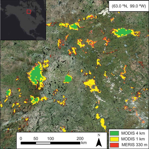
Initially, we planned to custom composite the daily Level-2 MODIS OC3 chlorophyll product (1 km resolution) into a global-scale 1 km map. Late in fall 2013, however, the 300 m MERIS full-resolution full-swath (FRS) global dataset became available for use through the NASA-ESA data sharing collaboration. We compared the utility of this newly available dataset to the Level-2 MODIS product for a sample area in the Canadian Shield in terms of the amount of surface water for which chl values were retrieved. We found that MERIS imagery retrieved approximately 9% more water surface area than MODIS due to MERIS’s smaller pixel size. In Figure 1, the green areas indicate the 4 km pixels retrieved by the MODIS L3 product, the yellow areas represent the gains in the mapped area made by using a 1 km custom composite rather than the L3 product, and the red areas indicate the further increase in retrievals achieved by utilizing MERIS rather than MODIS.

Figure 1. Example of the area of surface water retrieved by the MODIS L3 4 km product (represented in green) and the additional areas gained by using the MODIS 1 km composite (in yellow) and MERIS FRS imagery (in red) for an area in the Canadian Shield (centre of image 63.0° N, 99.0° W). MERIS retrieves the most information (green + yellow + red areas). The inset map at top left indicates the location of the example area.

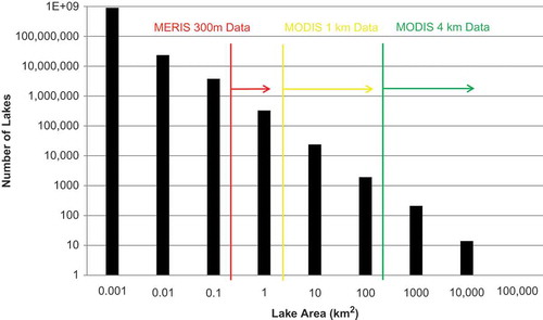
Based on this increase in mappable lake area, it was decided to utilize MERIS as the ‘workhorse’ ocean colour sensor for this global analysis because of the high perceived importance of minimum resolvable lake size and despite the fact that MERIS ceased to operate in early 2012. Figure 2 illustrates the relationship between lake surface area, the approximate global number of lakes in each size range as estimated by Verpoorter et al. (2014), and satellite spatial resolution. These thresholds do not account for shoreline complexity, which made many lakes non-retrievable with MERIS despite a surface area much larger than a MERIS pixel. Based on the relationship between lake size and satellite resolution shown in Figure 2, the MODIS 4 km product would be expected to retrieve chl values for approximately 1000 lakes worldwide, which is similar to the value of 866 that we obtained in practice. The use of 1 km MODIS imagery provides information on a substantially larger estimated number of lakes, approximately 19,000 worldwide based on the Figure 2 relationship. The even finer-resolution MERIS data have the potential to map chl distribution for lakes ≥ ~1 km², numbering approximately 170,000 in the Global Lakes and Wetlands Database (GLWD) shapefile, though as noted, a substantial fraction of those were determined to be non-retrievable due to their complex shorelines (high shoreline development ratio). The findings reported here for MERIS will be highly relevant to the inland chl retrieval abilities of OLCI, a new ocean colour sensor based on the design of MERIS, which is part of the instrument package planned for the Sentinel-3 mission and with the first satellite scheduled for launch in 2015.

Figure 2. Log-log plot of lake size vs. global lake frequency, annotated with the minimum resolvable lake sizes for MODIS 4 km and 1 km composites and MERIS 300 m data. Column values derived from Verpoorter, Kutser, and Tranvik 2014.

2.1.3. MTRI method and generation of global chlorophyll snapshot

Figure 3 is a flow chart summarizing the steps of the MTRI method for generation of a global chlorophyll snapshot for the northern and southern hemispheres, respectively, from MERIS OC4 data. These steps were necessary to retrieve the lakes that are not included in the L3 product due to both its coarser spatial resolution and issues with the NASA ocean discipline processing system (ODPS) land/water mask (a global layer used to mask out non-water pixels in the production of all NASA Level 2 standard OC products). Reviewing examples of the standard Level 2 MERIS OC4 product, it was noted that chl estimates were not obtained for a surprising number of lakes for which we would expect chl to be retrievable by MERIS based on their shape and area. We determined that the land/water mask was masking out many otherwise valid inland chl pixel values. To retrieve these masked lakes, it was necessary to download the Level 1A versions of MERIS imagery for August and February 2011 for the northern and southern hemispheres and process the L1A files to L2 using the SeaWiFS data analysis system software (SeaDAS, version 7.0) without using the ODPS land/water mask. August and February were selected to represent the growing season for the northern and southern hemispheres, respectively, based on a preliminary analysis indicating that use of these months would yield the largest number of ice-free lakes and provide values representative of the vegetation growing season. In addition to not utilizing the standard land/water mask, we used ocean processing for all image pixels (both land and water). The L2 data processed in-house were then averaged for a global 330 m grid, dividing the globe into 30° tiles to alleviate the computational burden. Chl retrieval values less than 0.15 or greater than 100 mg m⁻³ were masked, as concentrations beyond these thresholds are outside the range of values for which MERIS OC4 produces reliable estimates (Hu, Lee, and Franz 2012; NASA 2010). Finally, as shown in Figure 3, the cells of the global grid were analysed using the GLWD database as the source of geographic information on lake shorelines to calculate mean chlorophyll values for retrievable lakes.

Figure 3. Steps involved in the MTRI method for processing MERIS OC4 chl data at the global scale.

Given the volumes of data involved in compositing daily MERIS images into a global product, a Wget-based tool (Niksic 1998) was developed to quickly download large amounts of OceanColor data via FTP for specified areas and date ranges. This was used to obtain imagery both for specific lakes and times to support the validation analysis, and for all lakes during the selected summer 2011 months to produce chl estimates for a high number of lakes in a single recent year.

The Level 2 MERIS OC4 data processed in-house from L1A were composited for August 2011 for the northern hemisphere and for February 2011 for the southern hemisphere to create a ‘global summer’ product representing growing-season chl estimates for both hemispheres.

2.2. Validation with in situ data and ancillary environmental information

2.2.1. Global in situ chl dataset

In situ chlorophyll-a data were obtained by literature review (searching online databases using Google Scholar and ISI Web of Science), through direct contact with environmental agencies in North America, and from online databases (e.g. US Environmental Protection Agency’s STORET water quality data repository; http://www.epa.gov/storet/). For inclusion in the validation dataset, in situ lake chl data were required to represent a lake sufficiently large for MODIS and/or MERIS to obtain pixels uncontaminated by shoreline reflectance, to correspond to dates when MERIS was operational (2002–2012), and to represent a date or date range spanning five months or less. The threshold of five months was selected because values averaged over longer time spans included too much seasonal variation for a useful comparison. Additionally, many reports provide in situ chl values for a calendar year without including information on the actual sampling dates used to generate those values, and such data are likely not comparable to a satellite composite of all cloud- and ice-free dates in that year. When in situ measurements were reported for multiple locations within a lake for a known time frame, the average was taken to represent the whole lake. The lakes included in the validation dataset and the sources of the in situ chl data are summarized in Table 1.

Table 1. Sources of in situ chlorophyll-a data for the 37 lakes included in the in situ/satellite comparison.

	Lake	Latitude (°)	Longitude (°)	Source of in situ data
1	Cass Lake	47.4226	−94.5476	US EPA STORET, http://www.epa.gov/storet/dbtop.html
2	Upper Red Lake	48.1308	−94.9147	US EPA STORET
3	Pelican Lake	48.0620	−92.9055	US EPA STORET
4	Center Hill Reservoir	36.0053	−85.7420	US EPA STORET
5	Barkley Reservoir	36.8070	−87.9585	US EPA STORET
6	Old Hickory Reservoir	36.3092	−86.1897	US EPA STORET
7	J. Percy Priest Reservoir	36.0853	−86.5517	US EPA STORET
8	Angostura Reservoir	43.3048	−103.4469	US EPA STORET
9	Lake Sinai	44.2660	−97.0780	US EPA STORET
10	Lake Poinsett	44.5650	−97.0802	US EPA STORET
11	Lake Kampeska	44.9256	−97.2102	US EPA STORET
12	Waubay Lake	45.4247	−97.4004	US EPA STORET
13	Sharpe Lake	44.1688	−99.7316	US EPA STORET
14	Bitter Lake	45.2804	−97.3084	US EPA STORET
15	Lake Francis Case	43.1463	−98.7786	US EPA STORET
16	Lake Michigan	44.0135	−86.7611	US EPA STORET
17	Lake Saint Clair	42.4571	−82.6774	US EPA STORET
18	Kootenay Lake	49.5953	−116.8172	Schindler et al. (2006)
19	Lake Taihu	31.2003	120.1909	Zhang, Qin, and Liu (2007)
20	Ramsagar Reservoir	25.6685	78.3960	Khondker et al. (2012)
21	Lake Malawi	−11.9884	34.5110	Van Der Sande et al. (2012)
22	Lake of the Woods	49.2410	−94.6675	Pla et al. (2005)
23	Lake Champlain	44.6126	−73.3065	US EPA STORET
24	Lake Ladoga	60.8311	31.4758	Viljanen et al. (2008)
25	Lake Baikal	53.3998	107.6614	Heim et al. (2005)
26	Volgogradskoe Reservoir	50.4187	45.6643	Nemirovskaya (2012)
27	Lake Calamus	41.8681	−99.2568	US EPA STORET
28	Lake Tana	12.0117	37.3142	Wondie et al. (2007)
29	Amisk Lake	54.5674	−102.2345	ALMS (2008)
30	Lake Chaohu	31.5679	117.5312	Yang et al. (2013)
31	Toba Lake	2.6069	98.8107	Barus, Sinaga, and Tarigan (2008)
32	Ir H Juanda (Djuanda) Reservoir	−6.5501	107.3367	Garno (2003)
33	Tonle Sap Lake	12.8849	104.0722	Campbell et al. (2006)
34	Lake Apopka	28.6237	−81.6261	US EPA STORET
35	Lake Harris	28.7775	−81.8154	US EPA STORET
36	Funil Reservoir	−22.5525	−44.6073	Soares et al. (2009)
37	Laguna de Rocha	−34.6188	−54.2895	Piccini et al. (2006)

2.2.2. Global lakes and wetlands database

This study also made use of the most comprehensive available global-scale GIS database of lake and reservoir boundaries, the GLWD (Lehner and Döll 2004). The GLWD represents a compilation of numerous existing maps and datasets and has been validated as comprehensive for lakes ≥ 1 km². GLWD Levels 1 and 2, representing approximately 250,000 permanent open water bodies with a surface area ≥ 0.1 km², were combined, and the polygons included in these shapefiles were used as lake location input data to calculate whole-lake statistics from the MERIS OC4 raster layers.

2.2.3. Ancillary environmental data

To explore the regional characteristics of global freshwater chl revealed by the 2011 MERIS snapshot, various statistics were calculated for the snapshot values within zones corresponding to Abell et al.’s (2008) Freshwater Ecoregions of the World. Abell et al.’s boundaries divide the freshwater habitats of the globe into 426 units based on freshwater fish species distributions and major ecological patterns. A major objective of these comparisons was to determine whether, for lakes where chl cannot be retrieved with MERIS, it could be estimated based on a regional average or correlation with climate variables.

2.3. Matching in situ and satellite-derived chl data

The MTRI method for generating global MERIS freshwater chl snapshots was evaluated using near-coincident and spatially collocated measurements of satellite and in situ data with the following guidelines. Daily satellite products were composited to represent the time period associated with a given in situ measurement as closely as possible. Where the in situ data were collected within one or a few days, the eight-day composite containing those dates was used to increase the probability of obtaining cloud-free pixels for more of the lake’s area. Given the constraints on in situ data described in Section 2.2.1, 185 matches were made between in situ and satellite-derived estimates. These matches include 37 unique lakes (median of 2.5 observations per lake) ranging in size from 1.5 to ~58,000 km² and in latitude from 60.8° N to 34.6° S. As indicated in Figure 4, the lakes used for the in situ/satellite comparison are concentrated in North America due to its comparative wealth of available in situ data.

Figure 4. Locations of the 37 lakes for which in situ chlorophyll-a data from one or more dates were compared to MERIS OC4 values for the same lake and time period.

3. Results

3.1. MERIS satellite-derived vs. in situ chl estimates

MERIS satellite imagery has been successfully used to retrieve reliable chlorophyll estimates in inland waters using a variety of algorithms. Many of the reported MERIS chlorophyll retrieval approaches use red and NIR reflectance to yield accurate estimates in turbid inland waters (Gower, Doerffer, and Borstad 1999; Gons, Rijkeboer, and Ruddick 2002; Gons, Auer, and Effler 2008; Gitelson et al. 2009; Moses et al. 2009; Campbell et al. 2011) through empirically defined parameters for regionally specific waters. This regional parameterization can often lead to poor algorithm performance across wider ranges of global water bodies. In order to achieve a consistent level of accuracy for a global inland water chlorophyll snapshot, the standard MERIS OC4E algorithm was utilized. This algorithm has been shown to achieve consistent retrieval accuracy across a range of chlorophyll concentrations using the NOMAD 2 dataset (http://oceancolor.gsfc.nasa.gov/REPROCESSING/R2009/ocv6/). Although it is acknowledged that tuned case II specific algorithms can achieve higher levels of accuracy locally, it is unclear how those accuracies vary on a global scale.

To characterize the algorithm’s performance under the broader range of conditions represented by global inland lakes, we compared values generated using the MTRI method to the in situ data described in Figure 4. The agreement between in situ and MTRI-processed MERIS chl values was reasonable considering the various potential sources of error involved in a global-scale analysis (RMSE = 9.39, R² = 0.72; Figure 5). The difference between in situ and satellite-derived chl values ranged from 0.04 to 35.0 mg m⁻³. This difference tended to increase on the absolute scale and decrease on the log scale with the chl value (Figure 5). There was no meaningful relationship between the time span of an observation (ranging from 1 day to 5 months) and in situ/satellite difference (R² = 0.01). Additionally, no interaction was observed between in situ/satellite difference and lake latitude. Our observed RMSE was similar to error values reported for comparable comparisons of in situ and MERIS chl data (Gons, Rijkeboer, and Ruddick 2002, 2005).

Figure 5. Comparison of chl values measured in situ vs. derived from MERIS ocean colour satellite imagery on a log-log scale ranging from 0 to 100 for 37 unique lakes distributed across the globe (n = 185 observations). Point size corresponds to lake surface area. Solid black line is identity line; RMSE = 9.39, R² = 0.72.

Our validation yielded significantly higher errors compared with the NASA MERIS OC4E NOMAD 2 dataset validation (http://oceancolor.gsfc.nasa.gov/REPROCESSING/R2009/ocv6/) due to several important differences between the two, which are discussed further in Section 4.1. Based on the NASA OC4E validation diagnostics, the extensive previous investigations cited above, and our own global validation, we believe that MERIS OC4E’s performance in estimating chl concentrations for inland waters makes it a suitable algorithm for this global lakes application.

3.2. Comparison of the new MTRI method and standard L2 product

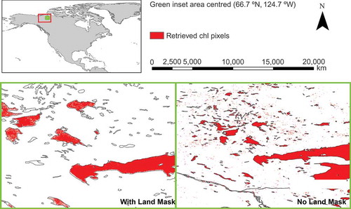
The water bodies resolvable from MERIS L2 imagery generated with and without the ODPS land/water mask (L2 Custom Processing, Figure 3) were compared for a sample area in the Canadian Shield to quantify the area of surface water that became visible by omitting the ODPS mask (see Figure 6). Of the ~700 water bodies determined from GLWD data to be present within the red box in the top panel of Figure 6, 65 were resolved from Level 2 MERIS imagery using the ODPS land mask, whereas 634 were resolved without the mask. The bottom panels of Figure 6 provide a closer view (corresponding to the green box) of the difference between the results using the NASA land/water mask (left) and using no mask (right). Removing the land/water mask does result in chl values being produced for some pixels outside of water bodies, which accounts for some of the speckling seen in the right inset image, but because we used the GLWD data as ‘ground truth’ for lake locations, this was not a concern for our purposes.

Figure 6. Comparison of chlorophyll estimates from MERIS L2 data for an area of the Canadian Shield (top panel). Of the ~700 water bodies present within the red box, 65 were resolved in an L2 image using the NASA ODPS land mask and 634 were resolved in the same image processed without the mask. For illustration, the area outlined in green in the top panel is shown in greater detail with the mask (below left) and without the mask (below right).

3.3. Description of 2011 snapshot data and global patterns

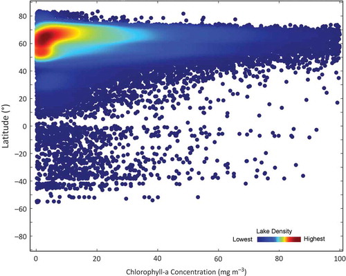
Using the new MTRI method with custom L2 processing on MERIS data, 1822 MERIS scenes were composited into a global growing season snapshot for 2011. Chl values could be retrieved for over 11 million 330 m pixels, representing a total surface area of ~1,228,000 km². The retrieved pixels represent 80,012 of the lakes defined in the GLWD shapefile (Figure 7), in sharp contrast to the 923 GLWD lakes that can be resolved from the L3 4 km MERIS OC4 product and the estimated 58,000 lakes that could have been resolved using the new MTRI method on MODIS 1 km imagery. The lakes that could be estimated using this new MERIS product represent approximately one-third of the 246,957 lakes ≥ 0.1 km² in the combined GLWD Levels 1 & 2 dataset. Figure 8 shows the distribution of lake-wide chl values for the lakes represented in the 2011 MERIS snapshot. Approximately 7% of all lakes were estimated to have extremely low chl values of less than 0.5 m⁻³, 28% had values of less than 5 mg m⁻³, 42% had mean values of less than 10 mg m⁻³, and 23% of all lakes had mean values exceeding 10 mg m⁻³. The mean chl for lakes visible in the MERIS composite was 19.2 ± 19.2, the median was 13.3, and the interquartile range was 3.90–28.6 mg m⁻³. Due to the uneven distribution of land on the Earth’s surface, the lakes retrieved in the northern hemisphere vastly outnumber those visible in the southern hemisphere (98.7% northern/1.3% southern). Figure 9 illustrates this; the concentration of points at mid-northern latitudes with medium to low chlorophyll-a values represents the chlorophyll-a distribution as well as the uneven distribution of fresh water on the Earth’s surface.

Figure 7. World distribution of the density of lakes from the GLWD shapefile and that are visible in the MERIS 2011 global snapshot composite when the land mask was not used for data processing. Lake densities are represented as the number of lakes whose centre points fall within 50 km of the pixel (an area of ~7850 km²). Note that lakes are heavily concentrated around 40–70° N.

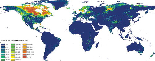
Figure 8. Histogram of mean lake-wide chl concentrations for the ~80,000 inland lakes from Global Lakes and Wetlands Database Levels 1 and 2 that could be retrieved with the MERIS 2011 global growing-season snapshot for world freshwater lakes. The mean chlorophyll-a value was 19.2 ± 19.2 mg m⁻³ and the median was 13.3 mg m^−3.

Figure 9. Density plot of mean lake-wide values of chl vs. the latitude of the lake’s centre point for the ~80,000 lakes resolvable in the MERIS global growing-season snapshot for the year 2011.

Table 2 presents the mean MERIS-derived chl estimates for different lake surface area size ranges. Though there is a general trend of decreasing chl with increasing surface area, the mean values for the four smallest size classes are fairly similar, with much lower mean values for only the very large lakes. This similarity indicates that without information on the drainage basin/lake area ratio, lake size alone is not a strong predictor of chl concentration at the global scale.

Table 2. Mean MERIS-derived chl estimates (mg m⁻³) from the 2011 global snapshot for different size ranges.

Surface area range (km^2)	Mean MERIS chl (mg m^−3)	Number of lakes
<1	19.1	9,743
1–10	19.5	58,087
10–100	17.9	10,839
100–1000	17.0	1,205
1000–10,000	14.1	121
>10,000	5.0	17
All lakes	19.2	80,012

Note: Number of lakes = global number of lakes in that size category represented in the 2011 global snapshot.

3.4. Comparison across ecoregions

3.4.1. Freshwater ecoregions of the world

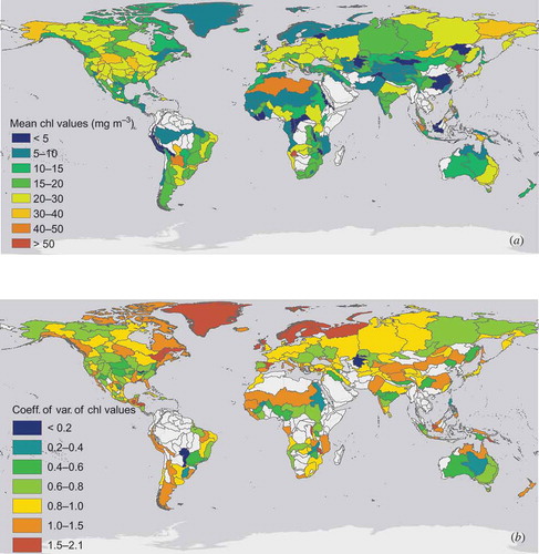
In order to evaluate whether the chl concentrations of lakes not visible to MERIS could be reasonably estimated based on their ecoregion, we examined the variation in lake chl values within and among biogeographic regions by calculating the mean value and coefficient of variation within each of Abell et al.’s (2008) Freshwater Ecoregions of the World (FEOW). FEOW polygons are delineated based on both hydrography and distinct biotic assemblages, using freshwater fish as a proxy. Though mean chl varied considerably among FEOW ecoregions, values were also highly variable within regions for much of the world (Figure 10). This high variability within ecoregions highlights the complexity of the factors determining the chl concentration of a given lake. Given these findings, the use of regional chl averages for further analysis does not appear to be very useful.

Figure 10. Mean MERIS-derived chl value (a) and coefficient of variation (CoV) (b) for each of Abell et al. (2008) Freshwater Ecoregions of the World. Light grey ecoregions include no retrieved lakes (a) or fewer than three retrieved lakes (b). The high CoV within many ecoregions indicates that lakes that are not retrieved by MERIS cannot be easily estimated based on their neighbours.

4. Discussion

4.1. Comparison to in situ data

The comparison of in situ and satellite chl estimates revealed some patterns for lake characteristics. Satellite chl estimates differed less from in situ values for larger lakes. In our validation, which included 37 lakes across the globe, the absolute difference between satellite and in situ chl estimates decreased with increasing lake size, but the percentage difference increased. Related to lake size, the absolute difference between in situ and satellite-derived chl values increased and the percentage difference decreased with increasing in situ trophic conditions. Chl values in larger lakes tend to be lower, but large lakes can also be highly heterogeneous (e.g. due to a eutrophic bay with much higher chl than the centre of the lake); this could potentially result in differences between in situ and satellite values depending on the sampling pattern used for the in situ measurements. In terms of the accuracy of satellite chlorophyll as a function of lake productivity, previous work indicates that satellites commonly overestimate chl in lakes with lower chl and underestimate chlorophyll in lakes with higher chl (Stramska et al. 2003; Cota, Wang, and Comiso 2004). Figure 5 largely confirmed this prediction, with the satellite estimate more frequently exceeding the in situ estimate for in situ chl values less than 5 mg m⁻³ and falling below it at high values.

When considering the comparisons between satellite and in situ estimates, however, several allowances regarding the in situ data should be noted. First, all of the in situ chl measurements used in the validation of the method presented here were originally collected by numerous researchers for varying purposes. The exact methods used to measure chl, the number of sampling sites used to generate the estimate and the distribution of those sites across the lake, and the number and timing of sample collections used to generate the estimates all varied among data sources, and for some lakes, some or all of these metadata were not reported. Thus, in some cases, the in situ measurements for a given lake and time span may not well represent the true mean near-surface chl concentration across the whole lake and time period. Non-representative in situ measurements likely contribute significantly to the difference observed between in situ and satellite-derived chl values. The good agreement between in situ and satellite-derived values, given this uncertainty, demonstrates the robustness of our approach. However, lacking a global database of standardized lake measurements, we aimed to assemble the best in situ dataset possible given the restrictions imposed by the use of MERIS data and the need to attempt to represent the global diversity of lakes.

Apart from the limitations of the in situ values themselves, the global in situ dataset compiled for this validation over-represents North America and its latitudes and ecoregions, as in situ chl measurements associated with explicit dates and lake location information were much more easily obtained for water bodies in North America than for much of the rest of the world. In particular, we found few suitable field data for South America and Africa, though as noted by Lehner and Döll (2004) and Verpoorter et al. (2014), the numbers of lakes on these continents greater than 1 km² are low relative to the mid-northern latitudes, contrasting with the prediction of Downing et al. (2006) based on a model of annual run-off.

4.2. Comparison of chl distributions for MERIS L3 product and new MTRI method

We compared the distribution of lake-wide chl concentrations produced with the new MTRI method, as shown in Figure 7, to the distribution of values produced with the MERIS OC4 L3 standard product for the same time periods. Both distributions were normalized by the total number of retrieved lakes. Compared with our global snapshot, the L3 product included a much higher proportion of low-chlorophyll (<5 mg m⁻³) lakes and lower proportion of higher-chl lakes (Figure 11). This is consistent with our expectation that because the L3 product represents only the largest lakes, it presents a lake distribution skewed towards low chl values. This comparison confirms that the new MTRI method produces a global distribution of lake chl values that is more accurate and representative of all lakes than readily available OC4 global composites.

Figure 11. Distributions of lake-wide chl values in the MTRI and NASA OceanColor L3 products for global summer 2011 (August for northern hemisphere lakes, February for southern hemisphere). Both histograms are normalized by the total number of lakes resolved in the respective products.

4.3. Lake detection limitations

The probability of retrieving chl estimates for a lake was inversely related to lake surface area for our global snapshot. This was expected, as the proportion of lakes presenting a contiguous area of surface water large enough to contain a MERIS pixel decreases with decreasing lake area. Significant proportions of all lake area classes in Figure 12 could not be retrieved by MERIS. These missing lakes include those that cannot be retrieved due to their shape (high shoreline development ratio), particularly impoundments, as well as the lakes for which there were no clear MERIS images in the month used for the global snapshot (August/February 2011 for the northern and southern hemispheres, respectively).

Figure 12. Percentage of lakes included in GLWD Levels 1 and 2 for which chl values could be retrieved from the 2011 growing-season global snapshot, separated into several lake surface area size classes.

Because we used the GLWD polygons to identify the locations of lakes, we are not able to estimate the number of lakes that are not included in our results because these are missing from the GLWD. Considering that the GLOWABO database (Verpoorter et al. 2014) includes roughly twice as many lakes >1 km² as the GLWD Levels 1 and 2 data utilized here, the number of lakes that could not be resolved because a better land mask than GLWD 1 and 2 was not available is presumably high. Most of the difference in the number of lakes included in GLWD and GLOWABO were in the 1–10 km² size range (~150,000 lakes in GLWD vs. 327,000 in GLOWABO). The future availability of GLOWABO or a similar product will therefore greatly increase the number of small lakes for which we can produce chl estimates.

The present work indicates that near-surface chl can be estimated from MERIS imagery for a large portion of lakes with surface area >4 km², as well as for thousands of lakes between ~1 and 4 km². Although our global snapshot does not indicate a clear relationship between lake size and chl concentration apart from our observation that very large lakes tended to be less productive, on average (Table 2) it remains possible that the lakes large enough to be resolvable in our dataset are not representative of the lakes <1 km² that could not be resolved. Lakes >1 km² do, however, represent a large fraction of total lake surface area (Verpoorter et al. 2014; Seekell et al. 2013), making unclear the importance of the bias in our snapshot caused by lake size constraints. In the future, availability of a satellite ocean colour sensor with a spatial resolution higher than MERIS would substantially improve the ability to monitor smaller inland lakes, among numerous other benefits.

In addition to inland lakes, our global snapshot also includes chl retrievals for many larger rivers of sufficient width to contain an unmixed water pixel (i.e. rivers of a Strahler order >5, where headwaters are assigned an order of 1 and the stream order increases when streams of the same order intersect; Strahler 1957). Although the total surface area of rivers (360,000 km² according to Lehner and Döll 2004, which is likely an underestimate) represents a small fraction of the total area of all inland waters relative to lakes, the importance of river fisheries can be disproportionately high in some regions (i.e. the Mississippi River in North America, the Amazon River in South America, the Mekong Delta in southeast Asia). As with very small lakes, finer-resolution imagery would be needed to retrieve chl values for most rivers due to their high shoreline development ratio.

Application of the new MTRI method to MERIS imagery throughout an entire year might provide significant insights into intra-annual global chl distribution variability, particularly in the northern latitudes (>50º N) where large differences in seasonal water temperature and ice cover duration may be important drivers of annual phytoplankton abundance and productivity. This is especially true when comparing temporally varying high-latitude production with more stable equatorial systems. Moreover, monthly global freshwater distributions of chl may provide observations of important episodic bloom events in remote lakes that are not captured in the ‘global summer’ composite nor are regularly sampled in the field.

4.4. Future potential of Landsat 8

Medium-resolution (~30 m) satellite missions (e.g. Landsat) offer the capability to observe lakes much smaller than the minimum mapping unit of traditional ocean colour missions; however, until the recent launch of Landsat 8, these platforms lacked the signal-to-noise ratios (SNR) (<100), spectral channels (440 nm), resolution (~100 nm band widths), and radiometric quantization (8-bit) to produce reliable chl estimates. The new Landsat 8 operational land imager (OLI) has an increased number (11) of narrow wavelength bands (20–50 nm), higher SNR (>200) and 12-bit quantization which support the retrieval of bio-geochemical properties, including surface chl concentrations (Pahlevan et al. 2014). Landsat 8 provides the potential to produce reliable and repeatable chl estimates for lakes as small as 0.002 km² (Verpoorter et al. 2014), which would further improve the estimate of global freshwater chl distribution. However, there are significant obstacles in generating a Landsat 8 global lake chl distribution including the acquisition of global cloud-free imagery, the relatively long temporal revisit (16 days), and massive computational overhead (1 GB file size per scene).

5. Conclusions

We demonstrated here that ocean colour satellite data can be used to generate reasonably robust estimates of lake-wide chlorophyll for a much larger proportion of freshwater lakes (at least ~1 km² in area) than has previously been assumed. Worldwide, the mean estimated lake-wide chlorophyll-a value during the 2011 growing season was 19.2 ± 19.2 mg m⁻³ and the median was 13.3 mg m⁻³. The existing NASA Level 2 and Level 3 OceanColor products for MODIS and MERIS were not suitable for generating a global snapshot of freshwater chl due to the land mask used in Level 2 processing and the reduced resolution of Level 3 products. By processing MERIS OC4 Level 1A data to Level 2 without use of the land/water mask and then compositing that imagery to a global 330 m product, we were able to produce estimates of the growing-season chl concentration in 2011 for a much larger number of freshwater lakes. This global dataset will serve as a valuable input for future work, such as producing global extrapolations of inland fisheries’ harvest and primary production in inland waters.

Disclosure statement

No potential conflict of interest was reported by the authors.

ORCID

Robert A. Shuchman http://orcid.org/0000-0002-6097-4945

Acknowledgements

Data were provided by the European Space Agency. The authors express their appreciation to Scott Hawkins for assistance with data processing. This article is Contribution 1920 of the US Geological Survey Great Lakes Science Center. Any use of trade, product, or firm names is for descriptive purposes only and does not imply endorsement by the US Government.

Additional information

Funding

This work was supported by the US Geological Survey under Grant G12AC20299.

References

- Abell, R., M. L. Thieme, C. Revenga, M. Bryer, M. Kottelat, N. Bogutskaya, B. Coad, N. Mandrak, S. Contreras Balderas, W. Bussing, M. L. J. Stiassny, P. Skelton, G. R. Allen, P. Unmack, A. Naseka, R. Ng, N. Sindorf, J. Robertson, R. Armijo, J. V. Higgins, T. J. Heibel, R. Wikramanayake, D. Olson, H. L. López, R. E. Reis, J. G. Lundberg, M. H. Sabaj Pérez, and P. Petry. 2008. “Freshwater Ecoregions of the World: A New Map of Biogeographic Units for Freshwater Biodiversity Conservation.” BioScience 58 (5): 403–414. doi:10.1641/B580507.
- Adrian, R., C. M. O’Reilly, H. Zagarese, S. B. Baines, D. O. Hessen, W. Keller, D. M. Livingstone, R. Sommaruga, D. Straile, E. Van Donk, G. A. Weyhenmeyer, and M. Winder. 2009. “Lakes as Sentinels of Climate Change.” Limnology and Oceanography 54 (6, Part 2): 2283–2297. doi:10.4319/lo.2009.54.6_part_2.2283.
- ALMS (Alberta Lake Management Society). 2008. The Alberta Lake Management Society Volunteer Lake Monitoring Report: Amisk Lake. Edmonton: Alberta Lake Management Society.
- Barus, T. A., S. S. Sinaga, and R. Tarigan. 2008. “Phytoplankton Primary Productivity Linked to Physical-Chemical Factors Water in Water Parapat, Lake Toba.” Biological Journal of University of North Sumatra 3 (1): 11–16.
- Binding, C. E., T. Greenberg, and R. P. Bukata. 2012. “An Analysis of MODIS-Derived Algal and Mineral Turbidity in Lake Erie.” Journal of Great Lakes Research 38 (1): 107–116. doi:10.1016/j.jglr.2011.12.003.
- Bukata, R. P. 2005. Satellite Monitoring of Inland and Coastal Water Quality: Retrospection, Introspection, Future Directions. Boca Raton, FL: CRC Press.
- Campbell, G., S. R. Phinn, A. G. Dekker, and V. E. Brando. 2011. “Remote Sensing of Water Quality in an Australian Tropical Freshwater Impoundment Using Matrix Inversion and MERIS Images.” Remote Sensing of Environment 115 (9): 2402–2414. doi:10.1016/j.rse.2011.05.003.
- Campbell, I. C., C. Poole, W. Giesen, and J. Valbo-Jorgensen. 2006. “Species Diversity and Ecology of Tonle Sap Great Lake, Cambodia.” Aquatic Sciences 68: 355–373. doi:10.1007/s00027-006-0855-0.
- Chavula, G., P. Brezonik, P. Thenkabail, T. Johnson, and M. Bauer. 2009. “Estimating Chlorophyll Concentration in Lake Malawi from MODIS Satellite Imagery.” Physics and Chemistry of the Earth, Parts A/B/C 34 (13–16): 755–760. doi:10.1016/j.pce.2009.07.015.
- Cole, J. J., Y. T. Prairie, N. F. Caraco, W. H. McDowell, L. J. Tranvik, R. G. Striegl, C. M. Duarte, P. Kortelainen, J. A. Downing, J. J. Middelburg, and J. Melack. 2007. “Plumbing the Global Carbon Cycle: Integrating Inland Waters into the Terrestrial Carbon Budget.” Ecosystems 10 (1): 172–185. doi:10.1007/s10021-006-9013-8.
- Cota, G. F., J. Wang, and J. C. Comiso. 2004. “Transformation of Global Satellite Chlorophyll Retrievals with a Regionally Tuned Algorithm.” Remote Sensing of Environment 90 (3): 373–377. doi:10.1016/j.rse.2004.01.005.
- De Moraes Novo, E. M. L., C. C. De Farias Barbosa, R. M. De Freitas, Y. E. Shimabukuro, J. M. Melack, and W. Pereira Filho. 2006. “Seasonal Changes in Chlorophyll Distributions in Amazon Floodplain Lakes Derived from MODIS Images.” Limnology 7 (3): 153–161. doi:10.1007/s10201-006-0179-8.
- Doerffer, R., K. Sorensen, and J. Aiken. 1999. “MERIS Potential for Coastal Zone Applications.” International Journal of Remote Sensing 20: 1809–1818. doi:10.1080/014311699212498.
- Downing, J. A., Y. T. Prairie, J. J. Cole, C. M. Duarte, L. J. Tranvik, R. G. Striegl, W. H. McDowell, P. Kortelainen, N. F. Caraco, J. M. Melack, and J. J. Middelburg. 2006. “The Global Abundance and Size Distribution of Lakes, Ponds, and Impoundments.” Limnology and Oceanography 51 (5): 2388–2397. doi:10.4319/lo.2006.51.5.2388.
- Dudgeon, D., A. H. Arthington, M. O. Gessner, Z. I. Kawabata, D. J. Knowler, C. Lévêque, R. J. Naiman, A. Prieur-Richard, D. Soto, M. L. J. Stiassny, and C. A. Sullivan. 2006. “Freshwater Biodiversity: Importance, Threats, Status and Conservation Challenges.” Biological Reviews 81 (2): 163–182. doi:10.1017/S1464793105006950.
- Ficke, A. D., C. A. Myrick, and L. J. Hansen. 2007. “Potential Impacts of Global Climate Change on Freshwater Fisheries.” Reviews in Fish Biology and Fisheries 17 (4): 581–613. doi:10.1007/s11160-007-9059-5.
- Franz, B. 2013. “NASA Satellite Ocean Color Timeseries.” Paper presented at the International Ocean Color Science Meeting, Darmstadt, May 6–8.
- Garno, Y. S. 2003. “Reservoir Water Quality Status, Juanda.” Journal of Technology Environment 4 (3): 128–135.
- Gitelson, A. A., D. Gurlin, W. J. Moses, and T. Barrow. 2009. “A Bio-Optical Algorithm for the Remote Estimation of the Chlorophyll-A Concentration in Case 2 Waters.” Environmental Research Letters 4 (4): 045003. doi:10.1088/1748-9326/4/4/045003.
- Gons, H. J., M. T. Auer, and S. W. Effler. 2008. “MERIS Satellite Chlorophyll Mapping of Oligotrophic and Eutrophic Waters in the Laurentian Great Lakes.” Remote Sensing of Environment 112 (11): 4098–4106. doi:10.1016/j.rse.2007.06.029.
- Gons, H. J., M. Rijkeboer, and K. G. Ruddick. 2002. “A Chlorophyll-Retrieval Algorithm for Satellite Imagery (Medium Resolution Imaging Spectrometer) of Inland and Coastal Waters.” Journal of Plankton Research 24 (9): 947–951. doi:10.1093/plankt/24.9.947.
- Gons, H. J., M. Rijkeboer, and K. G. Ruddick. 2005. “Effect of a Waveband Shift on Chlorophyll Retrieval from MERIS Imagery of Inland and Coastal Waters.” Journal of Plankton Research 27 (1): 125–127. doi:10.1093/plankt/fbh151.
- Gower, J. F. R., R. Doerffer, and G. A. Borstad. 1999. “Interpretation of the 685nm Peak in Water-Leaving Radiance Spectra in Terms of Fluorescence, Absorption and Scattering, and Its Observation by MERIS.” International Journal of Remote Sensing 20: 1771–1786. doi:10.1080/014311699212470.
- Heim, B., H. Oberhaensli, S. Fietz, and H. Kaufmann. 2005. “Variation in Lake Baikal’s Phytoplankton Distribution and Fluvial Input Assessed by SeaWiFS Satellite Data.” Global and Planetary Change 46: 9–27. doi:10.1016/j.gloplacha.2004.11.011.
- Hu, C., Z. Lee, and B. Franz. 2012. “Chlorophyll A Algorithms for Oligotrophic Oceans: A Novel Approach Based on Three-Band Reflectance Difference.” Journal of Geophysical Research 117: C01011. doi:10.1029/2011JC007395.
- Kallio, K., T. Kutser, T. Hannonen, S. Koponen, J. Pulliainen, J. Vepsäläinen, and T. Pyhälahti. 2001. “Retrieval of Water Quality from Airborne Imaging Spectrometry of Various Lake Types in Different Seasons.” Science of the Total Environment 268 (1–3): 59–77. doi:10.1016/S0048-9697(00)00685-9.
- Khondker, M., A. Alfasane, A. Gani, and S. Islam. 2012. “Limnological notes on Ramsagar, Dinajpur, Bangladesh.” Bangladesh Journal of Botany 41 (1): 119–121. doi:10.3329/bjb.v41i1.11091.
- Koponen, S., K. Kallio, J. Pulliainen, J. Vepsalainen, T. Pyhalahti, and M. Hallikainen. 2004. “Water Quality Classification of Lakes Using 250-M MODIS Data.” IEEE Geoscience and Remote Sensing Letters 1: 287–291. doi:10.1109/LGRS.2004.836786.
- Korosov, A. A., D. V. Pozdnyakov, A. Folkestad, L. H. Pettersson, K. Sørensen, and R. Shuchman. 2009. “Semi-Empirical Algorithm for the Retrieval of Ecology-Relevant Water Constituents in Various Aquatic Environments.” Algorithms 2: 470–497. doi:10.3390/a2010470.
- Lee, Z., K. L. Carder, and R. A. Arnone. 2002. “Deriving Inherent Optical Properties from Water Color: A Multiband Quasi-Analytical Algorithm for Optically Deep Waters.” Applied Optics 41 (27): 5755–5772. doi:10.1364/AO.41.005755.
- Lee, Z. P., ed. 2006. Remote Sensing of Inherent Optical Properties: Fundamentals, Tests of Algorithms, and Applications. Reports of the International Ocean-Colour Coordinating Group No. 5. Dartmouth: IOCCG.
- Lehner, B., and P. Döll. 2004. “Development and Validation of a Global Database of Lakes, Reservoirs and Wetlands.” Journal of Hydrology 296 (1–4): 1–22. doi:10.1016/j.jhydrol.2004.03.028.
- Lesht, B. M., R. P. Barbiero, and G. J. Warren. 2012. “Satellite Ocean Color Algorithms: A Review of Applications to the Great Lakes.” Journal of Great Lakes Research 38 (1): 49–60. doi:10.1016/j.jglr.2011.10.005.
- Lyche-Solheim, A., C. K. Feld, S. Birk, G. Phillips, L. Carvalho, G. Morabito, U. Mischke, N. Willby, M. Søndergaard, S. Hellsten, A. Kolada, M. Mjelde, J. Böhmer, O. Miler, M. T. Pusch, C. Argillier, E. Jeppesen, T. L. Lauridsen, and S. Poikane. 2013. “Ecological Status Assessment of European Lakes: A Comparison of Metrics for Phytoplankton, Macrophytes, Benthic Invertebrates and Fish.” Hydrobiologia 704 (1): 57–74. doi:10.1007/s10750-012-1436-y.
- Maritorena, S., D. A. Siegel, and A. R. Peterson. 2002. “Optimization of a Semianalytical Ocean Color Model for Global-Scale Applications.” Applied Optics 41: 2705–2714. doi:10.1364/AO.41.002705.
- Matthews, M. W. 2011. “A Current Review of Empirical Procedures of Remote Sensing in Inland and Near-Coastal Transitional Waters.” International Journal of Remote Sensing 32 (21): 6855–6899. doi:10.1080/01431161.2010.512947.
- Morel, A., and L. Prieur. 1977. “Analysis of Variations in Ocean Color.” Limnology and Oceanography 22 (4): 709–722. doi:10.4319/lo.1977.22.4.0709.
- Moses, W. J., A. A. Gitelson, S. Berdnikov, and V. Povazhnyy. 2009. “Satellite Estimation of Chlorophyll-a Concentration Using the Red and NIR Bands of MERIS—The Azov Sea Case Study.” IEEE Geoscience and Remote Sensing Letters 6 (4): 845–849. doi:10.1109/LGRS.2009.2026657.
- NASA (National Aeronautics and Space Administration). 2010. Ocean Level-2 Data Products March 22, 2010, Ocean Color Web. Accessed January 11, 2011. http://oceancolor.gsfc.nasa.gov/DOCS/Ocean_Level-2_Data_Products.pdf
- Nemirovskaya, I. A. 2012. “Variations in Different Compounds in Volga Water, Suspension, and Bottom Sediments in the Summer of 2009.” Water Resources 39 (5): 533–545. doi:10.1134/S0097807812030062.
- Niksic, H. 1998. GNU Wget. http://www.gnu.org/software/wget/
- O’Reilly, J., S. Maritorena, M. O’Brien, D. Siegel, D. Toole, D. Menzies, R. Smith, J. L. Mueller, B. G. Mitchell, M. Kahru, F. P. Chavez, P. Strutton, G. F. Cota, S. B. Hooker, C. R. McClain, K. L. Carder, F. Müller-Karger, L. Harding, A. Magnuson, D. Phinney, G. F. Moore, J. Aiken, K. R. Arrigo, R. Letelier, and M. Culver. 2000. SeaWiFS Postlaunch Calibration and Validation Analyses, Part 3. Vol 11 of NASA Technical Memorandum 2000-206892. Edited by S. B. Hooker and E. R. Firestone. Greenbelt, MD: Goddard Space Flight Center.
- O’Reilly, J. E., S. Maritorena, B. G. Mitchell, D. A. Siegel, K. L. Carder, S. A. Garver, M. Kahru, and C. McClain. 1998. “Ocean Color Chlorophyll Algorithms for SEAWIFS.” Journal of Geophysical Research: Oceans 103 (C11): 24937–24953. doi:10.1029/98JC02160.
- Odermatt, D., T. Heege, J. Nieke, M. Kneubühler, and K. Itten. 2008. “Water Quality Monitoring for Lake Constance with a Physically Based Algorithm for MERIS Data.” Sensors 8 (8): 4582–4599. doi:10.3390/s8084582.
- Pahlevan, N., Z. Lee, J. Wei, C. B. Schaaf, J. R. Schott, and A. Berk. 2014. “On-Orbit Radiometric Characterization of OLI (Landsat-8) for Applications in Aquatic Remote Sensing.” Remote Sensing of Environment 154: 272–284. doi:10.1016/j.rse.2014.08.001.
- Palmer, S. C. J., T. Kutser, and P. D. Hunter. 2015. “Remote Sensing of Inland Waters: Challenges, Progress and Future Directions.” Remote Sensing of Environment 157: 1–8. doi:10.1016/j.rse.2014.09.021.
- Piccini, C., D. Conde, C. Alonso, R. Sommaruga, and J. Pernthaler. 2006. “Blooms of Single Bacterial Species in a Coastal Lagoon of the Southwestern Atlantic Ocean.” Applied and Environmental Microbiology 72 (10): 6560–6568. doi:10.1128/AEM.01089-06.
- Pla, S., A. M. Paterson, J. P. Smol, B. J. Clark, and R. Ingram. 2005. “Spatial Variability in Water Quality and Surface Sediment Diatom Assemblages in a Complex Lake Basin: Lake of the Woods, Ontario, Canada.” Journal of Great Lakes Research 31: 253–266. doi:10.1016/S0380-1330(05)70257-4.
- Revenga, C., I. Campbell, R. Abell, P. De Villiers, and M. Bryer. 2005. “Prospects for Monitoring Freshwater Ecosystems Towards the 2010 Targets.” Philosophical Transactions of the Royal Society B 360 (1454): 397–413.
- Sathyendranath, S., ed. 2000. Remote Sensing of Ocean Colour in Coastal, and Other Optically Complex, Waters. Reports of the International Ocean-Colour Coordinating Group No. 3. Dartmouth: IOCCG.
- Schindler, E., K. Ashley, R. Rae, L. Vidmanic, H. Andrusak, D. Sebastian, G. Scholten, P. Woodruff, F. Pick, L. M. Ley, and P. B. Hamilton. 2006. “Kootenay Lake Fertilization Experiment; Years 11 and 12.” 2002–2003 Technical Report. Project No. 199404900. 207 electronic pages, (BPA Report DOE/BP-00004029-5).
- Seekell, D. A., M. L. Pace, L. J. Tranvik, and C. Verpoorter. 2013. “A Fractal-Based Approach to Lake Size Distributions.” Geophysical Research Letters 40 (3): 517–521. doi:10.1002/grl.50139.
- Shuchman, R. A., G. Leshkevich, M. J. Sayers, T. H. Johengen, C. N. Brooks, and D. Pozdnyakov. 2013. “An Algorithm to Retrieve Chlorophyll, Dissolved Organic Carbon, and Suspended Minerals from Great Lakes Satellite Data.” Journal of Great Lakes Research 39: 14–33. doi:10.1016/j.jglr.2013.06.017.
- Simis, S. G. H., A. Ruiz-Verdú, J. A. Domínguez-Gómez, R. Peña-Martinez, S. W. M. Peters, and H. J. Gons. 2007. “Influence of Phytoplankton Pigment Composition on Remote Sensing of Cyanobacterial Biomass.” Remote Sensing of Environment 106: 414–427. doi:10.1016/j.rse.2006.09.008.
- Soares, M. C. S., M. I. De A Rocha, M. M. Marinho, S. M. F. O. Azevedo, C. W. Branco, and V. L. Huszar. 2009. “Changes in Species Composition during Annual Cyanobacterial Dominance in a Tropical Reservoir: Physical Factors, Nutrients and Grazing Effects.” Aquatic Microbial Ecology 57 (2): 137–149. doi:10.3354/ame01336.
- Strahler, A. N. 1957. “Quantitative Analysis of Watershed Geomorphology.” Eos, Transactions American Geophysical Union 38 (6): 913–920. doi:10.1029/TR038i006p00913.
- Stramska, M., D. Stramski, R. Hapter, S. Kaczmarek, and J. Stoń. 2003. “Bio-Optical Relationships and Ocean Color Algorithms for the North Polar Region of the Atlantic.” Journal of Geophysical Research: Oceans 108: C5. doi:10.1029/2001JC001195.
- Strayer, D. L. 2010. “Alien Species in Fresh Waters: Ecological Effects, Interactions with Other Stressors, and Prospects for the Future.” Freshwater Biology 55 (s1): 152–174. doi:10.1111/j.1365-2427.2009.02380.x.
- Van Der Sande, C., N. Van De Giesen, K. Poser, and S. Peters. 2012. EO Information Services in support of Zambezi River Basin Mapping. Lusaka: Water Board.
- Verpoorter, C., T. Kutser, D. A. Seekell, and L. J. Tranvik. 2014. “A Global Inventory of Lakes Based on High-Resolution Satellite Imagery.” Geophysical Research Letters 41 (18): 6396–6402. doi:10.1002/2014GL060641.
- Viljanen, M., V. Drabkova, V. Avinsky, L. Kapustina, and G. Raspletina. 2008. “Ecological State and Monitoring of Limnological and Biological Parameters in Lake Ladoga, Russia.” Aquatic Ecosystem Health & Management 11 (1): 61–74. doi:10.1080/14634980801891548.
- Vitousek, P. M., H. A. Mooney, J. Lubchenco, and J. M. Melillo. 1997. “Human Domination of Earth’s Ecosystems.” Science 277: 494–499. doi:10.1126/science.277.5325.494.
- Vos, R. J., J. H. M. Hakvoort, R. W. J. Jordans, and B. W. Ibelings. 2003. “Multiplatform Optical Monitoring of Eutrophication in Temporally and Spatially Variable Lakes.” Science of the Total Environment 312 (1–3): 221–243. doi:10.1016/S0048-9697(03)00225-0.
- Welcomme, R. L. 2011. “An Overview of Global Catch Statistics for Inland Fish.” ICES Journal of Marine Science 68 (8): 1751–1756. doi:10.1093/icesjms/fsr035.
- Wilson, M. A., and S. R. Carpenter. 1999. “Economic Valuation of Freshwater Ecosystem Services in the United States: 1971–1997.” Ecological Applications 9 (3): 772–783.
- Wondie, A., S. Mengistu, J. Vijverberg, and E. Dejen. 2007. “Seasonal Variation in Primary Production of a Large High Altitude Tropical Lake (Lake Tana, Ethiopia): Effects of Nutrient Availability and Water Transparency.” Aquatic Ecology 41 (2): 195–207. doi:10.1007/s10452-007-9080-8.
- Wu, M., W. Zhang, X. Wang, and D. Luo. 2009. “Application of MODIS Satellite Data in Monitoring Water Quality Parameters of Chaohu Lake in China.” Environmental Monitoring and Assessment 148 (1–4): 255–264. doi:10.1007/s10661-008-0156-2.
- Yang, L., K. Lei, W. Meng, G. Fu, and W. Yan. 2013. “Temporal and Spatial Changes in Nutrients and Chlorophyll-Α in a Shallow Lake, Lake Chaohu, China: An 11-Year Investigation.” Journal of Environmental Sciences 25 (6): 1117–1123. doi:10.1016/S1001-0742(12)60171-5.
- Yentsch, C. S. 1960. “The Influence of Phytoplankton Pigments on the Colour of Sea Water.” Deep Sea Research (1953) 7 (1): 1–9. doi:10.1016/0146-6313(60)90002-2.
- Zhang, Y. L., B. Q. Qin, and M. L. Liu. 2007. “Temporal-Spatial Variations of Chlorophyll a and Primary Production in Meiliang Bay, Lake Taihu, China from 1995 to 2003.” Journal of Plankton Research 29 (8): 707–719. doi:10.1093/plankt/fbm049.