Differentiating mine-reclaimed grasslands from spectrally similar land cover using terrain variables and object-based machine learning classification

Abstract

Incorporating ancillary, non-spectral data may improve the separability of land use/land cover classes. This study investigates the use of multi-temporal digital terrain data combined with aerial National Agriculture Imagery Program imagery for differentiating mine-reclaimed grasslands from non-mining grasslands across a broad region (6085 km²). The terrain data were derived from historical digital hypsography and a recent light detection and ranging data set. A geographic object-based image analysis (GEOBIA) approach, combined with two machine learning algorithms, Random Forests and Support Vector Machines, was used because these methods facilitate the use of ancillary data in classification. The results suggest that mine-reclaimed grasslands can be mapped accurately, with user’s and producer’s accuracies above 80%, due to a distinctive topographic signature in comparison with other spectrally similar grasslands within this landscape. The use of multi-temporal digital elevation model data and pre-mining terrain data only generally provided statistically significant increased classification accuracy in comparison with post-mining terrain data. Elevation change data were of value, and terrain shape variables generally improved the classification. GEOBIA and machine learning algorithms were useful in exploiting these non-spectral data, as data gridded at variable cell sizes can be summarized at the scale of image objects, allowing complex interactions between predictor variables to be characterized.

1. Introduction

Mapping land use change is important for studies of anthropogenic global change (Anderson et al. 1976; Folke et al. 2007; Cihlar and Jansen 2001). Nevertheless, some land-use/land-cover (LULC) classes may not be spectrally distinctive, resulting in low classification accuracy when multispectral data are used to produce a thematic map. This is especially true when attempting to map land-use classes, since the use of land does not necessarily result in spectrally distinctive properties. Ancillary, non-spectral data may help differentiate these spectrally similar LULC classes (Gislason, Benediktsson, and Sveinsson 2006; Treitz and Howarth 2000; Knight et al. 2013).

Mine reclamation is an example of a land use that may not be spectrally distinguishable in aerial and satellite imagery. Mountaintop removal with valley fills (MTR/VF) mining is a resource extraction approach practised in the Appalachian region of the United States of America (USA), especially in southern West Virginia, eastern Kentucky, and southwestern Virginia. In this region, heavy machinery and explosives are used to expose coal seams of the Pennsylvanian geologic subperiod. MTR/VF mining results in faster and more pervasive terrain alteration than more traditional mining techniques (Fritz et al. 2010). Excavation and the subsequent reclamation associated with MTR/VF results in considerable physical terrain alteration, as 50–200 m of rock material is commonly removed from mountaintops and the unconsolidated rock waste is disposed of in the adjacent valleys as so-called valley fills, filling headwater streams and generally raising valley elevations (Hooke 1994, 1999; Fritz et al. 2010; Palmer et al. 2010; Bernhardt and Palmer 2011; Bernhardt et al. 2012; Maxwell and Strager 2013). This practice alters the pre-mining landforms of the affected mountaintops and valleys, flattening the upper slopes of a landscape that was originally characterized by moderate to strong relief and steep slopes dissected by a dendritic stream network (Ehlke, Runner, and Downs 1982; Maxwell and Strager 2013). The resulting topographically altered terrain, which was generally forested before mining, is commonly reclaimed to grasslands or shrublands (Simmons et al. 2008; Kazar and Warner 2013). Because this mining practice results in such characteristic topographic alteration, multi-temporal terrain data may facilitate the differentiation of MTR/VF reclaimed grasslands from other spectrally similar grasslands within this landscape.

In this article, we explore the use of multi-temporal, digital elevation model (DEM)-derived terrain data combined with high-resolution aerial orthophotography for differentiating mine-reclaimed grasslands from other grasslands. The study site comprises three watersheds covering 6085 km² in West Virginia, USA, a region where extensive landscape alteration has taken place due to surface coal mining, especially MTR/VF. A geographic object-based image analysis (GEOBIA) approach and machine learning algorithms are used to integrate the disparate data at differing scales. The following research questions are addressed:

1. Can mine-reclaimed grasslands be separated from other grasslands across broad regions using DEM-derived terrain characteristics?

2. Is it necessary to use both pre- and post-mining terrain characteristics to obtain an accurate separation of these classes? Or, can an accurate separation be obtained using only topography from a single time period (e.g. the current landscape)?

3. Do derived terrain attributes help differentiate these grassland classes, and, if so, what terrain attributes are most important?

2. Background

2.1. Importance of mapping mine-reclaimed grasslands

Grasslands resulting from surface mine reclamation have been shown to be fundamentally different from other grasslands in terms of their impact on hydrology (Negley and Eshleman 2006; Ferrari et al. 2009; McCormick et al. 2009; Zégre, Maxwell, and Lamont 2013; Miller and Zégre 2014; Zégre et al. 2014), terrestrial habitat (Weakland and Wood 2005; Wood, Bosworth, and Dettmers 2006; Simmons et al. 2008; Wickham et al. 2007, 2013), and aquatic ecosystems (Hartman et al. 2005; Pond et al. 2008; Fritz et al. 2010; Pond 2010; Merriam et al. 2011; Bernhardt et al. 2012; Merriam et al. 2013). Negley and Eshleman (2006) found that watersheds affected by mining and mine reclamation produce increased storm run-off and higher peak hourly run-off rates for storm events in comparison with watersheds not affected by mining. These observations were attributed to the loss of tree canopy and reduced evapotranspiration, as well as decreased infiltration due to soil compaction. However, in a review of the hydrologic impacts of MTR/VF mining and mine reclamation, Miller and Zégre (2014) suggest that the hydrology of such systems is not well understood. Although traditional mining practices generally increase peak and total run-off, the hydrologic impacts of MTR/VF reclamation are confounded by the increased storage of water in valley fill spoil and the reduced infiltration resulting from the compaction of soils above the fill.

Concerning the effect on terrestrial habitats, Wood, Bosworth, and Dettmers (2006) suggest that mine reclamation and loss of forest negatively affect Cerulean Warbler (Dendroica cerulea) populations, a species of conservation concern. Simmons et al. (2008) document nutrient limitations within terrestrial ecosystems impacted by mine reclamation that may persist for decades or centuries. Within aquatic ecosystems, Pond (2010) found that the number and richness of assemblages of mayflies (Ephemeroptera), especially sensitive aquatic insect taxa, were reduced in streams impaired by mining in comparison with reference sites. Merriam et al. (2013) found a direct correlation between selenium (Se) concentrations in streams and the extent of surface mining and reclamation upstream. Thus, because mine reclamation has unique and profound impacts on hydrological processes, terrestrial habitat, and aquatic ecosystems, it is important to be able to map and differentiate such land use from spectrally similar classes. In particular, information on the extent and location within the modified topographic landscape of reclaimed grasslands is a foundational data layer for environmental studies of MTR/VF landscapes.

2.2. Terrain data for mapping and modelling

Terrain data have been integrated into LULC mapping in many previous studies to improve classification accuracy. For example, Gislason, Benediktsson, and Sveinsson (2006) combined elevation, topographic slope, and topographic aspect derived from DEM data with Landsat Multispectral Scanner (MSS) data for mapping forest types in Colorado, USA, and noted the value of elevation in the classification. Treitz and Howarth (2000) found that DEM data improved classification accuracy for forest ecosystems in northern Ontario, Canada. Although terrain information alone provided a weak separation of the forest ecosystem classes, combining these data with spectral data improved the classification. Knight et al. (2013) also noted an improvement in classification accuracy when topographic derivatives such as compound topographic moisture index (CTMI), topographic slope, and slope curvature were combined with spectral data for mapping palustrine wetlands. Terrain data have also been used as predictor variables for spatial modelling (for example, Prasad, Iverson, and Liaw 2006; Wright and Gallant 2007; Pino-Mejías et al. 2010; Evans and Kiesecker 2014). However, a review of the current literature suggests that multi-temporal terrain data have not been explored for mapping LULC classes within landscapes characterized by extensive anthropogenic topographic alteration.

2.3. Mapping surface mining and reclamation

Because mine reclamation generally persists as a legacy landscape alteration, mapping reclamation is of particular interest. However, as Rathore and Wright (1993) note, mine reclamation has proven more difficult to map than active mining. Research investigating the mapping of LULC resulting from mining and mine reclamation has traditionally focused on moderate spatial resolution multispectral data, such as MSS, Thematic Mapper (TM), Enhanced Thematic Mapper Plus (ETM+), and Satellite Pour l’Observation de la Terre (SPOT) data (Irons and Kennard 1986; Parks, Petersen, and Baumer 1987; Rathore and Wright 1993; Anderson et al. 1997; Prakash and Gupta 1998; Townsend et al. 2009; Sen et al. 2012). In contrast, our previous research has explored the use of high-spatial-resolution satellite and aerial data, the combination of spectral and light detection and ranging (lidar) data, and the implementation of GEOBIA and machine learning algorithms for mapping mining and mine reclamation at the scale of a single mine (Maxwell et al. 2014a, 2014b, 2015). This research expands upon our previous work by focusing particularly on the potential benefit of multi-temporal terrain data, integrated with high-resolution aerial imagery, for differentiating mine-reclaimed grasslands for regional mapping of reclamation. Indeed, to our knowledge, this is the first study on mapping grasslands associated with mine reclamation at a fine resolution (5 m) across a broad region.

A notable example of previous mapping of mining and mining reclamation with moderate scale data is the work of Townsend et al. (2009), who mapped mining and mine reclamation across a region encompassing eight river basins in the Central Appalachian Mountain region of the Eastern United States. Four Landsat MSS, TM, and ETM+ scenes from 1976, 1987, 1999, and 2006 were classified to map spectrally separable land cover classes. They then developed a decision tree process utilizing characteristic transitions of land cover to separate mining and mine reclamation from other classes within a mine mask. Accuracies for mapping mining and mine reclamation were generally above 85% using this method. Sen et al. (2012) expanded upon this work using a time series of Landsat TM and ETM+ data to differentiate re-vegetated mines from other forest-displacing disturbance such as urbanization, using disturbance and subsequent recovery trajectories and a GEOBIA approach across four counties impacted by MTR/VF mining in southwestern Virginia. An accuracy of 89% was obtained.

These previous studies suggest that reclaimed mine lands can be separated from spectrally similar land cover using multi-temporal data. However, a time series is not commonly available when working with high-resolution satellite or aerial data, suggesting that other methods must be explored if mapping is to be undertaken at a high spatial resolution.

2.4. GEOBIA and machine learning algorithms

GEOBIA, the process of segmenting an image into objects, or contiguous groups of pixels that are relatively spectrally homogeneous and labelling each resulting object as a single unit, has been described as a paradigm shift in remote sensing (Blaschke et al. 2014). GEOBIA has been shown to be particularly applicable for the classification of high-spatial-resolution data (Blaschke and Strobl 2001; Walter 2004; Chubey, Franklin, and Wulder 2006; Drăguţ and Blaschke 2006; Blaschke 2010; Baker et al. 2013). A feature of GEOBIA of great significance for incorporating information from ancillary layers is that the spatial support (i.e. data structure and resolution) of the ancillary data does not need to be the same as the pixel grid used to develop the objects.

Once image objects are produced, a wide variety of summary spectral (e.g. mean, standard deviation (std), range, minimum (min), maximum (max) of image bands) and spatial (e.g. shape, size, and association with neighbouring objects) properties can be summarized for each object (Trimble 2011). However, many of these variables may not meet the assumptions of multivariate normality required for statistical classifiers and, as a result, nonparametric, machine learning approaches are commonly used in GEOBIA (Ke, Quackenbush, and Im 2010; Trimble 2011; Duro, Franklin, and Dubé 2012a, 2012b). Machine learning algorithms offer the potential to handle high-dimensional complex spectral measurement spaces and large volumes of data, with the added benefit of reduced processing time compared with traditional classifiers (Hansen and Reed 2000). In this study, two machine learning algorithms were used, Support Vector Machines (SVM) (Vapnik 1995; Joachims 1998; Burges 1998; Tso and Mather 2003; Pal and Mather 2005; Pal 2005; Warner and Nerry 2009) and Random Forests (RF) (Breiman 2001).

SVMs separate two classes by constructing a multi-dimensional hyperplane that is optimized as the maximum margin that provides the best separation between the classes. To create this decision boundary, it is usually necessary to transform the data to a higher-dimensional space in order for the data to be linearly separable. This is accomplished using a kernel function, such as a polynomial or radial basis function (RBF). To facilitate generalization of the decision boundary, a penalty parameter (C) penalizes training samples located on the ‘wrong’ side of the decision boundary (Vapnik 1995; Joachims 1998; Burges 1998; Tso and Mather 2003; Pal and Mather 2005; Pal 2005; Warner and Nerry 2009). SVM algorithms were originally designed for two class problems and, as a result, strategies are required to allow for the separation of more than two classes. For example, the ‘one-against-one’ approach uses binary classifiers and a voting scheme to separate multiple classes (Vapnik 1995; Tso and Mather 2003; Pal 2005; Pal and Mather 2005; Meyer et al. 2012).

RF uses an ensemble of classification trees to improve upon the accuracy and consistency of single decision tree (DT) classifications. RF differs from other ensemble DT methods because each tree is generated from a subsample of the data obtained from random bootstrap sampling of the training data with replacement, a process known as bagging (Breiman 1996, 2001). The withheld, or out-of-bag (OOB), samples can be used for map accuracy assessment, assuming the training data were collected in a random and unbiased manner. Also, a random subset of the predictor variables (the number of which is defined by the user) is used for growing each tree in the ensemble. This is done to decrease the correlation between trees, and thereby decrease the generalization error (Breiman 2001). RF has many attributes that make it attractive for classification, including the capacity to model complex interactions between predictor variables, handling data with missing values, generating high classification accuracies, and providing measures of predictor variable importance (Steele 2000; Cutler et al. 2007).

3. Study area

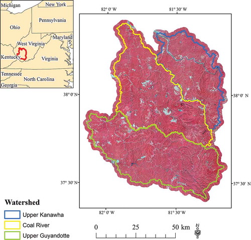
The study area was defined relative to Hydrologic Unit Code (HUC 8) watershed extents within the MTR/VF region of West Virginia, USA (Figure 1). Three adjacent watersheds were mapped: the Upper Kanawha, Upper Guyandotte, and Coal River, totalling 6085 km². These watersheds were selected due to the availability of pre- and post-mining terrain data, digital mine permit extents, and aerial orthophotography. Also, a prior land cover analysis found that within these watersheds surface mining and mine reclamation comprise a major component of the landscape, as much as 6% of the surface area (Maxwell et al. 2011). Watersheds were used to define the study area boundary because watersheds tend to be used as the spatial unit for both management and environmental research.

Figure 1. Location map showing the state of West Virginia and the study area extent. Base imagery is 2011 NAIP orthophotography displayed in false colour (bands 4, 3, and 2 as red, green, and blue). Large cyan patches generally correspond to active mining areas. Surface mining is extensive throughout these watersheds.

4. Methods

4.1. Overview of mapping process

Prior to a detailed description of the methods, we first give a brief overview of the mapping process (Figure 2). The classification is hierarchical, with two stages. First, after preprocessing, the aerial orthophotography was classified using a GEOBIA approach, in which the imagery was segmented and then classified using SVM to produce four classes: woody vegetation, herbaceous vegetation, barren areas, and water. The resulting land cover classification was then generalized using a sieving operation to remove land-cover patches less than 1 ha, the minimum mapping unit (MMU) for the study. Contiguous areas of herbaceous cover (i.e. grasses) were then merged as single objects for the second stage of the classification, in which the RF algorithm along with pre- and post-mining terrain variables were used to differentiate mine-reclaimed grasslands from other grasslands. The results were then assessed using randomized validation data. The following sections elaborate on these methods.

Figure 2. Overview of mapping and assessment process.

4.2. Input data and preprocessing

National Agriculture Imagery Program (NAIP) orthophotography was the primary image data used in this study. The images were collected during the growing season of 2011 between 10 July 2011 and 6 October 2011 with an Intergraph Z/I Imaging Digital Mapping Camera (DMC). The data were provided at a 1 m ground sampling distance (GSD) with four spectral bands (blue, green, red, and near-infrared (NIR)) by the United States Department of Agriculture (USDA) Farm Service Agency. NAIP orthophotography has been used for LULC classification in previous studies (for example, Baker et al. 2013; Davies et al. 2010; Maxwell et al. 2014a). In a previous study (Maxwell et al. 2014a) using NAIP imagery, and focusing only on land cover classes within a single mine in this region, we found that classification accuracies were above 90% when the number of classes was limited and the spatial resolution was decreased from 1 to 5 m. In order to prepare the imagery for segmentation and classification, each uncompressed quarter quadrangle was resampled to a 5 m cell size using pixel aggregation (i.e. average of the input cells) within Erdas Imagine 2014 (ERDAS Imagine 2013). The resampled quarter quadrangles were then mosaicked to produce a single image for the entire study area.

A pre-mining, historic DEM was produced from United States Geologic Survey (USGS) digital line graph (DLG) contour data derived from 1:24,000 topographic maps. These data do not represent a single date; source data range from 1951 to 1989, with the majority of the data representing topographic conditions of the 1960s and 1970s. A review of available terrain data for this region suggested that this is the most appropriate historic elevation data set for this analysis, as pre-mining DEM data are limited. Furthermore, visual inspection of a hillshade image produced from these data and an elevation change image produced by subtracting the historic and recent DEMs both suggest that the DLG data predate almost all large-scale MTR/VF activity in the study area, which began as early as the 1960s but was not widespread until the 1990s (Milici 2000; Wickham et al. 2013). The contour data were gridded on a 9 m raster using the Topo to Raster tool in ArcMap 10.2 (ESRI 2012). A 9 m cell size was chosen, as opposed to a 5 m cell size to match the image data, to reflect the inherent resolution of the DLG data.

A recent, post-mining DEM was made available by the West Virginia Department of Environmental Protection (WVDEP). This DEM was produced using aerial lidar, which is an active remote-sensing technique that uses the two-way travel time of emitted laser pulses and precise geolocation derived from differential global positioning system (GPS) and inertial measurement unit (IMU) data to calculate the elevation of the ground surface and the height of objects above the ground surface (Hyyppä et al. 2009). The lidar data were collected between 9 April 2010 and 29 March 2011 during leaf-off conditions to maximize the number of ground returns. Flight specifications were selected to support a nominal average pulse spacing of 1 m. The Optech ALTM 3100 C sensor was set to a pulse frequency of 70 kHz, a scan frequency of 35 Hz, and a scan angle of 36° (full swath). A 30% overlap was acquired between swaths. The aircraft flew at an average of 1524 m above ground level and at a speed of 125 knots (232 km h⁻¹). The lidar system recorded up to four returns per laser pulse, and each return was classified by the vendor as either ground, non-ground, or as an outlier, and delivered in LAS 1.2 format. The DEM provided by the WVDEP was resampled using pixel aggregation to a 9 m cell size, to match that of the pre-mining DEM.

4.3. Image segmentation and classification

The NAIP orthophotography was segmented using the multi-resolution image segmentation algorithm within eCognition 8.0 (Trimble, Sunnydale, California). This algorithm requires the user to define three parameters: scale, shape, and compactness. The scale parameter controls the size of the image objects (Liu and Xia 2010; Kim et al. 2011), and a number of studies have suggested that this parameter has the largest impact on subsequent classification accuracy (Blaschke 2003; Meinel and Neubert 2004; Kim, Madden, and Warner 2009; Myint et al. 2011). The shape parameter controls the relative importance assigned to the shape of the object versus the ‘colour,’ which relates to spectral properties. Compactness controls the balance between the edge length and form of the object (Baatz and Schäpe 2000). As is common in GEOBIA (e.g. Laliberte, Fredrickson, and Rango 2007; Mathieu, Aryal, and Chong 2007; Dingle Robertson and King 2011; Myint et al. 2011; Duro, Franklin, and Dubé 2012a, 2012b), trial-and-error and expert judgement were used to select the optimal settings of 30 for scale, 0.1 for shape, and 0.5 for compactness. All four image bands were equally weighted in the segmentation. Over 500,000 objects were generated.

The resulting image objects were classified using the implementation of the SVM algorithm available in the e1071 package (Meyer et al. 2012) within the statistical software tool R (R Core Development Team 2012). SVM was chosen because our prior research within this landscape suggested that SVM typically provides more accurate spectral classifications in comparison with RF and boosted classification and regression trees (CART) (Maxwell et al. 2014a, 2014b, 2015). A total of 9409 objects were used to train the algorithm. These objects were selected based on manual interpretation of the 2011 NAIP orthophotography, prior 2007 NAIP orthophotography, mine permit data made available by the WVDEP, and the digital terrain data. For the classification, a RBF kernel was used and the user-defined parameters C and kernel-specific gamma (γ) were optimized using tenfold cross-validation in which the training data were partitioned into 10 unique training sets, using a random assignment, and the classifier was trained 10 times using 90% of the data and withholding the other 10% for validation.

The primary aim of the first stage of the classification was to map grasslands. However, as an intermediate step, the objects were classified as woody vegetation, herbaceous vegetation, barren areas, and water. These classes were chosen based on our prior experience of common land-cover conditions in this landscape (Maxwell et al. 2014a, 2014b, 2015), which suggests these classes are separable given only spectral data. After classification, contiguous areas of land cover smaller than the 1 ha MMU were removed using a sieving operation and replaced with the dominant surrounding class. A 1 ha MMU was selected because reclamation practices in this area commonly result in large patches, typically over 1 ha, of similar land cover. Groups of adjacent objects that were classified as grassland cover were then combined into single objects. The resulting objects were further classified in the next classification stage.

4.4. Differentiation of grasslands

In the second stage of the classification, image objects that were previously labelled as herbaceous vegetation in the initial classification were divided into mine-reclaimed grasslands and non-mining grasslands (Table 1) using the pre- and post-mining terrain characteristics of each object. Although SVM was used for the first stage of the classification discussed above (i.e. the land-cover classification using spectral data), RF was used for the second stage of the analysis, separating the grassland classes, as RF was assumed to be more suitable for modelling the complex interactions between the highly correlated terrain variables (Burkholder et al. 2011). In addition, RF was chosen because it offers measures of variable importance, as well as an estimate of error from the OOB samples.

Table 1. Grassland class definitions.

Land cover class	Description
Non-mining grasslands	Grasslands not resulting from mine reclamation, including pastureland, herbaceous dominated residential development, and other areas on the landscape dominated by herbaceous vegetation.
Mine-reclaimed grasslands	Grasslands resulting from mine reclamation, including reclaimed lands within mine sites and valley fills dominated by herbaceous vegetation.

Predictor variables for the RF classification were derived from the pre- and post-mining DEM data. These variables are summarized in Table 2. Topographic slope (in degrees) was calculated using the Spatial Analyst Extension of ArcMap 10.2 (Burrough and McDonell 1998; ESRI 2012), whereas the other terrain attributes were calculated using the ArcGIS Geomorphometry & Gradient Metrics Toolbox (Evans et al. 2014). The metrics calculated included CTMI (Moore et al. 1993; Gessler et al. 1995), slope position (Berry 2002), roughness (Blaszczynski 1997; Riley, DeGloria, and Elliot 1999), and dissection (Evans 1972). Slope position, roughness, and dissection rely on focal statistics calculated using a moving window; thus, the result is dependent on the window size used. For this study, we used window sizes of 11 pixels × 11 pixels, 21 pixels × 21 pixels, and 31 pixels × 31 pixels (i.e. 99 m × 99 m, 189 m × 189 m, and 279 m × 279 m) and averaged the results. These window sizes were assumed to approximate the hillslope scale, the scale of interest, and were selected by estimating the range of typical valley to ridge distances in this landscape. An elevation change grid was also produced by subtracting the pre-mining DEM from the post-mining DEM. Positive values indicate increases in elevation (e.g. fills) whereas negative values indicate decreased elevation (e.g. excavation).

Table 2. Descriptions of terrain characteristics.

Measure	Description	Reference	Object summary statistics
Elevation (ele)	Elevation Z	NA	Mean, min, max, std
Slope (°) (slp)	Slope (gradient or rate of maximum change in Z)	Burrough and McDonell (1998)	Mean, min, max, std
	atan × 57.29578
Compound topographic moisture index (CTMI)	Measure of steady state wetness as estimated from terrain characteristics	Gessler et al. (1995)Moore et al. (1993)	Mean
	)
Slope position	Scalable slope position	Berry (2002)	Mean
	Z − Zmean
Roughness	Roughness or terrain complexity index	Riley, DeGloria, and Elliot (1999) Blaszczynski (1997)	Mean
Dissection	Dissection of landscape index	Evans (1972)	Mean
Elevation change (ele change)	Pre-Mining Elevation – Post-Mining Elevation	Not applicable	Mean, min, max, std
	Zpost-mining − Zpre-mining

Within each image object, summary mean, minimum, maximum, and standard deviation were calculated for pre- and post-mining elevation and slope, and also elevation change. For all other variables, only the mean was calculated (Table 2). Classifications were produced using the DEM-derived input variable combinations described in Table 3. As a baseline for the comparisons, a classification was also performed using only the spectral data derived from the NAIP imagery as band means and standard deviations (eight predictor variables) for each grassland object.

Table 3. Input variable combinations compared.

Classification	Variables used in the classification	Number of variables
1	All pre- and post-mining DEM-derived variables plus elevation change summary variables	28
2	All pre- and post-mining DEM-derived variables (but excluding elevation change)	24
3	Pre- and post-mining elevation and slope plus elevation change summary variables	20
4	Pre- and post-mining elevation and slope summary variables	16
5	All pre-mining DEM-derived summary variables	12
6	All post-mining DEM-derived summary variables	12
7	Pre-mining elevation and slope summary variables	8
8	Post-mining elevation and slope summary variables	8
9	Elevation change summary variables	4
10	Spectral data (band means and standard deviations)	8

A total of 200 randomly chosen objects were used to train the model, 100 from each of the grassland classes. The RF algorithm from the randomForest package (Liaw and Wiener 2002) within the statistical software tool R (R Core Development Team 2012) was used. A total of 500 trees were used in the ensemble, as this was found to be adequate to produce a stable classification result. The number of variables randomly sampled as candidates at each node (m) was optimized for each input variable combination using tenfold cross-validation.

4.5. Classification assessment

The primary data set used in the classification assessment was selected using simple random sampling across the entire study area of the three watersheds. Samples were collected from three classes: mine-reclaimed grasslands, non-mining grasslands, and non-grass cover. Because grassland cover makes up a relatively small proportion of the study site, random sampling will of course likely produce a relatively small proportion of grassland samples in the validation data set. One possible way to address this imbalance is to employ stratified random sampling, equalized by class. However, since this study involved comparisons of the accuracies of multiple maps, we chose not to use stratification because that approach causes additional complexity in the subsequent calculation of statistics for all the maps, except the specific one used to provide the strata. Although Stehman (2014) provides a straightforward way to calculate this correction for the estimation of population error matrices, it is not clear how to account for this in other statistics, for example, the McNemar’s test, discussed below. Consequently, we chose instead to generate a very large sample, 3000 points, so that grassland classes, despite covering a small extent, would still produce around 100 points for each class, thus ensuring a sufficient sample size for generating the user’s and producer’s accuracies.

The random points were validated using visual interpretation of a variety of layers including 2011 NAIP orthophotography, 2007 NAIP orthophotography, pre-mining slope data, post-mining slope data, a pre-mining hillshade image, a post-mining hillshade image, the elevation change raster grid, and WVDEP surface mine permit data. Five of the 3000 points were removed from the analysis as the correct class was uncertain due to change in land cover between the dates of the NAIP orthophotography and post-mining terrain data collection (i.e. the lidar data).

A variety of methods were used to assess the classifications including the following: traditional accuracy assessment using randomized validation data and error matrices, OOB estimates of generalization error and variable importance provided by RF, and an assessment of confusion between mine-reclaimed grasslands and non-mining grasslands using a randomized sample within areas classified as herbaceous vegetation. These methods will be discussed in more detail below.

One strength of the RF algorithm is its ability to estimate classification error using the withheld, or OOB, data (Breiman 2001; Rodríguez-Galiano et al. 2012a, 2012b). Lawrence, Wood, and Sheley (2006) and Rodríguez-Galiano et al. (2012b) suggest that this accuracy assessment is reliable and unbiased when randomized validation data are used, as in this study. As a result, this estimate of classification accuracy was used to assess the accuracy of separating mine-reclaimed grasslands from other grasslands, the second stage of the classification. The algorithm also generates a measure of variable importance during the training process by excluding each variable sequentially and recording the resulting OOB error (Breiman 2001; Rodríguez-Galiano et al. 2012a, 2012b). This ancillary output of RF was used to assess the contribution of specific terrain measures calculated for the grassland objects (e.g. pre-mining mean elevation, post-mining mean elevation, mean elevation change, pre-mining mean slope position, post-mining mean terrain roughness, etc.).

In order to evaluate the statistical significance of any differences in the classifications, the results were compared on a pairwise basis using McNemar’s test (Dietterich 1998; Foody 2004). McNemar’s test is a test of statistical difference that generates a z-score under the null hypothesis that the classifications are not different. A z-score larger than 1.645 indicates a 95% confidence of statistical significance for the one-directional test of whether one classification is more accurate than the other (Bradley 1968; Dietterich 1998; Foody 2004; Agresti 2007). This statistical test was used to assess the statistical difference between the classifications. It was also used to assess the separability or differentiation of mine-reclaimed grasslands and other grasslands (i.e. the second stage of the classification), using a second set of 1000 random validation points from within areas mapped as grasslands. Of the 1000 original sample points, 33 were removed from the analysis as they could not be interpreted due to landscape change between the dates of the 2011 NAIP orthophotography and post-mining terrain data collection, or because they were interpreted as not being grasslands (i.e. were incorrectly mapped as grasslands).

5. Results and discussion

5.1. Classification accuracy

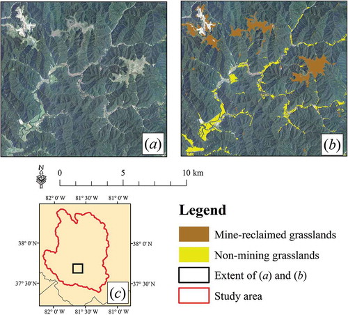
Using different terrain input variable combinations, the overall accuracy of the classifications ranged from 97.4% to 97.9% (Table 4). Overall, the most accurate classifications generally used a combination of pre- and post-mining terrain variables or variables derived from the pre-mining surface only. Figure 3 shows the grassland classification for the entire study area produced using all pre-and post-mining terrain variables plus elevation change variables in the second stage of the classification. Figure 4 shows an example of the same result in greater detail, but for a smaller area and overlaid on the NAIP imagery. Table 5 summarizes the confusion matrix for this classification.

Table 4. Summary statistics for classification of three classes (not grassland, non-mining grasslands, mine-reclaimed grasslands).

			Mine-reclaimed grasslands		Non-mining grasslands		Not grassland
Variables used	Data set	OA (%)	UA (%)	PA (%)	UA (%)	PA (%)	UA (%)	PA (%)
All pre-/post-mining + ele change	1	97.9	89	81	82	72	99	99
All pre-/post-mining	2	97.9	88	80	81	72	99	99
Pre-/post-mining ele and slp + ele change	3	97.9	86	83	85	69	99	99
Pre-/post-mining ele and slp	4	97.7	83	78	80	67	99	99
All pre-mining	5	97.9	88	79	80	72	99	99
All post-mining	6	97.6	82	77	78	65	99	99
Pre-mining ele and slp	7	97.8	87	79	79	70	99	99
Post-mining ele and slp	8	97.4	77	77	76	57	99	99
Ele change	9	97.9	86	83	84	69	99	99
Spectral data (no terrain data)	10	97.2	78	72	66	57	99	99

Notes: The optimal value in each column is shaded grey. OA, overall accuracy; UA, user’s accuracy; PA, producer’s accuracy.

Table 5. Error matrix for classification using all predictor variables (All pre- and post-mining variables plus elevation change in the second stage of the classification).

		Reference data
		Not grassland	Non-mining grasslands	Mine-reclaimed grasslands	Total	User’s accuracy (%)
Classified data	Not grasslands	2780	18	19	2817	99
	Non-mining grasslands	10	60	3	73	82
	Mine-reclaimed grasslands	7	5	93	105	89
	Total	2797	83	115
	Producer’s accuracy (%)	99	72	81

Note: Overall accuracy is 97.9% for separating the three classes.

Figure 3. Grassland classification for entire study area using all predictor variables (all pre- and post-mining variables plus elevation change in the second stage of the classification).

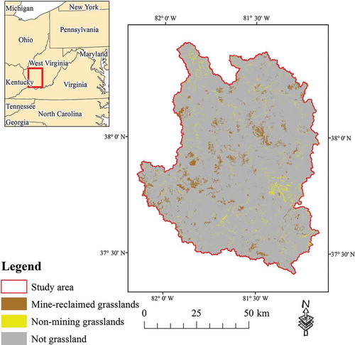
Figure 4. (a) NAIP simulated natural colour image (bands 3, 2, 1 as red, green, and blue). (b) NAIP image with example grassland classification using all predictor variables (all pre- and post-mining variables plus elevation change in the second stage of the classification). (c) Location map.

For the various combinations of terrain data, user’s accuracy for mine-reclaimed grasslands ranged from 77% to 89% and producer’s accuracy from 77% to 83% (Table 4). For non-mining grasslands user’s accuracy ranged from 76% to 85% and producer’s accuracy from 57% to 72%. The lower producer’s accuracy for non-mining grasslands is due to confusion with both mine-reclaimed grasslands and non-grassland cover. Non-grassland cover was generally differentiated from grassland cover with user’s and producer’s accuracies above 98%.

Overall, these data suggest that grasslands can be accurately differentiated from other land-cover types using GEOBIA, SVM, and NAIP orthophotography. In addition, the results indicate that terrain variables are useful for differentiating non-mining and mine-reclaimed grasslands, as using only spectral data in the second stage of the classification yielded the lowest overall accuracy (97.2%), and, most importantly, the lowest user’s and producer’s accuracies for both grassland classes (57–78%). This result is not particularly surprising, since we expected mine-reclaimed grasslands to be very similar spectrally to non-mining grasslands.

Because grasslands are only a small part of the overall landscape, the difference in overall accuracy between the classifications with different topographical variables varied by only 0.4%. However, the user’s and producer’s accuracies for the two grassland categories varied widely, and consequently the classifications were statistically different for many of the combinations, as shown by McNemar’s test (Table 6). This confirms that the choice of input terrain predictor variables affects the accuracy of the classification. Furthermore, all classifications that used terrain variables, with the exception of the combination utilizing only post-mining terrain summary statistics for elevation and slope, were statistically more accurate than the classification using spectral data.

Table 6. McNemar’s test results for classification of three classes (not grassland, non-mining grasslands, mine-reclaimed grasslands).

	Data set	1	2	3	4	5	6	7	8	9
All pre-/post-mining + ele change	1
All pre-/post-mining	2	0.447
Pre-/post-mining ele and slp + ele change	3	0.000	0.333
Pre-/post-mining ele and slp	4	2.111*	1.897*	2.111*
All pre-mining	5	0.817	1.000	0.632	1.508
All post-mining	6	2.673*	2.324*	2.673*	0.655	2.000*
Pre-mining ele and slp	7	1.414	1.134	1.265	1.000	0.707	1.414
Post-mining ele and slp	8	3.400*	3.138*	3.710*	2.041*	2.887*	1.698*	2.837*
Ele change	9	0.333	0.000	0.447	1.500	0.258	2.065*	0.832	3.138*
Spectral data (no terrain data)	10	3.888*	3.667*	4.131*	2.744*	3.452*	1.982*	3.212*	0.949	4.017*

Note: A z-score larger than 1.645 (*) indicates a 95% confidence interval of statistical significance for the one-directional test of whether one classification is more accurate than the other.

5.2. Importance of pre- and post-mining terrain data for differentiating mine-reclaimed and non-mining grasslands

The discussion so far has focused on statistics generated from the entire classification map. In order to explore the second stage of the classification more closely, we now focus exclusively on the differentiation of mine-reclaimed grasslands and non-mining grassland.

Figure 5 shows OOB error rates for the separation of non-mining and mine-reclaimed grasslands using different input variable combinations. The differentiation error rates using various combinations of terrain variables, as estimated using the OOB data, range from 4.5% (using all pre- and post-mining terrain variables but not elevation change variables) to 16.0% (using only post-mining descriptive statistics for elevation and slope). The error rate using only spectral data in the second stage of the classification was 19.0%, the highest error rate obtained.

Figure 5. OOB error rate estimated by RF algorithm for different input variable combinations.

Using the random samples within the grassland classes, Table 7 shows the McNemar’s test results for assessing the differentiation of mine-reclaimed and non-mining grasslands. Statistical significance was observed between the majority of the input variable combinations, with the spectral data and the post-mining elevation and slope classifications being significantly different (i.e. having a lower accuracy) than all other classifications. The McNemar’s test also confirms that a classification using pre- and post-mining terrain data (i.e. not including statistics derived from elevation change) provided a statistically more accurate differentiation of the two classes than a classification using only post-mining data (z-score = 2.635), but not in comparison with a classification using pre-mining data (z-score = 0.333). Pre-mining data only also produced a statistically more accurate differentiation than post-mining data only (z-score = 2.457).

Table 7. McNemar’s test results for differentiation of non-mining and mine-reclaimed grasslands.

	Data set	1	2	3	4	5	6	7	8	9
All pre-/post-mining + ele change	1
All pre-/post-mining	2	1.604
Pre-/post-mining ele and slp + ele change	3	0.200	1.238
Pre-/post-mining ele and slp	4	2.491*	1.270	2.333*
All pre-mining	5	1.692*	0.333	1.309	1.116
All post-mining	6	4.281*	2.635*	3.878*	1.497	2.457*
Pre-mining ele and slp	7	5.128*	4.621*	4.587*	2.994*	4.619*	0.539
Post-mining ele and slp	8	8.433*	7.209*	8.275*	6.683*	7.030*	6.359*	5.031*
Ele change	9	1.134	0.277	1.180	1.192	0.368	2.652*	3.133*	6.982*
Spectral data (no terrain data)	10	7.898*	6.548*	7.929*	5.933*	6.438*	4.820*	4.353*	0.254	7.233*

Note: A z-score larger than 1.645 (*) indicates a 95% confidence interval of statistical significance for the one-directional test of whether one classification is more accurate than the other.

In summary, these data suggest that mine-reclaimed grasslands have a unique topographic signature compared with other grasslands in this terrain, and can thus be separated from other grasslands using terrain characteristics extracted from DEM data. This is especially true when both pre- and post-mining characteristics are used or when just pre-mining characteristics are used. We attribute the usefulness of pre-mining data to the nature of the terrain alteration resulting from MTR/VF mining. A pre-mining topography characterized by steep slopes and an upper slope position may be more predictive than post-mining terrain characteristics, in which the landscape has been flattened and therefore has become more similar topographically to non-mining grasslands.

5.3. Importance of terrain attributes for differentiating mine-reclaimed and non-mining grasslands

The McNemar’s test (Table 7) comparing the grassland differentiation using all pre- and post-mining predictor variables with and without including the elevation change data yielded a z-score of 1.604. This suggests that the incorporation of descriptive statistics derived from the elevation change surface did not statistically improve the classification accuracy. However, a classification using just the elevation change data was not statistically different from a classification using all of the pre- and post-mining predictor variables excluding elevation change variables (z-score = 0.277). A combination of summary statistics for elevation change and pre- and post-mining elevation and slope was statistically more accurate than a classification using just pre- and post-mining elevation and slope variables (z-score = 2.333). As shown in Figure 6, measures derived from the elevation change surface were of particular importance in the model as estimated by the OOB mean decrease in accuracy measure. These data suggest that there is merit in including elevation change variables, especially when the number of terrain variables used to characterize the pre- and post-mining terrain are limited.

Figure 6. Variable importance as estimated by OOB mean decrease in accuracy for model using all pre- and post-mining elevation (ele), slope (slp), and elevation change (ele change) descriptive statistics.

The incorporation of pre- and post-mining CTMI, slope position, roughness, and dissection in the classification was also assessed. These topographic variables statistically improved the differentiation of the two grassland classes in comparison with using only measures derived from elevation and slope when only post-mining terrain data were used (z-score = 6.359) and when only pre-mining data were used (z-score = 4.619); however, no statistical difference was observed when using a combination of pre- and post-mining data (z-score = 1.270). Figure 7 shows variable importance for the post-mining model as estimated from the OOB mean decrease in accuracy. These data suggest that the additional post-mining terrain variables, beyond elevation and slope, contribute to the model, especially dissection. Figure 8 shows variable importance for the pre-mining model. These data suggest that the added pre-mining variables, beyond elevation and slope, contribute to the model, especially dissection and roughness. However, the most important variable appears to be the pre-mining mean slope. The reason for this is likely because pre-mining slopes of MTR/VF sites are often steep, and thus pre-mining slopes differentiate mine-reclaimed grasslands from non-mining grasslands, which are often found on flatter surfaces (e.g. valley bottoms) in this landscape. These data tend to suggest that derived topographic variables are of value, especially when only pre- or post-mining terrain data are available.

Figure 7. Variable importance as estimated by OOB mean decrease in accuracy for model using all post-mining variables.

Figure 8. Variable importance as estimated by OOB mean decrease in accuracy for model using all pre-mining variables.

5.4. Practical considerations

Pre- and post-mining terrain data were found to be of value for differentiating spectrally similar non-mining and mine-reclaimed grasslands in this study area in West Virginia. However, some practical limitations are present. First, the pre-mining terrain data were of greater importance for differentiating the cover types than post-mining data. The availability of older DEM data for characterizing the pre-mining terrain is generally limited, and in this study it was necessary to produce a DEM from the available DLG data as a historical DEM was not readily available. Further, USGS DLG contour data were collected over a wide range of dates and were derived from photogrammetric methods, making comparison to the recent lidar-derived data complex (DeWitt, Warner, and Conley 2015). In addition, the DLG data may not predate all mining. Second, post-mining terrain data may not be temporally coincident with the available imagery. For example, in this study, the NAIP orthophotography was collected over a period of nearly three months, and the lidar data were collected over a period of nearly two years. Planning temporally coincident collections of high-resolution imagery and lidar may be difficult, especially over large spatial extents. For studies with limited budgets that must exploit data originally collected for other purposes, as in this study, the challenges of finding data of similar dates are even greater.

Many of the terrain attributes calculated rely on focal statistics calculated using a moving window. Selecting the appropriate window size can be difficult as the optimal window size may be case-specific and guidance from the literature on the appropriate scale is limited. This presents a challenge when working with DEM-derived terrain attributes for LULC classification.

Despite these limitations, our results suggest that multi-temporal terrain data summarized for image objects offers a means to differentiate spectrally similar LULC classes that have a characteristic topographic signature. This is especially true when machine learning algorithms are used to classify such data. Such methods may be appropriate for augmenting available data sets to support a specific modelling or analysis task, such as the National Land Cover Dataset (NLCD).

6. Conclusions

This research investigated the use of multi-temporal terrain data for differentiating these topographically distinctive features. Surface mining produces extensive landscape alterations that persist as a legacy of LULC alteration. Mine-reclaimed land cover has been shown to have important impacts on hydrology, terrestrial habitats, and aquatic ecosystems. Thus, it is of importance to differentiate such grasslands from other grasslands on the landscape.

The classification approach employed, which makes use of GEOBIA, machine learning algorithms, high-resolution aerial imagery, and multi-temporal terrain characteristics derived from DEMs, provided an accurate means to differentiate grassland cover from other land cover.

Mine-reclaimed grasslands were mapped with user’s and producer’s accuracies between 77% and 89% using multi-temporal terrain data. Classifications using either a combination of pre- and post-mining terrain variables or only pre-mining terrain variables generally outperformed classifications using only post-mining terrain data. Elevation change data were of value, and terrain characteristics as CTMI, slope position, roughness, and dissection generally improved the classification.

GEOBIA was proven to be a valuable tool for combining data collected using different sensors and gridded at variable cell sizes (i.e. the image and digital terrain data). In addition, GEOBIA provided a mechanism to characterize the terrain data using summary variables (e.g. mean, maximum, minimum, standard deviation, etc.) at the object scale. Differentiating landscape position from attributes derived from DEMs is not straightforward because the scale of the landscape is complex, with multiple potential topographic scales present. Also, a single site might include more than one topographic class. With GEOBIA, by integrating over an object, these problems can potentially be overcome.

The machine learning algorithms were particularly useful in incorporating the ancillary data derived from the DEMs, since these most likely would not have met the basic assumptions of multivariate normality required for parametric classifiers. In addition, the RF classifier was particularly useful due to its ability to provide estimates of accuracy and also variable importance.

This study highlights the importance of maintaining legacy elevation products (e.g. DLG) with descriptive metadata regarding year of acquisition or creation, since the pre-mining terrain data were shown to be of great value in this study. We know of no formal effort to archive historical elevation data sets analogous to the extensive image archives that are maintained by the USGS, the National Aeronautic and Space Administration (NASA), and other government agencies. We recommend that developing such archives should be a priority.

Disclosure statement

No potential conflict of interest was reported by the authors.

Acknowledgements

Lidar data were provided by the West Virginia Department of Environmental Protection (WVDEP) and the Natural Resource Analysis Center (NRAC) at West Virginia University. We would specifically like to acknowledge Adam Riley and Paul Kinder for their assistance in obtaining and processing the lidar data. We would like to thank two anonymous reviewers for their helpful comments that greatly improved the manuscript.

Additional information

Funding

Funding support for this study was provided by West Virginia View and the Appalachian College Association. The project described in this publication was also supported in part by grant number G14AP00002 from the Department of the Interior, United States Geological Survey to AmericaView. Its contents are solely the responsibility of the authors; the views and conclusions contained in this document are those of the authors and should not be interpreted as representing the opinions or policies of the US Government. Mention of trade names or commercial products does not constitute their endorsement by the US Government.

References

- Agresti, A. 2007. An Introduction to Categorical Data Analysis. Vol. 400. 2nd ed. Hoboken, NJ: Wiley-Interscience.
- Anderson, A. T., D. Schultz, N. Buchman, and H. M. Nock. 1997. “Landsat Imagery for Surface-Mine Inventory.” Photogrammetric Engineering and Remote Sensing 43 (8): 1027–1036.
- Anderson, J. R., E. E. Hardy, J. T. Roach, and R. E. Witmer. 1976. A Land-Use and Land Cover Classification System for Use with Remote Sensor Data. Geologic Survey Professional Paper No. 964. Washington, DC: US Government Printing Office.
- Baatz, M., and A. Schäpe. 2000. “Multiresolution Segmentation – An Optimization Approach for High Quality Multi-Scale Image Segmentation.” In Angewandte Geographische Informationsverarveitung XII, edited by J. Strobl, T. Blaschke, and G. Griesebener, 12–23. Berlin: Herbert Wichmann Verlag.
- Baker, B. A., T. A. Warner, J. F. Conley, and B. E. McNeil. 2013. “Does Spatial Resolution Matter? A Multi-Scale Comparison of Object-Based and Pixel-Based Methods for Detecting Change Associated with Gas Well Drilling Operations.” International Journal of Remote Sensing 34 (5): 1633–1651. doi:10.1080/01431161.2012.724540.
- Bernhardt, E. S., B. D. Lutz, R. S. King, J. P. Fay, C. E. Carter, A. M. Helton, D. Campagna, and J. Amos. 2012. “How Many Mountains Can We Mine? Assessing the Regional Degradation of Central Appalachian Rivers by Surface Coal Mining.” Environmental Science and Technology 46 (15): 8115–8122. doi:10.1021/es301144q.
- Bernhardt, E. S., and M. A. Palmer. 2011. “The Environmental Costs of Mountaintop Mining Valley Fill Operations for Aquatic Ecosystems of the Central Appalachians.” Annals of the New York Academy of Sciences 1223 (1): 39–57. doi:10.1111/j.1749-6632.2011.05986.x.
- Berry, J. K. 2002. “Beyond Mapping Use Surface Area for Realistic Calculations.” Geo World 15 (9): 20–21.
- Blaschke, T. 2003. “Object-Based Contextual Image Classification Built on Image Segmentation.” 2003 IEEE Workshop on Advances in Techniques for Analysis of Remotely Sensed Data, Greenbelt, MD, October 27–28, 13–119.
- Blaschke, T. 2010. “Object Based Image Analysis for Remote Sensing.” ISPRS Journal of Photogrammetry and Remote Sensing 65 (1): 2–16. doi:10.1016/j.isprsjprs.2009.06.004.
- Blaschke, T., G. J. Hay, M. Kelly, S. Lang, P. Hofmann, E. Addink, R. Q. Feitosa, F. Van Der Meer, H. Van Der Werff, F. Van Coillie, and D. Tiede. 2014. “Geographic Object-Based Image Analysis – Towards a New Paradigm.” ISPRS Journal of Photogrammetry and Remote Sensing 87 (100): 180–191. doi:10.1016/j.isprsjprs.2013.09.014.
- Blaschke, T., and J. Strobl. 2001. “What’s Wrong with Pixels? Some Recent Developments Interfacing Remote Sensing and GIS.” GIS – Zeitschrift Für Geoinformationssysteme 14 (6): 12–17.
- Blaszczynski, J. S. 1997. “Landform Characterization with Geographic Information Systems.” Photogrammetric Engineering and Remote Sensing 63 (2): 183–191.
- Bradley, J. V. 1968. Distribution-Free Statistical Tests. Vol. 388. Englewood Cliffs, NJ: Prentice Hall.
- Breiman, L. 1996. “Bagging Predictors.” Machine Learning 24 (2): 123–140. doi:10.1007/BF00058655.
- Breiman, L. 2001. “Random Forests.” Machine Learning 45 (1): 5–32. doi:10.1023/A:1010933404324.
- Burges, C. J. C. 1998. “A Tutorial on Support Vector Machines for Pattern Recognition.” Data Mining and Knowledge Discovery 2 (2): 121–167. doi:10.1023/A:1009715923555.
- Burkholder, A., T. A. Warner, M. Culp, and R. E. Landenberger. 2011. “Seasonal Trends in Separability of Leaf Reflectance Spectra for Ailanthus Altissima and Four Other Tree Species.” Photogrammetric Engineering and Remote Sensing 77 (8): 793–804. doi:10.14358/PERS.77.8.793.
- Burrough, P. A., and R. A. McDonell. 1998. Principles of Geographical Information Systems. Vol. 356. 2nd ed. New York: Oxford University Press.
- Chubey, M. S., S. E. Franklin, and M. A. Wulder. 2006. “Object-Based Analysis of IKONOS-2 Imagery for Extraction of Forest Inventory Parameters.” Photogrammetric Engineering and Remote Sensing 72 (4): 383–394. doi:10.14358/PERS.72.4.383.
- Cihlar, J., and L. J. M. Jansen. 2001. “From Land Cover to Land Use: A Methodology for Efficient Land Use Mapping Over Large Areas.” The Professional Geographer 53 (2): 275–289. doi:10.1080/00330124.2001.9628460.
- Cutler, D. R., T. C. Edwards Jr., K. H. Beard, A. Cutler, K. T. Hess, J. Gibson, and J. J. Lawler. 2007. “Random Forests for Classification in Ecology.” Ecology 88 (11): 2783–2792. doi:10.1890/07-0539.1.
- Davies, K. W., S. L. Petersen, D. D. Johnson, D. B. Davis, M. D. Madsen, D. L. Zvirzdin, and J. D. Bates. 2010. “Estimating Juniper Cover from National Agriculture Imagery Program (NAIP) Imagery and Evaluating Relationships between Potential Cover and Environmental Variables.” Rangeland Ecology and Management 63 (6): 630–637. doi:10.2111/REM-D-09-00129.1.
- DeWitt, J. D., T. A. Warner, and J. F. Conley. 2015. “Comparison of DEMS Derived from USGS DLG, SRTM, a Statewide Photogrammetry Program, ASTER GDEM and Lidar: Implications for Change Detection.” GIScience and Remote Sensing 52 (2): 179–197. doi:10.1080/15481603.2015.1019708.
- Dietterich, T. G. 1998. “Approximate Statistical Tests for Comparing Supervised Classification Learning Algorithms.” Neural Computation 10 (7): 1895–1923. doi:10.1162/089976698300017197.
- Dingle Robertson, L., and D. J. King. 2011. “Comparison of Pixel- and Object-Based Classification in Land Cover Change Mapping.” International Journal of Remote Sensing 32 (6): 1505–1529. doi:10.1080/01431160903571791.
- Drăguţ, L., and T. Blaschke. 2006. “Automated Classification of Landform Elements Using Object-Based Image Analysis.” Geomorphology 81 (3–4): 330–344. doi:10.1016/j.geomorph.2006.04.013.
- Duro, D. C., S. E. Franklin, and M. G. Dubé. 2012a. “A Comparison of Pixel-Based and Object-Based Image Analysis with Selected Machine Learning Algorithms for the Classification of Agricultural Landscapes using SPOT-5 HRG Imagery.” Remote Sensing of Environment 118: 259–272. doi:10.1016/j.rse.2011.11.020.
- Duro, D. C., S. E. Franklin, and M. G. Dubé. 2012b. “Multi-Scale Object-Based Image Analysis and Feature Selection of Multi-Sensor Earth Observation Imagery Using Random Forests.” International Journal of Remote Sensing 33 (14): 4502–4526. doi:10.1080/01431161.2011.649864.
- Ehlke, T. A., G. S. Runner, and S. C. Downs. 1982. “Hydrology of Area 9, Eastern Coal Province, West Virginia.” United States Geological Survey Water-Resources Investigation. Vol. 63. Open File Report 81-803.
- ERDAS Imagine. 2013. ERDAS Field Guide. Vol. 792. Huntsville, AL: Intergraph Corporation.
- ESRI. 2012. ArcGIS Desktop: Release 10.1. Redlands, CA: Environmental Systems Research Institute.
- Evans, I. S. 1972. “General Geomorphometry, Derivatives of Altitude, and Descriptive Statistics.” In Spatial Analysis in Geomorphology, edited by R. J. Chorley, 17–90. New York: Harper & Row.
- Evans, J. S., and J. M. Kiesecker. 2014. “Shale Gas, Wind and Water: Assessing the Potential Cumulative Impact of Energy Development on Ecosystem Services within the Marcellus Play.” Plos One 9 (2): e89210. doi:10.1371/journal.pone.0089210.
- Evans, J. S., J. Oakleaf, S. A. Cushman, and D. Theobald. 2014. “An ArcGIS Toolbox for Surface Gradient and Geomorphometric Modeling. Version 2.0-0.” Accessed March 122015. http://evansmurphy.wix.com/evansspatial
- Ferrari, J. R., T. R. Lookingbill, B. McCormick, P. A. Townsend, and K. N. Eshleman. 2009. “Surface Mining and Reclamation Effects on Flood Response of Watersheds in the Central Appalachian Plateau Region.” Water Resources Research 45 (4): 1–11. doi:10.1029/2008WR007109.
- Folke, C., L. Pritchard, Jr., F. Berkes, J. Colding, and U. Svedin. 2007. “The Problem of Fit between Ecosystems and Institutions: Ten Years Later.” Ecology and Society 12 (1): 30.
- Foody, G. M. 2004. “Thematic Map Comparison: Evaluating the Statistical Significance of Differences in Classification Accuracy.” Photogrammetric Engineering and Remote Sensing 70 (5): 627–633. doi:10.14358/PERS.70.5.627.
- Fritz, K. M., S. Fulton, B. R. Johnson, C. D. Barton, J. D. Jack, D. A. Word, and R. A. Burke. 2010. “Structural and Functional Characteristics of Natural and Constructed Channels Draining a Reclaimed Mountaintop Removal and Valley Fill Coal Mine.” Journal of the North American Benthological Society 29 (2): 673–689. doi:10.1899/09-060.1.
- Gessler, P. E., I. D. Moore, N. J. McKenzie, and P. J. Ryan. 1995. “Soil-Landscape Modelling and Spatial Prediction of Soil Attributes.” International Journal of GIS 9 (4): 421–432.
- Gislason, P. O., J. A. Benediktsson, and J. R. Sveinsson. 2006. “Random Forests for Land Cover Classification.” Pattern Recognition Letters 27 (4): 294–300. doi:10.1016/j.patrec.2005.08.011.
- Hansen, M. C., and B. Reed. 2000. “A Comparison of the IGBP DISCover and University of Maryland 1 km Global Land Cover Products.” International Journal of Remote Sensing 21 (6–7): 1365–1373. doi:10.1080/014311600210218.
- Hartman, K. J., M. D. Kaller, J. W. Howell, and J. A. Sweka. 2005. “How Much Do Valley Fills Influence Headwater Streams?” Hydrobiologia 532: 91–102. doi:10.1007/s10750-004-9019-1.
- Hooke, R. L. 1994. “On the Efficacy of Humans as Geomorphic Agents.” GSA Today 4 (9): 217, 224–225.
- Hooke, R. L. 1999. “Spatial Distribution of Human Geomorphic Activity in the United States: Comparison to Rivers.” Earth Surface Processes and Landforms 24 (8): 687–692.
- Hyyppä, J., W. Wagner, M. Hollaus, and H. Hyyppä. 2009. “Airborne Laser Scanning.” In The SAGE Handbook of Remote Sensing, edited by T. A. Warner, M. D. Nellis, and G. M. Foody, 199–212. London: Sage Publications.
- Irons, J. R., and R. L. Kennard. 1986. “The Utility of Thematic Mapper Sensor Characteristics for Surface Mine Monitoring.” Photogrammetric Engineering and Remote Sensing 52: 389–396.
- Joachims, T. 1998. “Text Categorization with Support Vector Machines: Learning with Many Relevant Features.” Proceedings of European Conference on Machine Learning, Chemnitz, April 21–23, 137–142.
- Kazar, S. A., and T. A. Warner. 2013. “Assessment of Carbon Storage and Biomass on Minelands Reclaimed to Grassland Environments Using Landsat Spectral Indices.” Journal of Applied Remote Sensing 7 (1): 073583. doi:10.1117/1.JRS.7.073583.
- Ke, Y., L. J. Quackenbush, and J. Im. 2010. “Synergistic Use of Quickbird Multispectral Imagery and LiDAR Data for Object-Based Forest Species Classification.” Remote Sensing of Environment 114: 1141–1154. doi:10.1016/j.rse.2010.01.002.
- Kim, M., M. Madden, and T. A. Warner. 2009. “Forest Type Mapping Using Object-Specific Texture Measures from Multispectral Ikonos Imagery: Segmentation Quality and Image Classification Issues.” Photogrammetric Engineering and Remote Sensing 75 (7): 819–829. doi:10.14358/PERS.75.7.819.
- Kim, M., T. A. Warner, M. Madden, and D. S. Atkinson. 2011. “Multi-Scale GEOBIA with Very High Spatial Resolution Digital Aerial Imagery: Scale, Texture, and Image Objects.” International Journal of Remote Sensing 32 (10): 2825–2850. doi:10.1080/01431161003745608.
- Knight, J. F., B. P. Tolcser, J. M. Corcoran, and L. P. Rampi. 2013. “The Effects of Data Selection and Thematic Detail on the Accuracy of High Spatial Resolution Wetland Classifications.” Photogrammetric Engineering and Remote Sensing 79 (7): 613–623. doi:10.14358/PERS.79.7.613.
- Laliberte, A. S., E. L. Fredrickson, and A. Rango. 2007. “Combining Decision Trees with Hierarchical Object-Oriented Image Analysis for Mapping Arid Rangelands.” Photogrammetric Engineering and Remote Sensing 73 (2): 197–207. doi:10.14358/PERS.73.2.197.
- Lawrence, R. L., S. D. Wood, and R. L. Sheley. 2006. “Mapping Invasive Plants Using Hyperspectral Imagery and Breiman Cutler Classifications (randomForest).” Remote Sensing of Environment 100: 356–362. doi:10.1016/j.rse.2005.10.014.
- Liaw, A., and M. Wiener. 2002. “Classification and Regression by randomForest.” R News 2 (3): 18–22.
- Liu, D., and F. Xia. 2010. “Assessing Object-based Classification: Advantages and limitations.” Remote Sensing Letters 1 (4): 187–194.
- Mathieu, R., J. Aryal, and A. K. Chong. 2007. “Object-Based Classification of Ikonos Imagery for Mapping Large-Scale Vegetation Communities in Urban Areas.” Sensors 7 (11): 2860–2880. doi:10.3390/s7112860.
- Maxwell, A. E., and M. P. Strager. 2013. “Assessing Landform Alterations Induced by Mountaintop Mining.” Natural Science 5 (02): 229–237. doi:10.4236/ns.2013.52A034.
- Maxwell, A. E., M. P. Strager, T. A. Warner, N. P. Zégre, and C. B. Yuill. 2014a. “Comparison of NAIP Orthophotography and RapidEye Satellite Imagery for Mapping of Mining and Mine Reclamation.” GIScience and Remote Sensing 51 (3): 301–320. doi:10.1080/15481603.2014.912874.
- Maxwell, A. E., M. P. Strager, C. Yuill, J. T. Petty, E. Merriam, and C. Mazzarella. 2011. “Disturbance Mapping and Landscape Modeling of Mountaintop Mining Using ArcGIS.” Paper presented at the International ESRI User Conference, San Diego, CA, July 11–15.
- Maxwell, A. E., T. A. Warner, M. P. Strager, J. F. Conley, and A. L. Sharp. 2015. “Assessing Machine Learning Algorithms and Image- and LiDAR-Derived Variables for GEOBIA Classification of Mining and Mine Reclamation.” International Journal of Remote Sensing 36 (4): 954–978. doi:10.1080/01431161.2014.1001086.
- Maxwell, A. E., T. A. Warner, M. P. Strager, and M. Pal. 2014b. “Combining RapidEye Satellite Imagery and LiDAR for Mapping of Mining and Mine Reclamation.” Photogrammetric Engineering and Remote Sensing 80 (2): 179–189. doi:10.14358/PERS.80.2.179-189.
- McCormick, B. C., K. N. Eshleman, J. L. Griffith, and P. A. Townsend. 2009. “Detection of Flooding Responses at the River Basin Scale Enhanced by Land Use Change.” Water Resources Research 45 (8): 1–15. doi:10.1029/2008WR007594.
- Meinel, G., and M. Neubert. 2004. “A Comparison of Segmentation Programs for High Resolution Remote Sensing Data.” International Archives of the ISPRS 35: 1097–1105.
- Merriam, E. R., J. T. Petty, G. T. Merovich, J. B. Fulton, and M. P. Strager. 2011. “Additive Effects of Mining and Residential Development on Stream Conditions in a Central Appalachian Watershed.” Journal of the North American Benthological Society 30 (2): 399–418. doi:10.1899/10-079.1.
- Merriam, E. R., J. T. Petty, M. P. Strager, A. E. Maxwell, and P. F. Ziemkiewicz. 2013. “Scenario Analysis Predicts Context-Dependent Stream Response to Landuse Change in a Heavily Mined Central Appalachian Watershed.” Freshwater Science 32 (4): 1246–1259. doi:10.1899/13-003.1.
- Meyer, D., E. Dimitriadou, K. Hornik, A. Weingessel, and F. Leisch. 2012. “E1071: Misc Functions of the Department of Statistics (E1071). R Package Version 1.6-1.” Accessed March 12 2015. http://CRAN.R-project.org/package=e1071
- Milici, R. C. 2000. “Depletion of Appalachian Coal Reserves – How Soon?” International Journal of Coal Geology 44 (3–4): 251–266. doi:10.1016/S0166-5162(00)00013-6.
- Miller, A. J., and N. P. Zégre. 2014. “Mountaintop Removal Mining and Catchment Hydrology.” Water 6 (3): 472–499. doi:10.3390/w6030472.
- Moore, I. D., P. E. Gessler, G. Z. Nielsen, and G. A. Petersen. 1993. “Terrain Attributes: Estimation Methods and Scale Effects.” In Modeling Change in Environmental Systems, edited by A. J. Jakeman, M. B. Beck, and M. McAleer, 189–214. London: Wiley.
- Myint, S. W., P. Gober, A. Brazel, S. Grossman-Clarke, and Q. Weng. 2011. “Per-Pixel vs. Object-Based Classification of Urban Land Cover Extraction using High Spatial Resolution Imagery.” Remote Sensing of Environment 115: 1145–1161. doi:10.1016/j.rse.2010.12.017.
- Negley, T. L., and K. N. Eshleman. 2006. “Comparison of Stormflow Responses of Surface-Mined and Forested Watersheds in the Appalachian Mountains, USA.” Hydrological Processes 20 (16): 3467–3483. doi:10.1002/(ISSN)1099-1085.
- Pal, M. 2005. “Random Forest Classifier for Remote Sensing Classification.” International Journal of Remote Sensing 26 (1): 217–222. doi:10.1080/01431160412331269698.
- Pal, M., and P. M. Mather. 2005. “Support Vector Machines for Classification in Remote Sensing.” International Journal of Remote Sensing 26 (5): 1007–1011. doi:10.1080/01431160512331314083.
- Palmer, M. A., E. S. Bernhardt, W. H. Schlesinger, K. N. Eshleman, E. Fourfoula-Georgiou, M. S. Hendryx, A. D. Lemly, G. E. Likens, O. L. Loucks, M. E. Power, P. S. White, and P. R. Wilcock. 2010. “Mountaintop Mining Consequences.” Science 327: 148–149. doi:10.1126/science.1180543.
- Parks, N. F., G. W. Petersen, and G. M. Baumer. 1987. “High Resolution Remote Sensing of Spatially and Spectrally Complex Coal Surface Mines of Central Pennsylvania: A Comparison Between SPOT, MSS, and Landsat-5 Thematic Mapper.” Photogrammetric Engineering and Remote Sensing 53 (4): 415–420.
- Pino-Mejías, R., M. D. Cubiles-de-la-Vega, M. Anaya-Romero, A. Pascual-Acosta, A. Jordán López, and N. Bellinfante-Crocci. 2010. “Predicting the Potential Habitat of Oaks with Data Mining Models and the R System.” Environmental Modelling and Software 25 (7): 826–836. doi:10.1016/j.envsoft.2010.01.004.
- Pond, G. J. 2010. “Patterns of Ephemeroptera Taxa Loss in Appalachian Headwater Streams (Kentucky, USA).” Hydrobiologia 641: 185–201. doi:10.1007/s10750-009-0081-6.
- Pond, G. J., M. E. Passmore, F. A. Borsuk, L. Reynolds, and C. J. Rose. 2008. “Downstream Effects of Mountaintop Coal Mining: Comparing Biological Conditions Using Family- and Genus-Level Macroinvertebrate Bioassessment Tools.” Journal of the North American Benthological Society 27 (3): 717–737. doi:10.1899/08-015.1.
- Prakash, A., and R. P. Gupta. 1998. “Land-Use Mapping and Change Detection in a Coal Mining Area - a Case Study in the Jharia Coalfield, India.” International Journal of Remote Sensing 19 (3): 391–410. doi:10.1080/014311698216053.
- Prasad, A. M., L. R. Iverson, and A. Liaw. 2006. “Newer Classification and Regression Tree Techniques: Bagging and Random Forests for Ecological Prediction.” Ecosystems 9: 181–199. doi:10.1007/s10021-005-0054-1.
- R Core Development Team. 2012. R: A Language and Environment for Statistical Computing. Vienna: R Foundation for Statistical Computing. Accessed March 12 2015. http://www.R-project.org.
- Rathore, C. S., and R. Wright. 1993. “Monitoring Environmental Impacts of Surface Coal-Mining.” International Journal of Remote Sensing 14 (6): 1021–1042. doi:10.1080/01431169308904394.
- Riley, S. J., S. D. DeGloria, and R. Elliot. 1999. “A Terrain Ruggedness Index That Quantifies Topographic Heterogeneity.” Intermountain Journal of Science 5: 1–4.
- Rodríguez-Galiano, V. F., M. Chica-Olma, F. Abarca-Hernández, P. M. Atkinson, and C. Jeganathan. 2012b. “Random Forest Classification of Mediterranean Land Cover Using Multi-Seasonal Imagery and Multi-Seasonal Texture.” Remote Sensing of Environment 121: 93–107. doi:10.1016/j.rse.2011.12.003.
- Rodríguez-Galiano, V. F., B. Ghimire, J. Rogan, M. Chica-Olmo, and J. P. Rigol-Sanchez. 2012a. “An Assessment of the Effectiveness of a Random Forest Classifier for Land-Cover Classification.” ISPRS Journal of Photogrammetry and Remote Sensing 67: 93–104. doi:10.1016/j.isprsjprs.2011.11.002.
- Sen, S., C. E. Zipper, R. H. Wynne, and P. F. Donovan. 2012. “Identifying Revegetated Mines as Disturbance/Recovery Trajectories Using an Interannual Landsat Chronosequence.” Photogrammetric Engineering and Remote Sensing 78 (3): 223–235. doi:10.14358/PERS.78.3.223.
- Simmons, J. A., W. S. Currie, K. N. Eshleman, K. Kuers, S. Monteleone, T. L. Negley, B. R. Pohlad, and C. L. Thomas. 2008. “Forest to Reclaimed Mine Land Use Change Leads to Altered Ecosystem Structure and Function.” Ecological Applications 18 (1): 104–118. doi:10.1890/07-1117.1.
- Steele, B. M. 2000. “Combining Multiple Classifiers: An Application Using Spatial and Remotely Sensed Information for Land Cover Type Mapping.” Remote Sensing of Environment 74 (3): 545–556. doi:10.1016/S0034-4257(00)00145-0.
- Stehman, S. V. 2014. “Estimating Area and Map Accuracy for Stratified Random Sampling When the Strata Are Different from the Map Classes.” International Journal of Remote Sensing 35 (13): 4923–4939. doi:10.1080/01431161.2014.930207.
- Townsend, P. A., D. P. Helmers, C. C. Kingdon, B. E. McNeil, K. M. De Beurs, and K. N. Eshleman. 2009. “Changes in the Extent of Surface Mining and Reclamation in the Central Appalachians Detected Using a 1976–2006 Landsat Time Series.” Remote Sensing of Environment 113: 62–72. doi:10.1016/j.rse.2008.08.012.
- Treitz, P., and P. Howarth. 2000. “Integrating Spectral, Spatial, and Terrain Variables for Forest Ecosystem Classification.” Photogrammetric Engineering and Remote Sensing 66 (3): 305–318.
- Trimble. 2011. Ecognition Developer 8.64.1 User Guide. Munich: Trimble.
- Tso, B., and P. Mather. 2003. Classification Methods for Remotely Sensed Data. Vol. 352. New York: CRC Press.
- Vapnik, V. N. 1995. The Nature of Statistical Learning Theory. Vol. 188. New York: Springer-Verlag.
- Walter, V. 2004. “Object-Based Classification of Remote Sensing Data for Change Detection.” ISPRS Journal of Photogrammetry and Remote Sensing 58 (3–4): 225–238. doi:10.1016/j.isprsjprs.2003.09.007.
- Warner, T. A., and F. Nerry. 2009. “Does Single Broadband or Multispectral Thermal Data Add Information for Classification of Visible, Near- and Shortwave Infrared Imagery of Urban Areas?” International Journal of Remote Sensing 30 (9): 2155–2171. doi:10.1080/01431160802549286.
- Weakland, C. A., and P. B. Wood. 2005. “Cerulean Warbler (Dendroica cerulea) Microhabitat and Landscape-Level Habitat Characteristics in Southern West Virginia.” The Auk 122 (2): 497–508. doi:10.1642/0004-8038(2005)122[0497:CWDCMA]2.0.CO;2.
- Wickham, J., P. B. Wood, M. C. Nicholson, W. Jenkins, D. Druckenbrod, G. W. Suter, M. P. Strager, C. Mazzarella, W. Galloway, and J. Amos. 2013. “The Overlooked Terrestrial Impacts of Mountaintop Mining.” BioScience 63 (5): 335–348. doi:10.1525/bio.2013.63.5.7.
- Wickham, J. D., K. H. Riitters, T. G. Wade, M. Coan, and C. Homer. 2007. “The Effect of Appalachian Mountaintop Mining on Interior Forest.” Landscape Ecology 22: 179–187. doi:10.1007/s10980-006-9040-z.
- Wood, P. B., S. B. Bosworth, and R. Dettmers. 2006. “Cerulean Warbler Abundance and Occurrence Relative to Large-Scale Edge and Habitat Characteristics.” The Condor 108 (1): 154–165. doi:10.1650/0010-5422(2006)108[0154:CWAAOR]2.0.CO;2.
- Wright, C., and A. Gallant. 2007. “Improved Wetland Remote Sensing in Yellowstone National Park Using Classification Trees to Combine TM Imagery and Ancillary Environmental Data.” Remote Sensing of Environment 107 (4): 582–605. doi:10.1016/j.rse.2006.10.019.
- Zégre, N. P., A. Maxwell, and S. Lamont. 2013. “Characterizing Streamflow Response of a Mountaintop-Mined Watershed to Changing Land Use.” Applied Geography 39: 5–15. doi:10.1016/j.apgeog.2012.11.008.
- Zégre, N. P., A. J. Miller, A. Maxwell, and S. J. Lamont. 2014. “Multiscale Analysis of Hydrology in a Mountaintop Mine-Impacted Watershed.” Journal of the American Water Resources Association 50 (5): 1257–1272. doi:10.1111/jawr.12184.