Radar and optical mapping of surge persistence and marsh dieback along the New Jersey Mid-Atlantic coast after Hurricane Sandy

ABSTRACT

This study combined a radar-based time series of Hurricane Sandy surge and estimated persistence with optical sensor-based marsh condition change to assess potential causal linkages of surge persistence and marsh condition change along the New Jersey Atlantic Ocean coast. Results based on processed TerraSAR-X and COSMO-SkyMed synthetic aperture radar (SAR) images indicated that surge flooding persisted for 12 h past landfall in marshes from Great Bay to Great Egg Harbor Bay and up to 59 h after landfall in many back-barrier lagoon marshes. Marsh condition change (i.e. loss of green marsh vegetation) was assessed from optical satellite images (Satellite Pour l’Observation de la Terre and Moderate Resolution Imaging Spectroradiometer) collected before and after Hurricane Sandy. High change in condition often showed spatial correspondence, with high surge persistence in marsh surrounding the lagoon portion of Great Bay, while in contrast, low change and high persistence spatial correspondence dominated the interior marshes of the Great Bay and Great Egg Harbor Bay estuaries. Salinity measurements suggest that these areas were influenced by freshwater discharges after landfall possibly mitigating damage. Back-barrier marshes outside these regions exhibited mixed correspondences. In some cases, topographic features supporting longer surge persistence suggested that non-correspondence between radar and optical data-based results may be due to differential resilience; however, in many cases, reference information was lacking to determine a reason for non-correspondence.

1. Introduction

Hurricane Sandy was a late-season hurricane in October 2012; it made landfall on 29 October 2012 (2400 Coordinated Universal Time) as a post-tropical cyclone near Brigantine, New Jersey (NJ), with 70 knot maximum sustained winds. Because of its extraordinary large extent, Hurricane Sandy drove a catastrophic storm surge into the NJ coastlines (Blake et al. 2013). National Oceanic and Atmospheric Administration (NOAA) Center for Operational Oceanographic Products & Services (NOAA CO-OPS 2012) recorded at Atlantic City, NJ, landfall storm surge water levels of 1.87 m.

In response to flood events, imaging capabilities are used to provide timely flood monitoring in order to assist emergency responders, and increasingly, to document environmental damage (National Research Council 2009; Donlon 2010; Klemas 2014; ÆRDE Environmental Research 2015). While emergency response applications have come to rely on the all-weather imaging capabilities of synthetic aperture radar (SAR) satellite sensors (e.g. Leconte and Pultz 1991; Töyra and Pietroniro 2005; Ajmar et al. 2008; Lang, Townsend, and Kasischke 2008; Rami’rez-Herrera and Navarrete-Pacheco 2012), the timeliness of SAR flood mapping may be improved by adding the Moderate Resolution Imaging Spectroradiometer (MODIS) as a quick-response flood detector (Martinis et al. 2013). Environmental impact assessment also relies on the capabilities of SAR flood mapping (e.g. Hess et al. 1995; Ramsey 1995; Waring et al. 1995; Kasischke et al. 2003; Wang 2004; Kiage et al. 2005; Ramsey et al. 2011a); however, in addition, it depends on an optical assessment of the vegetation condition. For example, Ramsey et al. (2009) and (2012) showed that hurricane surge caused widespread dieback of coastal marsh. The causal link was determined by the close alignment of surge and dieback extents. Satellite radar data were used to map surge flooding above and below the marsh canopy, and optical data to map latent abnormal change in wetland condition.

In effect, emergency response and environmental management require similar geospatial products for monitoring coastal flooding and ecosystem status and trends. While both require image capabilities that capture the surge extent and duration, effective management uses the surge and optical mapping to identify possible impending latent impacts to the coastal resiliency. Accomplishment of SAR and optical satellite structure for mapping response of the marsh to surge persistence would provide the basis for assessing Hurricane Sandy impacts to the NJ coastal wetlands. In addition, that accomplishment would provide a framework for protecting floodplain ecosystems, mitigating flood hazards, and sustaining biodiversity and resiliency through planning land use (Bayley 1995; Marti-Cardona, Dolz-Ripolles, and Lopez-Martinez 2013).

TerraSAR-X (TSX) and COSMO-SkyMed (COSMO) X-band horizontal transmit and receive (HH) SAR data were used to map surge extent and persistence in the NJ coastal marshes (Figure 1). TSX and COSMOS X-band data have been used to successfully map coastal flooding (Martinis, Twele, and Voigt 2009, 2013; Pulvirenti, Pierdicca, and Chini 2010) and water-level changes (Hong, Wdowinski, and Kim 2010). Optical data used for mapping marsh condition were from Satellite Pour l’Observation de la Terre (SPOT) 5 (10 m ground resolution) and MODIS (about 232 m ground resolution) multispectral satellite sensors.

Figure 1. Study area is the New Jersey coastal wetland marshes indicated in red. The northern, central, and southern zones are based on the extent and overlap of synthetic aperture radar (SAR) coverage dates. The National Oceanic and Atmospheric Administration (NOAA) hydrograph and NOAA Jacques Cousteau-National Estuarine Research Reserve System (NERRS) sampling stations are denoted by green and yellow dots, respectively. The background is the COSMO-SkyMed (COSMO) image of 30 August 2011. The white rectangle shows the location of Figure 4.

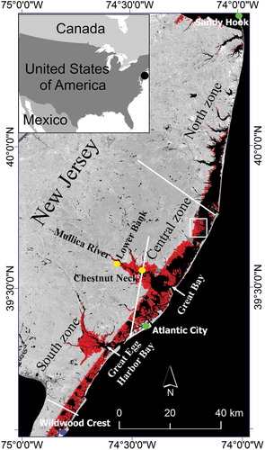
Figure 2. Hurricane Sandy surge flooding extents as obtained from COSMO-SkyMed (COSMO) and TerraSAR-X (TSX) radar images. (a) Surge extent using National Oceanic and Atmospheric Administration (NOAA) model and Atlantic City water levels; (b)–(f) surge flood extents in green on different dates of radar data. The extent of coverage of each radar collection is shown by the dotted white line on the respective dates. The background is the COSMO image of 30 August 2011. Coverage extent is the same as in Figure 1.

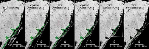
Figure 3. Surge persistence maps based on the commonality of synthetic aperture radar coverage for the central (a) and southern (b) zones (see Figure 1). Note the different compositions of surge persistence in each zone. The background is the COSMO image of 30 October 2012. See supplemental Figure S4 (a) for the northern zone.

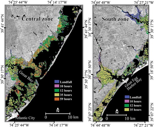
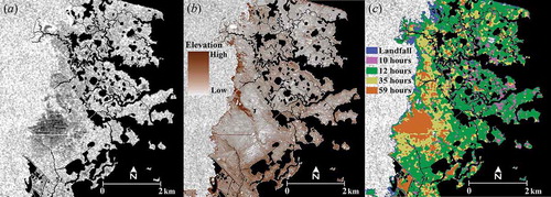
Figure 4. (a) 31 October 2012 synthetic aperture radar image, (b) topography in the depiction (the approximate range is 0.9 m (high) to 0.3 m (low)), and (c) flood persistence map. The white rectangle on Figure 1 shows the location of this area.

2. Objectives

In this study, multiple SAR images collected over a short time period following Hurricane Sandy landfall were used to extend the single surge extent to surge persistence as an indicator of possible surge impact to coastal marshes. Our objectives for this study were to:

• create surge extent maps with a progression of SAR images;

• create surge persistence maps from time-lapse SAR flood extents;

• create marsh condition change maps with optical image data; and

• determine whether a causal link exists between surge persistence and marsh condition change.

3. Study area

The study area for mapping Hurricane Sandy surge extended from Sandy Hook, NJ, in the north to Wildwood Crest, NJ, in the south, encompassing nearly the entire 127 mile (204 km) Atlantic Ocean coastline of the state (Figure 1). SAR and optical data analyses were limited to coastal marsh extracted from the NJ Department of Environmental Protection (NJDEP) Agency 2007 Land Cover data set (NJDEP 2010) lying within a 5 m elevation contour created from the US Geological Survey, National Elevation Dataset (Gesch et al. 2002; Gesch 2007) (Figure 1). Although products were created for the entire study area, research leading to the development of those products was focused on the extensive marshes of the central and southern zones (Figure 1).

3.1. The coastal wetlands of NJ

The coastal wetlands of NJ contain a mix of intertidal flats, aquatic beds, and emergent marshes (Tiner 1985). Most extensive, and the focus of this study, are the emergent marshes that are exposed to differences in salinity, as well as flood duration and frequency.

Saline marshes (approximately 18–30 practical salinity units (PSU)) dominate the coastal lagoon (water between barrier islands and mainland) back-barrier marshes. Daily tidal flushing of the low marsh lying along the shorelines produces a tall form (approximately 1 m or greater) of smooth cordgrass (Spartina alterniflora). High (platform) marsh, situated above the low marsh, is flooded less often, promoting a change that is most often exhibited as the short-form smooth cordgrass (approximately 0.5 m or less) (Tiner 1985; Ornes and Kaplan 1989). While Spartina patens and Distichlis spicata marsh grasses can occur as scattered stands (Tiner 1985), short-form smooth cordgrass dominates the high marsh.

Brackish marshes (5–18 PSU) occur landward of saline marshes likely dominating the middle reach of Great Bay and most of Great Egg Harbor Bay estuaries. Fresh estuarine marshes (0.5 and 5 PSU) primarily occur at the extreme upper reaches of the Great Bay and Great Egg Harbor Bay estuaries (Tiner 1985).

4. Data and methods

4.1. Coastal water levels

We used data from two NOAA hydrograph stations along the NJ coast, Atlantic City in central NJ, and Sandy Hook in northern NJ. The coastal water-level records were obtained from the NOAA Centre for Operational Oceanographic Products & Services (NOAA CO-OPS 2012). The Atlantic City (AC) station was used as our primary water-level reference (Table 1; Figure S1(a), S refers to supplemental; and Figure 1 for station location) because of its location near to Sandy landfall.

Table 1. Synthetic aperture radar data characteristics and acquisition times and water levels recorded at the National Oceanic and Atmospheric Administration (NOAA) Atlantic City station. The water level was 1.87 m at 24:00:00 UTC when Hurricane Sandy made landfall on 29 October 2012.

Period	Satellite	Date acquired	Time UTC	Spatial resolution (m)	Mode	Incidence angle (º) – near and far range and midpoints	Orbit	NOAA station: Atlantic City water level (NAVD 88 (m))
Before Hurricane Sandy landfall	TSX	16 December 2010	22:50	Up to 18	ScanSar	31.70	Ascending	0.03
	COSMO	27 August 2011	10:42	30	ScanSARWide	45.49; 52.28	Ascending	0.52
	TSX	30 August 2011	11:04	Up to 18	ScanSar	31.74	Descending	0.47
After Hurricane Sandy landfall	COSMO	30 October 2012	10:02	30	ScanSARWide	33.32; 43.37	Ascending	0.63
	TSX	30 October 2012	11:39	Up to 18	ScanSar	31.66	Descending	0.98
	COSMO	31 October 2012	10:44	30	ScanSARWide	33.28; 43.35	Ascending	0.66
	TSX	1 November 2012	11:04	Up to 3	Strip	35.99	Descending	0.52
	TSX	8 November 2012	22:51	Up to 18	ScanSar	31.81	Ascending	−0.09

COSMO, COSMO-SkyMed; TSX, TerraSAR-X; UTC, Coordinated Universal Time; NAVD88, North American Vertical Datum of 1988.

In addition to the NOAA coastal tide stations, we used water-level and salinity data from two hydrologic stations operated by the NOAA Jacques Cousteau National Estuarine Research Reserve System (NERRS) positioned about 9 km upstream (Chestnut Neck (CN)) and about 21 km upstream (Lower Bank (LB)) from the mouth of Mullica River (Figure 1; Table 2) (NERRS, 2013). Although inter-calibrated, the NERRS water-level recordings are not tied to a vertical datum, thereby preventing direct comparison to the AC station; however, changes in water levels at the stations are comparable. For example, the AC, CN and LB hydrographs recorded the highest water levels within the study period at landfall (Table 2, Figures S1(a) and S1(b)).

Table 2. Salinity and water levels from the two National Oceanic and Atmospheric Administration (NOAA)-National Estuarine Research Reserve System (NERRS) sampling stations.

SAR	†Date acquired	Time (UTC)	Length of time after landfall (hours)	NOAA-NERRS station
				Chestnut Neck		Lower Bank
				Salinity (PSU)	Water level (m)	Salinity (PSU)	Water level (m)
Reference:
Hurricane Sandy landfall	29 October	24:00	0	28.20	3.41	22.6	3.63
COSMO	30 October	10:02	10	26.50	2.86	20.2	3.61
TSX	30 October	11:39	12	26.00	2.83	17.5	3.45
COSMO	31 October	10:44	35	12.70	2.05	3.9	2.02
TSX	1 November	11:04	59	9.60	1.82	1.3	1.78
TSX	8 November	22:51	239	14.70	2.54	6.7	2.56

SAR, synthetic aperture radar; COSMO, COSMO-SkyMed; TSX, TerraSAR-X; UTC, Coordinated Universal Time; PSU, practical salinity units. ^†All dates were in 2012.

4.2. Image data

4.2.1. TSX and COSMO SAR image collections

TSX and COSMO X-band collection modes and times before and after Hurricane Sandy landfall are listed in Table 1. We used available pre-hurricane reference SAR images with a near consistency in seasonality with Hurricane Sandy. The single COSMOS reference image collected on 27 August 2011 had a higher incident range (10º) than the post-hurricane target COSMOS images. Additionally, the reference COSMOS image and the TSX reference image on 30 August 2011 were collected during elevated sea levels associated with Hurricane Irene that made landfall in North Carolina on 27 August 2011 (Table 1). Even though reference images collected with the same incident range and during low sea levels are preferred (Ramsey, Rangoonwala, and Bannister 2013), lack of better alternative reference images resulted in the use of the pre-hurricane August images.

4.2.2. Optical imagery collections

Three SPOT 5 images (10 m ground resolution, near 18º off-nadir) covering most of the study area were the only high- to moderate-spatial resolution (≤30 m) optical images collected within a couple of months of landfall that had minimal cloud coverage (Table 3). See Table 3 for water levels specific to SPOT collections. The post-landfall SPOT images were collected on 30 December 2012 within the marsh senescent period. Because the onset of senescence reduces the ability to link marsh dieback to surge, daily MODIS Aqua and Terra imagery (about 232 m ground resolution) were acquired to provide an additional assessment of marsh change before and after the hurricane. MODIS images used in the marsh condition change analysis were collected at low water levels as recorded at the AC station.

Table 3. Optical Satellite Pour l’Observation de la Terre (SPOT) 5 multispectral data characteristics and acquisition times and water levels from two National Oceanic and Atmospheric Administration (NOAA) hydrograph stations.

Period	Coverage	^†Date acquired	Time (UTC)	Water level (NAVD88 (m))	NOAA station
Before Hurricane Sandy landfall	Northern	17 September	10:02	0.44	Sandy Hook
	Central	13 October	15:30	−0.72	Atlantic City
	Southern	13 October	15:30	−0.72	Atlantic City
After Hurricane Sandy Landfall	Northern	30 December	15:27	0.31	Sandy Hook
	Central	30 December	15:27	0.16	Atlantic City
	Southern	30 December	15:27	0.16	Atlantic City

UTC, Coordinated Universal Time; spatial resolution, 10 m. ^†All dates were in 2012; NAVD88, North American Vertical Datum of 1988.

4.2.3. SAR data calibration

The COSMO data were Geocoded Ellipsoid Corrected (GEC) HDF5 level 1C products and one 1C GeoTIFF product. The TSX data were acquired in Enhanced Ellipsoid Corrected (EEC) level 1B format. All COSMO and TSX data were radiometrically calibrated to backscattering coefficient sigma naught (σ°) to allow image-to-image comparability. Two COSMO and all TSX images were processed using the Universal Transverse Mercator (UTM) projection and calibrated to σ° by using the Next European Space Agency (ESA) SAR Toolbox (NEST), which is an ESA open source toolbox for processing SAR data. The COSMO image in the 1C GeoTIFF format was calibrated to σ° by using equations given in e-GEOS (2015).

4.2.4. SPOT and MODIS data calibration and correction

The SPOT at-sensor radiance data were converted to marsh canopy reflectance with the Atmospheric and Topographic Reduction (ATCOR) radiative transfer model (Richter and Schläpfer 2011) applied within PCI Geomatica®. A maritime scattering phase function was chosen to represent the atmospheric composition at the times of the SPOT image collections. Horizontal visibility, also required for the atmospheric correction, was obtained in two steps. First, the total atmospheric optical depth was calculated as the sum of the optical depths related to Mie and aerosol scattering obtained from Multi-sensor Aerosol Products Sampling System (NASA 2015) and optical depth related to Rayleigh scattering estimated at standard atmospheric conditions (Elterman 1970). Next, the total optical depth was transformed to horizontal visibility estimates at 0.55 micrometre (µm) (Elterman 1970; Ramsey and Nelson 2005).

The Time Series Product Tool (TSPT) was used to temporally process daily MODIS Terra MOD09 and Aqua MYD09 atmospherically corrected surface reflectance products (Vermote and Kotchenova 2008) into daily normalized difference vegetation indices (NDVIs) (Rouse et al. 1973). Developed at the National Aeronautics and Space Administration (NASA) John C. Stennis Space Centre, TSPT was used to remove inferior MODIS surface reflectance data (e.g. from clouds and poor viewing geometry), compute NDVIs, fuse Aqua and Terra data into composited daily NDVI products, remove abnormal data spikes caused by residual noise, perform data void interpolation for null data values, and smooth NDVI values in the time series by using a Savitzky–Golay curve fitting algorithm. Refer to (Ramsey et al. 2011b) for additional information.

4.2.5. Rectification, registration, and compositing of image data

COSMO, TSX, and SPOT images were registered to USGS digital orthophoto quarter quadrangles (DOQQs) with a stated root mean square error of no more than 7 m. The rectification errors to the DOQQs were most often less than 0.2 pixels.

4.3. Mapping surge extent

Post-hurricane surge persistence mapping included tidal periodicities and amplitudes that could have flushed back-barrier marshes (those lying behind the barrier islands and within the lagoon). To assess the post-hurricane tidal flushing likelihood, we considered water levels and salinities, the pattern of progressive flood maps, topographic controls, and relative backscatter attenuation as an indication of marsh flooding (e.g. Dobson, Pierce, and Ulaby 1996). Direct interpretation of backscatter decrease with flood depth increase depends on X-band perceiving marsh flooding at all depths. Given the pervasiveness of short-form marsh within the study area, we consider that shallow marsh flooding was well mapped except possibly where taller marsh or marsh forming thick mats tended to obscure X-band perception of shallow flooding.

4.3.1. Surge extent at Hurricane Sandy landfall

Methods documented by NOAA were used to produce a first-order approximation based on water stage and coastal elevations to calculate surge extent at the time of Hurricane Sandy landfall (Marcy et al. 2011). The calculation set the pixel as either flooded or non-flooded by comparing the topographic elevation to the NOAA stage recording from AC (Figure 2(a)).

4.3.2. SAR surge extent mapping

In order to maximize the detection of persistent surge flooding as time increased and sub-canopy flood depth decreased after landfall, the backscatter of the reference image (non-flooded) collected before landfall was compared to that of the target image (possibly flooded) collected during and after the flood event (Klemas 2009; Rami’rez-Herrera and Navarrete-Pacheco 2012). To perform the calculation, the σ⁰ data in decibels (dB) were converted to amplitude and a change detection algorithm applied in PCI Geomatica® (Ramsey et al. 2011b, 2012, 2013).

To help alleviate change artefacts not related to flooding, global minimum change thresholds were applied to each SAR image. Threshold determination was isolated to the marshes without open water to ensure the selected thresholds emphasized backscatter attenuation caused by sub-canopy flooding with the X-band systems. Thresholds from the 10 and 12 h SAR collections were associated with high flood versus non-flood marsh amplitude contrasts. The relatively decreased depths of flooding present at the 35 and 59 h SAR collections resulted in lower and more spatially variable flood versus non-flood contrasts. Added to this, possible flooding in the pre-hurricane reference images used in the 35 and 59 h surge extent calculation and a higher relative incidence range of the reference image used in the 35 h calculation could have degraded detection performance. While reference image flooding could lower performance, the shallower incident angle effect on flood detection performance is less clear. To help minimize possible detection error, particularly related to the incidence angle difference, thresholds were chosen in these two latter time periods that approximated the midpoints in the spatial continuum of high to low contrast. In effect, marsh with the higher likelihood of sub-canopy flooding was retained, whereas marsh with the lower likelihood of sub-canopy flooding was eliminated.

4.4. Surge persistence

In order to interpret the intersection of calculated surge extent as persistence, the SAR spatial extents were overlain and three separate zones defined such that each encompassed a unique, spatially uniform sequential coverage (Figures 1, 2(b)–2(f)). The timeline of surge extents included the time-zero landfall extent calculated with the NOAA method and SAR-based extents calculated at 10, 12, 35, and 59 h after landfall. The northern zone included SAR collections at 10, 35, and 59 h, the central zone 10, 12, 35, and 59 h, and the southern zone 10, 12, and 35 h after landfall.

4.4.1. Calculation of surge persistence per zone

In this study, ‘persistence’ refers to the number of consecutive times starting at landfall through the 1 November SAR collection from which a marsh location or image pixel was determined to be flooded. Calculation of the spatial correspondence of flooding through time from landfall to 59 h after landfall used in-house scripts based on PCI Geomatica® coding syntax to calculate the spatial juxtaposition of each subsequent flood extent to the previous flood extent per zone.

4.4.2. Assessment of surge persistence

Interpretation of the spatial correspondence in flooding state over time depends on whether evidence indicates repeatedly observed flooding or persistence of surge flooding from landfall. Interpretation was aided by overlaying the surge persistence calculation results on coastal topographic maps. For example, in regions of high persistence, we looked for topographic controls such as barriers that restricted flow or highs and lows of marsh topography that promoted or restricted pooling. The comparisons provided evidence for post-surge persistence through the observed 35 and 59 h periods.

4.5. Mapping marsh condition

Marsh condition change analyses excluded permanent open water and cloud and cloud shadows. Following an approach similar to Ramsey et al. (2012), NDVI was used to determine condition change in marsh greenness (i.e. condition) after the storm. The natural variability of marsh greenness was taken into account by including both pre- and pre- to post-NDVI changes in the k-means unsupervised classification (e.g. Ramsey et al. 2012) using ERDAS IMAGINE®. The pre-NDVI and change-NDVI ranges were approximately equalized before classification by multiplying the change-NDVI magnitudes by 10. To minimize the influence of sub-canopy marsh flooding on the classification, we excluded pixels with NDVI less than 0.0, or a combined modified normalized water index (MNDWI) (Xu 2006) less than 0.1 and NDVI less than 0.2. Of the 400.9 km² of marsh within the SPOT observed area, 322.1 km² (85.2%) were assessed for condition change. The classification produced four marsh condition change classes (i.e. low, moderate, high, and severe).

A second comparison used the daily MODIS NDVI data collected on 22–26 October 2012, a few days before landfall, and on 9–13 November 2012, within two weeks after landfall. To avoid issues associated with marsh–water and marsh–upland boundaries, MODIS pixels containing less than 50% marsh were excluded from change analyses. Marsh condition changes that were less than −0.011 (on a native NDVI scaling of −1.000 to +1.000) were eliminated from analyses.

4.6. Association of surge persistence and marsh condition

The spatial association between the surge persistence and marsh condition map used a cross-correlation approach in PCI Geomatica®. Inputs to cross-correlation procedure were five surge persistence durations ranging from landfall (i.e. 0 h) to 10, 12, 35, and 59 h after landfall and marsh condition change with the four severity classes. Coincidence values were aggregated based on the cross-correlation matrix, and a four-category map was created that showed the relation of surge persistence to marsh condition change.

5. Results

5.1. Maps showing extent of storm surge and surge persistence

Figure 2(a)–2(f) are maps showing the extent of flooding during and post-Hurricane Sandy. Landfall surge calculated with the NOAA elevation-driven model covered 39,247 ha within coastal marsh (Table S1 and depicted in Figure 2(a)). By the time of the first available SAR collections at 10 and 12 h after landfall, surge coverage of the marsh had decreased by 14 and 21% in the central zone, respectively, and by 16 and 39% in the southern zone, respectively (Table S1; Figure 2(b) and 2(c)). At 35 h after landfall, marsh flooding had decreased up to 41% in the central zone and remained fairly constant relative to the landfall surge extent in the southern zone (Table S1, Figure 2(d)). At 10 and 35 h, the northern surge extent was 45% of the landfall extent. Flood extent at 59 h after landfall had further decreased by another 20% in the central zone and 26% in the northern zone since 35 h (Table S1; Figure 2(e)).

Surge extents were most clearly distinguished on the SAR images at 10 and 12 h after landfall; however, the 12 h SAR image flood versus non-flood delineation was hampered by wind-roughened water surfaces (Figure S2(c) and S2(d)). Although exclusion of permanent open water minimized confusion among the wind-roughened water surfaces (Ramsey et al. 1994), at flood heights approaching the top of the marsh, wind disturbance of the water surface could increase backscatter, thereby leading to misinterpretation of the flooded as non-flooded marsh (Ramsey et al. 2012).

The 10 and 12 h SAR-based flood extents occurred on the first rising tide following landfall, as depicted in the AC hydrograph (Figure S1(a)). The Great Bay hydrographs, however, show that both 10 and 12 h SAR collections remained at high water levels, only slightly responding to the semi-diurnal tidal period (Table 2; Figure S1(b) and S1(c)). The continuation of high water levels and surge salinities just inside Great Bay indicated that elevated-salinity surge waters were retained within the bay and most likely within the lagoon. Although salinity recordings suggest that lagoon surge waters had not yet begun to mix widely with freshwater runoff or coastal waters, the 35 cm tidal rise from 10 to 12 h after landfall recorded at AC was expressed in the respective SAR image collections (Figure S3).

At 35 and 59 h after landfall, water levels decreased to typical levels and salinities had dropped to below pre-hurricane ranges. Although water-level heights at 35 h were higher than at 10 h according to AC tide recordings, Great Bay water levels showed the reverse. Marsh flooding at 10 h clearly was more extensive than at 35 h, and as indicated by the SAR flood mapping, water levels at 59 h were lower at both AC and Great Bay stations, aligning with the lowest calculated areal flooding used in the persistence calculation (Table S1). SAR mapping showed only minor and scattered pooling at 239 h past landfall when water levels were low, reinforcing the flood mapping performance (Figure 2(f); Table 1).

5.2. Surge persistence

Surge persistence maps were created for all three zones by using a combination of surge and flood extents (Figure 3(a), 3(b), and S4(a)). Modifications were made in the script logic to calculate persistence based on inspection of the input extent maps and products. For example, misclassification of flooded marsh as non-flooded caused by wind roughening of the water surface (Figure S2(c) and S2(d)) was reinterpreted within the script logic by taking into account previous and subsequent flood occurrences.

5.2.1. Comparing persistence and topography

A comparison of topography and surge spatial alignment provided validation to persistence maps in the northern end of the central zone (Figure 4(a)–(c)). The 31 October 2012 SAR image illustrated the continued low backscatter from marsh located at the inland extent of the marsh platform (Figure 4(a)). The topographic surface identified this marsh region as a depression, bounded by upland to the west and a ridge to the east generally aligned with the coast (Figure 4(b)). The calculated persistent well reflects the contour of the depression (Figure 4(c)). A likely explanation is that surge waters high enough to top the ridge were trapped and persisted. Observed flood persistence results also confirm that tidal heights at 35 and 59 h following the surge-elevated period did not flood the extensive marshes seaward of the ridge. Lack of flooding occurred even though these seaward marshes were at relatively low elevations. Figures S5 and S6 provide similar graphical comparisons at locations south of those in Figure 4.

5.3. Marsh condition change

Good visual agreement is shown in the SPOT and MODIS spatial pattern of marsh condition change in the central and southern zones (Figure 5(a)–5(d)). Within that overall agreement, differences in spatial resolutions, most apparent in the back-barrier marshes lying between Great Bay and Great Egg Harbor Bay, led to some local-scale differences in calculated condition change. Outside of that spatially complex marsh region, one contiguous area of marsh surrounding the north of Great Bay (Figure 5(a)–5(c)) exhibited non-coincidence that was less likely related to differences in spatial resolution. Lack of sufficient information, however, hindered speculation as to what caused that difference.

Figure 5. (a) and (b) show marsh condition change maps generated using optical Satellite Pour l’Observation de la Terre (SPOT) data; (c) and (d) show marsh condition change maps generated using optical satellite Moderate Resolution Imaging Spectroradiometer (MODIS) data. The arrow in Figure 5(a) and 5(c) denotes a region of non-coincidence in SPOT and MODIS marsh condition mapping. Zone locations are shown on Figure 1 and coverage extents are the same as in Figures 3 and 6. See supplemental Figure S4 (b) for northern zone SPOT marsh condition map.

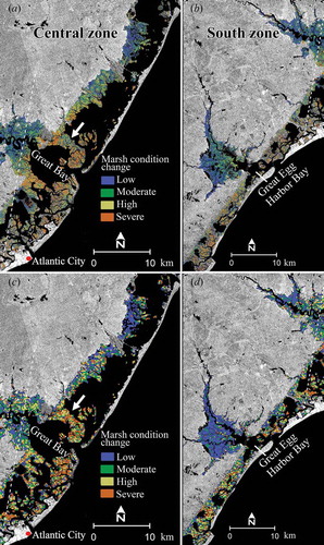
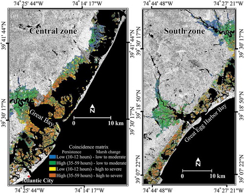
Figure 6. Coincidence matrix showing spatial association between surge persistence and Satellite Pour l’Observation de la Terre (SPOT) marsh condition change maps for (a) central zone and (b) southern zone. Zones are shown on Figure 1. The background is the COSMO image of 31 October 2012. See supplemental Figure S4 (c) for northern zone coincidence matrix.

Although difference in collection dates prevented direct comparison of magnitudes, NDVI patterns in class magnitude and membership showed close alignment of SPOT-based and MODIS-based marsh condition results. In both, NDVI means progressively increased from the low to severe class and the low-change class dominated (Table 4). In addition, the correspondence between SPOT and MODIS mean NDVI changes was high (R² = 0.99, n = 4 change classes) with a constant gain of 1.42 ± 0.11 (±standard error) and offset of 0.156 ± 0.011 (SAS® Enterprise). Close similarity of the condition change spatial distributions and the trends in pre- and post-surge SPOT and MODIS marsh condition class means and changes provided substantial corroborative evidence that the SPOT NDVI change map offers a useful local-scale representation of marsh condition change due to Hurricane Sandy.

Table 4. Optical data marsh condition change normalized difference vegetation index (NDVI) classes and statistics.

Sensor	Marsh condition change	Area (km^2)	Coverage (%)	Mean Pre-hurricane NDVI	Standard deviation pre-hurricane NDVI	Mean post-hurricane NDVI	Standard deviation post-hurricane NDVI	†Mean NDVI change	Standard deviation NDVI change
SPOT	Low	124.30	38.60	0.32	0.06	0.11	0.07	0.21	0.05
	Moderate	66.91	20.80	0.38	0.04	0.11	0.07	0.27	0.03
	High	75.01	23.30	0.39	0.05	0.08	0.07	0.31	0.03
	Severe	55.89	17.40	0.43	0.06	0.05	0.09	0.38	0.05
MODIS	Low	150.10	45.90	0.47	0.07	0.43	0.07	0.04	0.02
	Moderate	61.33	18.80	0.50	0.06	0.42	0.07	0.08	0.01
	High	68.95	21.10	0.51	0.07	0.40	0.07	0.10	0.01
	Severe	46.66	14.30	0.53	0.08	0.38	0.08	0.16	0.03

^† Mean NDVI change is the mean difference between pre- and post-hurricane NDVI values; SPOT, Satellite Pour l’Observation de la Terre; MODIS, Moderate Resolution Imaging Spectroradiometer.

The highest condition changes occurred within the central zone to the north of the Hurricane Sandy landfall track and just outside the mouth of Great Bay (Figure 5(a)). Both the Great Bay and Great Egg Harbor Bay riverine estuaries dominantly showed the lowest changes, particularly in the landward extremes (Figure 5(a) and 5(b)). Low change also occurred in the furthest northern back-barrier marshes of the central zone (Figure 5(a)). That trend of low marsh condition change also typified the scattered pocket marshes extending northward along the NJ coast (Figure S4(b)). South of Great Bay, the back-barrier marshes exhibited a mixture of marsh condition changes, with pockets of high to severe change scattered within areas of low change (Figure 5(b)).

5.4. Linking marsh condition change to persistence

In the central zone, low persistence was nearly equally associated with low and high marsh change, and high persistence was associated about 13% more often with high than low change (Figure 6(a), Table 5). High persistence and marsh change were concentrated with marshes extending outward from the mouth of Great Bay (Figure 6(a)). That high correspondence extended northward to a section of back-barrier marshes exhibiting predominantly low persistence and low change (Figures 6(a) and S5(b)). In the northernmost marshes of the central zone, the alignment was again high except in the interior marshes, where high persistence had been documented (Figures 6(a) and 4(c)). Further north, high surge persistence was dominantly associated with low change (Figure S4(c); Table 5).

Table 5. Coincidence matrix result for the surge persistence and marsh condition change maps. The reference surge persistence (landfall), as well as persistence 10 and 12 h after landfall, were categorized as low persistence, and 35 and 59 h after landfall were categorized as high persistence. The low and moderate marsh condition changes were depicted as low, and the high and severe marsh condition changes as high. to describe the matrix associations. The same colours are used in Figure 6 to illustrate spatial distribution. The ‘Total’ row in each zone shows the total area in hectares (ha) represented by each colour per zone.

			Surge persistence (ha)
Coverage			Reference	10 h	12 h	35 h	59 h
	Marsh change			Low/High
Northern zone	Low	Low	395.90	23.09	N/A	603.42	207.96
	Moderate		180.62	6.32	N/A	135.65	31.49
	High	High	201.75	6.25	N/A	110.20	27.60
	Severe		219.07	7.42	N/A	81.87	51.28
	Total			605.98			978.52
				434.39			270.95
Central zone	Low	Low	194.32	168.96	1284.53	1242.56	706.85
	Moderate		134.14	116.04	947.67	890.50	548.19
	High	High	199.23	167.49	1184.65	1269.26	899.10
	Severe		231.20	148.01	803.12	923.45	767.18
	Total				2845.66		3388.10
					2733.70		3858.99
Southern zone	Low	Low	1617.43	577.99	981.28	4131.49	N/A
	Moderate		584.99	223.98	454.83	231952	N/A
	High	High	517.79	199.30	390.30	2186.82	N/A
	Severe		386.27	115.57	221.33	1453.97	N/A
	Total				4440.50	6451.01
					1830.56	3640.79

N/A, no image coverage.

In the southern zone, low persistence was more than twice as likely to be associated with low change, and high persistence (limited to 35 h) was about 1.75 times as likely to correspond to low change (Figure 6(b), Table 5). South of Great Bay before reaching Great Egg Harbor Bay, spatial distributions of flood persistence and condition change in the back-barrier marshes, showed scattered correspondence within marshes calculated to have undergone high surge persistence but little change in vegetation canopy greenness. South of Great Egg Harbor Bay, back-barrier marshes exhibited fairly equal proportions of high change and high persistence and low change and high persistence. Marshes within Great Bay and Great Egg Harbor Bay exhibited high disagreement that was dominated by low change associated with high persistence (Figure 6(a) and 6(b)). Further upstream, however, both bays exhibited low change and low persistence.

6. Discussion

6.1. Surge persistence

Although qualitative, the spatial alignment of discernible features in the topographic and calculated persistence maps is visually evident in marshes of the central zone surrounding and to the north of Great Bay. Outside of clearly defined depressions and surrounding ridges (Figures 4, S5, and S6), however, evidence for surge persistence is not as visually apparent. Along-shore ridges, particularly noticeable in the central zone, suggest impedance of tidal flow into the interior marshes at low tides (e.g. Figure S6 (a)). One complication of this interpretation is the juxtaposition of low persistence (Figure S6 (b)) and the documented occurrence of taller smooth cordgrass marsh along shorelines in this area. Detection of shallow flooding 35 h after the surge may have been hampered by attenuation of the radar signal by taller marsh. If present but not detected, shallow flooding could have extended into the inner platform marsh, accounting for the detected flooding, but not observed as flooding along the shoreline. Observations related to the possibility of post-hurricane tidal flushing, however, reduce that possibility. First, tides must overcome the shoreline ridge to flush the platform marsh. Second, extensive low-lying marshes north of Great Bay without impediments to coastal flushing were flooded by neither 35 nor 59 h tides, as illustrated in Figure 4(c). Third, inspection of the 10 or 12 h SAR images (Figure S3) indicates that marshes just to the south of Great Bay were less prone to flushing than to the north. These observations suggest that the flood persistence maps provide a good representation of surge persistence in back-barrier marsh surrounding and to the north of Great Bay.

We also examined the possibility that sub-canopy flooding seen in the lagoon back-barrier marshes on the 59 h collection was caused by tides after SAR collection at 35 h. The 35 h collection occurred on rising tides of the major components of the semi-diurnal tidal period (Figure S1(a)). From the Great Bay water levels and SAR-based flood extents, we know that although AC tide levels suggested similar heights at 10 and 35 h past landfall, water levels in the lower estuary and lagoon were in fact lower at 35 h past landfall (Table 2; Figure S3). Also, the Great Bay hydrograph (CN) shows that the SAR collection at 35 h was within 3 cm of peak flooding (Figure S1(b)). It is possible that platform marshes were partially flooded after the 35 h SAR collection on what remained of the rising tide; however, the available information minimizes that possibility.

Evidence including compiled topographic maps, water-level recordings, and the SAR images suggests that most marshes along the NJ Atlantic coast were not tidally flushed 35 and 59 h after landfall. The persistence calculated from flood extent maps created from a landfall NOAA-based estimate and subsequent SAR images provides a meaningful representation of the duration of exposure of the marshes to elevated-salinity surge waters. The persistence also infers the length of time the marshes were flooded as related to the possibility of waterlogging.

6.2. Linking the change in marsh condition to persistence

Even though noticeable differences occurred, there was substantial agreement between the SPOT and MODIS NDVI change products that provided justification for use of the SPOT marsh condition change and TSX and COSMO surge persistence as an indication of Hurricane Sandy marsh impact.

There was a distinct correspondence pattern to the marsh condition change and surge persistence distributions. High change and persistence correspondence was dominantly centred on marshes surrounding and somewhat to the north of Great Bay. Mixed within these regions of high persistence and change correspondence were marshes exhibiting high condition change and low flooding persistence. Their intertwined spatial occurrence and common association with high change suggested an inconsistency in persistence. Much of this seeming inconsistency can be explained as uncorrected wind roughening of the water surface at high water (Figures S2(c) and (d)) and possible non-penetration of the radar to the shallow sub-canopy flooding along shorelines occupied by tall form smooth cordgrass marsh (Figure S6(b)).

On the other hand, marshes of high persistence and low change were found to dominate interior Great Bay and Great Egg Harbor Bay marshes and to exhibit a near equal dominance in back-barrier marshes lying south of Great Bay. In one area of disagreement between SPOT and MODIS condition mapping just to the north of Great Bay (Figure 5), MODIS condition change would have aligned with high surge persistence. Conversely, large patches in back-barrier marshes north of Great Bay showed good MODIS and SPOT agreement. One patch of low change was located in platform marsh of documented high-surge persistence (Figure 4(c)). In other words, both high persistence and low change were fairly well established. Farther to the south of Great Bay, the patchiness of persistence and change resulted in a highly irregular correspondence landscape, suggesting heterogeneity of marsh structures and possibly types.

Even though persistence coincided with calculated change in the upper reaches of Great Bay and Great Egg Harbor Bay, extensive and uniform non-correspondence existed in the lower reaches of both bays. This non-correspondence suggests that either the change or persistence calculation is incorrect, that the marshes are more resistant to elevated-salinity waters, or that the documented flow of freshwater into these marshes forestalled or mitigated detrimental impact. Both MODIS and SPOT change analyses determined little change in these bays; however, MODIS change reflected more discontinuity in the lower Great Bay marshes. Even unrealistically increasing the thresholds in the SAR-based surge extent calculation would not have eliminated the high surge persistence calculated in these bays. Although information is lacking to determine a conclusive scenario, it is possible that the surge-associated elevated salinity was mitigated by freshwater input lessening or eliminating damage that occurred in the lower Great Bay marshes.

7. Conclusion

Hurricane Sandy surge extent and persistence along the 204 km NJ Atlantic coast was related to change in the condition of the back-barrier lagoon and estuarine marshes. Analyses of SAR showed that extensive and nearly uniform surge flooding of the coastal marshes occurred for the first 12 h after landfall. Flood extents calculated at 35 and 59 h after landfall were interpreted to primarily consist of the persistent early surge flooding in the back-barrier lagoon marshes. The change in marsh condition was calculated with SPOT and MODIS optical satellite data collected before and after the hurricane. Widespread agreement between the two condition maps allowed assessment of a possible link between surge persistence and marsh condition change products.

Results showed that back-barrier marshes stretching about 20 km north of the Hurricane Sandy landfall track experienced high surge persistence and suffered high condition change. Stretching for another 20 km just north of that high-impact region, back-barrier marsh exhibiting low condition change was largely aligned with low surge persistence. A trend of low marsh condition change associated with high and low surge persistence typified post-surge history and response in the scattered pocket marshes extending further northward along the NJ coast. South of the landfall track, back-barrier marsh became less contiguous and more spatially complex and exhibited near equal amounts of high persistence associated with low and high condition change. A different post-surge history was reflected by estuarine marshes within Great Bay and Great Egg Harbor Bay. These marshes were associated with high persistent flooding but exhibited low change. It is possible that the timely injection of high freshwater runoff between 12 and 35 h after landfall averted the high impact suffered by many back-barrier lagoon marshes. Overall, the independent calculation of SAR-based surge persistence and optical-based marsh condition change revealed an extended region of high surge-related marsh impacts north of the Hurricane Sandy landfall track. Outside of this high impact region, distinct patterns in persistence and condition were possibly related to freshwater mitigation, heterogeneity of marsh structure, and possible differential resilience. Our approach and products provide resource management with a new and effective strategy for identifying and responding to surge persistence latent impacts to coastal resiliency.

Acknowledgements

Partial support for this work was provided under US Geological Survey Hurricane Sandy Supplemental Funds (AE03FBK, GX13SC00FBK). Access to TerraSAR-X data was provided through a grant (COA2070) from the German Aerospace Center (DLR). Part of this work was performed under a US Geological Survey and University of Louisiana at Lafayette Cooperative Ecosystem Studies Units contract. Work by Computer Sciences Corporation, Inc., on this project was supported by NASA at the John C. Stennis Space Center, Mississippi, under contract NNS10AA35C. This project leveraged MODIS data products developed in support of the USDA Forest Service ForWarn system. We thank Dirk Werle of ÆRDE Environmental Research, Canada, for providing critical background information for this manuscript. Any use of trade, firm, or product names is for descriptive purposes only and does not imply endorsement by the US Government.

Disclosure statement

No potential conflict of interest was reported by the authors.

Supplemental data and underlying research materials

The underlying research materials for this article can be accessed at http://dx.doi.org/10.1080/01431161.2016.1163748 / Materials provided Table S1, and Figures S1, S2, S3, S4, S5 and S6.

Additional information

Funding

This work was supported by US Geological Survey Hurricane Sandy Supplemental Funds (AE03FBK, GX13SC00FBK). Access to TerraSAR-X data was provided through a grant (COA2070) from the German Aerospace Center (DLR).

References

- ÆRDE Environmental Research. 2015. “Literature Review: Floods.” 103 p. Halifax, Nova Scotia:Department of Natural Resources Canada.
- Ajmar, A., P. Boccardo, F. Disabato, F. G. Tonolo, F. Perez, and G. Sartori. 2008. “Early Impact Procedures for Flood Events February 2007 Mozambique Flood.” Italian Journal of Remote Sensing 40: 65–77. doi:10.5721/ItJRS20084036.
- Bayley, P. B. 1995. “Understanding Large River: Floodplain Ecosystems.” Bioscience 45: 153–158. doi:10.2307/1312554.
- Blake, E. S., T. B. Kimberlain, R. J. Berg, J. P. Cangialosi, and J. L. Beven II. 2013. “Tropical Cyclone Report: Hurricane Sandy. (AL182012) 22 – 29 October 2012.” 157 p. Accessed December 13, 2015. http://www.nhc.noaa.gov/data/tcr/AL182012_Sandy.pdf
- Dobson, M., L. Pierce, and F. Ulaby. 1996. “Knowledge-Based Land-Cover Classification Using ERS-1/JERS-1 SAR Composites.” Institute of Electrical and Electronics Engineers Transactions on Geoscience Remote Sensing 34: 83–99. doi:10.1109/36.481896.
- Donlon, C. 2010. ESA Storm Surge (eSurge) Demonstration Service: User Requirements Document. Noordwijk, The Netherlands: European Space Agency European Space Research and Technology Centre, 113 p. Accessed December 13, 2015. http://due.esrin.esa.int/files/eSurge-URD-ver1.0-rev-1.0-20101008.pdf.
- e-GEOS. 2015. “COSMO –SKYMED Image Calibration.” Accessed December 13, 2015. http://www.e-geos.it/products/pdf/COSMO-SkyMed-Image_Calibration.pdf
- Elterman, L. 1970. “Vertical-Attenuation Model with Eight Surface Meteorological Ranges 2 to 13 Kilometers.” 56 p. Bedford, MA: Air Force Cambridge Research Laboratories.
- Gesch, D., M. Oimoen, S. Greenlee, C. Nelson, M. Steuck, and D. Tyler. 2002. “The National Elevation Dataset.” Photogrammetric Engineering & Remote Sensing 68: 5–11.
- Gesch, D. B. 2007. “The National Elevation Dataset.” Chap 4 in Digital Elevation Model Technologies and Applications: The DEM User’s Manual, 2nd ed., edited by D. Maune, 99–118. Bethesda, MD: American Society for Photogrammetry and Remote Sensing.
- Hess, L., J. Melack, S. Filoso, and Y. Wang. 1995. “Delineation of Inundated Area and Vegetation along the Amazon Floodplain with the SIR-C Synthetic Aperture Radar.” Institute of Electrical and Electronics Engineers Transactions on Geoscience Remote Sensing 33: 896–904. doi:10.1109/36.406675.
- Hong, S., S. Wdowinski, and S. Kim. 2010. “Evaluation of Terrasar-X Observations for Wetland Insar Application.” Institute of Electrical and Electronics Engineers Transactions on Geoscience Remote Sensing 48: 864–873. doi:10.1109/TGRS.2009.2026895.
- Kasischke, E., K. Smith, L. Bourgeau-Chavez, E. Romanowicz, S. Brunzell, and C. Richardson. 2003. “Effects of Seasonal Hydrologic Patterns in South Florida Wetlands on Radar Backscatter Measured from ERS-2 SAR Imagery.” Remote Sensing of Environment 88: 423–441. doi:10.1016/j.rse.2003.08.016.
- Kiage, L., N. Walker, S. Balasubramanian, A. Babin, and J. Barras. 2005. “Applications of Radarsat-1 Synthetic Aperture Radar Imagery to Assess Hurricane-Related Flooding of Coastal Louisiana.” International Journal of Remote Sensing 26: 5359–5380. doi:10.1080/01431160500442438.
- Klemas, V. 2009. “The Role of Remote Sensing in Predicting and Determining Coastal Storm Impacts.” Journal of Coastal Research 256: 1264–1275. doi:10.2112/08-1146.1.
- Klemas, V. 2014. “Remote Sensing of Floods and Flood-Prone Areas: An Overview.” Journal of Coastal Research 31: 1005–1013. doi:10.2112/JCOASTRES-D-14-00160.1.
- Lang, M., P. Townsend, and E. Kasischke. 2008. “Influence of Incidence Angle on Detecting Flooded Forests Using C-HH Synthetic Aperture Radar Data.” Remote Sensing of Environment 112: 3898–3907. doi:10.1016/j.rse.2008.06.013.
- Leconte, R., and T. Pultz. 1991. “Evaluation of the Potential of Radarsat for Flood Mapping Using Simulated Satellite SAR Imagery.” Canadian Journal of Remote Sensing 17: 241–249.
- Marcy, D., W. Brooks, K. Draganov, B. Hadley, C. Haynes, N. Herold, J. McCombs, M. Pendleton, S. Ryan, K. Schmid, M. Sutherland, and K. Waters. 2011. “New Mapping Tool and Techniques for Visualizing Sea Level Rise and Coastal Flooding Impacts”. In Proceedings of Solutions to coastal disasters. Anchorage, Alaska, USA: American society of civil engineers, 474–490. Accessed October 27, 2014. http://coast.noaa.gov/slr/
- Marti-Cardona, B., J. Dolz-Ripolles, and C. Lopez-Martinez. 2013. “Wetland Inundation Monitoring by the Synergistic Use of ENVISAT/ASAR Imagery and Ancilliary Spatial Data.” Remote Sensing of Environment 139: 171–184. doi:10.1016/j.rse.2013.07.028.
- Martinis, S., A. Twele, C. Strobl, J. Kersten, and E. Stein. 2013. “A Multi-Scale Flood Monitoring System Based on Fully Automatic MODIS and Terrasar-X Processing Chains.” Remote Sensing 5: 5598–5619. doi:10.3390/rs5115598.
- Martinis, S., A. Twele, and S. Voigt. 2009. “Towards Operational near Real-Time Flood Detection Using a Split-Based Automatic Thresholding Procedure on High Resolution Terrasar-X Data.” Natural Hazards and Earth System Science 9: 303–314. doi:10.5194/nhess-9-303-2009.
- NASA. 2015. “Multi-Sensor Aerosol Products Sampling System.” Accessed December 14, 2015. http://giovanni.gsfc.nasa.gov/mapss/
- National Research Council. 2009. Mapping the Zone: Improving Flood Map Accuracy, 122 p. Washington, DC: The National Academies Press. doi:10.17226/12573.
- NERRS (NOAA National Estuarine Research Reserve System). 2013. “System-Wide Monitoring Program.” Data from the NOAA NERRS Centralized Data Management Office. Accessed December 14, 2015. http://www.nerrsdata.org/
- NJDEP (New Jersey Department of Environmental Protection). 2010. “2007 Land Use/Land Cover Update.” Accessed January 11, 2015. http://www.nj.gov/dep/gis/lulc07shp.html
- NOAA CO-OPS (National Oceanic and Atmospheric Administration Center for Operational Oceanographic Products & Services), Tides and Currents. 2012. “Observational Data Interactive Navigation.” National Ocean Service, NOAA. Accessed August 28, 2015. http://tidesandcurrents.noaa.gov/noaatidepredictions/NOAATidesFacade.jsp?Stationid=8534720
- Ornes, W. H., and D. Kaplan. 1989. “Macronutrient Status of Tall and Short Forms of Spartina Alterniflora in a South Carolina Salt Marsh.” Marine Ecology Progress Series 55: 63–72. doi:10.3354/meps055063.
- Pulvirenti, L., N. Pierdicca, and M. Chini. 2010. “Analysis of Cosmo-Skymed Observations of the 2008 Flood in Myanmar.” Italian Journal of Remote Sensing 42: 79–90. doi:10.5721/ItJRS20104217.
- Rami’rez-Herrera, M. T., and J. A. Navarrete-Pacheco. 2012. “Satellite Data for a Rapid Assessment of Tsunami Inundation Areas after the 2011 Tohoku Tsunami.” Pure and Applied Geophysics 170 (2013): 1067–1080. doi:10.1007/s00024-012-0537-x.
- Ramsey III, E. 1995. “Monitoring Flooding in Coastal Wetlands by Using Radar Imagery and Ground-Based Measurements.” International Journal of Remote Sensing 16: 2495–2502. doi:10.1080/01431169508954571.
- Ramsey III, E., S. Laine, D. Werle, B. Tittley, and D. Lapp. 1994. “Monitoring Hurricane Andrew Damage and Recovery of the Coastal Louisiana Marsh Using Satellite Remote Sensing Data.” In Proceedings of the Coastal Zone Canada, edited by P. Wells and P. Ricketts, 1841–1852. Dartmouth, Nova Scotia: Bedford Institute of Oceanography. ISSN: 0821-1302.
- Ramsey III, E., Z. Lu, Y. Suzuoki, A. Rangoonwala, and D. Werle. 2011a. “Monitoring Duration and Extent of Storm Surge Flooding along the Louisiana Coast with Envisat ASAR Data.” Institute of Electrical and Electronics Engineers Geoscience and Remote Sensing 4: 387–399. doi:10.1109/JSTARS.2010.2096201.
- Ramsey III, E., and G. Nelson. 2005. “A Whole Image Approach Using Field Measurements for Transforming EO1 Hyperion Hyperspectral Data into Canopy Reflectance Spectra.” International Journal of Remote Sensing 26: 1589–1610. doi:10.1080/0431160512331326729.
- Ramsey III, E., A. Rangoonwala, and T. Bannister. 2013. “Coastal Flood Inundation Monitoring with Satellite C- Band and L- Band Synthetic Aperture Radar Data.” JAWRA Journal of the American Water Resources Association 49: 1239–1260. doi:10.1111/jawr.12082.
- Ramsey III, E., J. Spruce, A. Rangoonwala, Y. Suzuoki, J. Smoot, J. Gasser, and T. Bannister. 2011b. “Daily MODIS Data Trends of Hurricane-induced Forest Impact and Early Recovery.” Photogrammetric Engineering & Remote Sensing 77: 1133–1143. doi:10.14358/PERS.77.11.1133.
- Ramsey III, E., D. Werle, Z. Lu, A. Rangoonwala, and Y. Suzuoki. 2009. “A Case of Timely Satellite Image Acquisitions in Support of Coastal Emergency Environmental Response Management.” Journal of Coastal Research 255: 1168–1172. doi:10.2112/JCOASTRES-D-09-00012.1.
- Ramsey III, E., D. Werle, Y. Suzuoki, A. Rangoonwala, and Z. Lu. 2012. “Limitations and Potential of Satellite Imagery to Monitor Environmental Response to Coastal Flooding.” Journal of Coastal Research 280: 457–476. doi:10.2112/JCOASTRES-D-11-00052.1.
- Richter, R., and D. Schläpfer. 2011. “Atmospheric/topographic correction for satellite imagery.” DLR report DLR-IB 565-02/11. Wessling, Germany: German Aerospace Centre (DLR).
- Rouse, J. W., R. H. Haas, J. A. Schell, and D. W. Deering. 1973. “Monitoring Vegetation Systems in the Great Plains with ERTS.” In Proceedings of the Third Earth Resources Technology Satellite-1 Symposium, NASA SP–351, 307–309. Washington DC: NASA.
- Tiner Jr., R. W. 1985. Wetlands of New Jersey, 117 p. Newton Corner, MA: U.S. Fish and Wildlife Service, National Wetlands Inventory.
- Töyra, J., and A. Pietroniro. 2005. “Towards Operational Monitoring of a Northern Wetland Using Geomatics-Based Techniques.” Remote Sensing of Environment 97: 174–191. doi:10.1016/j.rse.2005.03.012.
- Vermote, E. F., and S. Kotchenova. 2008. “Atmospheric Correction for the Monitoring of Land Surfaces.” Journal of Geophysical-Atmospheres 113: D23S90. doi:10.1029/2007JD009662.
- Wang, Y. 2004. “Seasonal Change in the Extent of Inundation on Floodplains Detected by JERS-1 Synthetic Aperture Radar Data.” International Journal of Remote Sensing 25: 2497–2508. doi:10.1080/01431160310001619562.
- Waring, R., J. Way, E. Hunt Jr., L. Morrissey, K. Ranson, J. Weishampel, R. Oren, and S. Franklin. 1995. “Imaging Radar for Ecosystem Studies.” BioScience 45: 715–723. doi:10.2307/1312677.
- Xu, H. 2006. “Modification of Normalised Difference Water Index (NDWI) to Enhance Open Water Features in Remotely Sensed Imagery.” International Journal of Remote Sensing 27: 3025–3033. doi:10.1080/01431160600589179.