Selection of a network of large lakes and reservoirs suitable for global environmental change analysis using Earth Observation

ABSTRACT

The GloboLakes project, a global observatory of lake responses to environmental change, aims to exploit current satellite missions and long remote-sensing archives to synoptically study multiple lake ecosystems, assess their current condition, reconstruct past trends to system trajectories, and assess lake sensitivity to multiple drivers of change. Here we describe the selection protocol for including lakes in the global observatory based upon remote-sensing techniques and an initial pool of the largest 3721 lakes and reservoirs in the world, as listed in the Global Lakes and Wetlands Database. An 18-year-long archive of satellite data was used to create spatial and temporal filters for the identification of waterbodies that are appropriate for remote-sensing methods. Further criteria were applied and tested to ensure the candidate sites span a wide range of ecological settings and characteristics; a total 960 lakes, lagoons, and reservoirs were selected. The methodology proposed here is applicable to new generation satellites, such as the European Space Agency Sentinel-series.

1. Introduction

The importance of lake ecosystems as regulators and sentinels of environmental change is well recognized (e.g. Adrian et al. 2009; Schindler 2009; Vincent 2009; Williamson et al. 2009, 2014). In order to assess what factors control the sensitivity and susceptibility of lakes to environmental change, it is necessary to adequately characterize and represent the range of lake responses that occur across the globe. This requires a comprehensive set of study of lakes that span a range of lake types and ecological settings to ensure enough representatives from the large and diverse global lake population are included. According to recent estimates, the global population of freshwater bodies with a surface area exceeding 0.002 km² (0.2 ha) is around 117 million (Verpoorter et al. 2014), which raises practical difficulties for the simultaneous and continuous monitoring of freshwater at global scales. Conventional field-based and in situ sampling are time consuming and labour intensive, meaning that a tiny fraction (<0.003%) of the global population of lakes are systematically monitored. Studies on the impact of environmental (including climate) change require analysis of trends and change over long time scales (e.g. decadal), as well as across a range of spatial scales. Tools such as remote sensing offer the potential to provide the data for such analysis, but in limnological research a combination of different types of observations are often required and at relatively higher resolutions than in other domains. Despite this, a number of studies have made use of existing satellite-based sensors (some of them with data spanning 35-year-long archives) to monitor change in lake water properties with very promising results (e.g. MacCallum and Merchant 2012; Politi, Cutler, and Rowan 2012; Palmer et al. 2015a).

Previous limnological studies that have looked at coherency and spatiotemporal patterns of lake response to environmental change are geographically limited to between local to sub-continental scales. Meteorological variables at local and regional scales and synoptic scale climatic phenomena have been shown to strongly influence various lake attributes, such as the thermal regime (e.g. Livingstone and Dokulil 2001; Arhonditsis et al. 2004; Wilhelm et al. 2006; Golosov et al. 2012; Read et al. 2014), ice phenology (Latifovic and Pouliot 2007), planktonic communities (e.g. Weyhenmeyer, Blenckner, and Pettersson 1999; Gerten and Adrian 2000; Weyhenmeyer et al. 2002) and nutrient concentrations (Blenckner et al. 2007; Jones and Brett 2014). However, climatic changes are predicted to occur non-uniformly across the globe (Hardy 2003) and will have different effects on lakes depending on their geographic location (Adrian et al. 2009). This is likely to lead to complex response patterns requiring comprehensive understanding of other factors that complicate the linkages between lake water quality and climate change, including catchment land management changes, linked agricultural policies, point and diffuse pollution, habitat destruction, and the impacts of invasive alien species (UNEP 2000; EUROPA WFD 2011). To the best knowledge of the authors, there has been no study that aims to understand lake behavioural response to environmental change across the globe by studying the linkages between hundreds of lakes and their catchments, and accounting for both human-induced and naturally occurring environmental change.

The United Kingdom (UK) GloboLakes project is using remote-sensing-based approaches to establish a global observatory of the world’s largest lakes, to reveal their responses (individually and collectively) to climatic and land-based drivers of change over recent decades. Similar (but smaller scale) projects of this kind have developed their own protocols for selecting sample lakes, including approaches such as (a) ‘judgemental site selection’ (e.g. NOAA National Status and Trends programme (NOAA NS&T 2016), United States Geological Survey (USGS) National Water-Quality Assessment programme (USGS NAWQA 2016)), where sites are selected based on their representativeness of regional characteristics; or (b) statistical methods (e.g. US Forest Service (USFS) Forest Inventory and Analysis programme (USFS FIA 2016), US EPA (Environmental Protection Agency) Environmental Monitoring & Assessment Program (US EPA EMAP 2016)), where the whole US lake population was sampled in a probabilistic manner (Stevens 1994). However, neither approach accounts for variability in lake morphology, inclusive of attributes such as size, presence of islands, or irregularity of the shoreline, and hence the suitability of the system to be monitored using remote sensing at spatial resolutions relevant to archived and current systematically acquired data.

To detect changes in the spatial patterns and coherency of lake response to climate change requires information on key parameters of water quality (e.g. temperature, chlorophyll, and transparency) and quantity (e.g. water level and volume) over different seasons and years from a global set of lakes at a high temporal resolution. Whilst data from new sensors, such as the European Space Agency (ESA) Sentinel series of satellites, provide opportunities for regular monitoring going forward, we aim to exploit the existing archive of remotely sensed observations to detect change in over the past two decades. Observations from satellite sensors, such as the Advanced Along Track Scanning Radiometer (AATSR) and the Medium Resolution Imaging Spectrometer (MERIS) on board the Environmental Satellite (ENVISAT) provide long archives of imagery with sufficient frequency of observation (potential view of a given lake every 1–3 days compared to 16 days for Landsat satellites, for example) enabling changes in lake phenology to be investigated and mapped over multiple years (e.g. Palmer et al. 2015b; ESA ArcLake 2016). In addition, radar altimeters on various satellites (e.g. TOPEX/POSEIDON, Jason-1, Jason-2/OSTM (Ocean Surface Topography Mission) and ENVISAT) have been used to provide information on lake/reservoir water quantity and freshwater level fluctuations (Politi, Cutler, and Rowan 2016). However, whilst providing a high temporal resolution, the spatial resolution of the above-mentioned thermal and optical instruments (at best, 1 km × 1 km and 300 m × 300 m for AATSR and MERIS, respectively) impose limitations on the number of lakes that can be studied with currently available remote-sensing systems, with lake size and shape being particularly important characteristics in determining whether a lake can be reliably observed. In this sense, properties such as minimum detectable size of a lake and/or the presence of islands that may contaminate the pure water leaving radiance detected by the satellite instrument, need to be taken into account. Therefore, in order to exploit the information available in the archive of remotely sensed observations, a series of selection criteria were needed to determine a sample of lakes that not only adhere to the principle of lake diversity and differential response to environmental change, but also take account of impositions placed upon data collection at spatial resolutions of suitable satellite archives and currently available sensors. It is anticipated that the results of this analysis will show both the potential and limitations of exploiting the current satellite observation archive

Due to the long archive of data available, the temporal resolution required to potentially capture seasonal lake phenology and the fidelity of temperature retrieval, we based our site selection methodology on a spatially coarse sensor, namely the ENVISAT AATSR (2002–2012) and its predecessor the ERS-2 Along Track Scanning Radiometer (ATSR2) (1995–2003) to select lakes based on the ‘worst case’ scenario of spatial remote-sensing data, that is, lakes that can be reliably remotely sensed with AATSR will more than likely be suitable for study with MERIS and finer resolution data.

This article describes the procedure adopted by the GloboLakes project to select waterbodies across the globe that are suitable for analysis by remote-sensing techniques, constrained by the limitations of spatial resolution described above. Lake selection was based on minimum detectable lake size, average number of daytime observations per year, and size of detectable area in respect to total lake size. For this purpose, the Global Lakes and Wetlands Database (GLWD) Level-1 inventory (Lehner and Döll 2004) was used as an initial pool of lakes, from which candidate lakes were selected. Additional criteria were applied and tested to ensure the final list included waterbodies that spanned a wide range of ecological characteristics and were situated within all biomes of the world. The methodology proposed here can be applied to any limnological study at local, regional or global scales, and provides an important insight into the opportunities and limitations of systematic observations of lakes, afforded from both archive data and future missions.

2. Definitions

Apart from natural lakes (both permanent and ephemeral) and artificial lakes (reservoirs), GLWD also contains coastal lagoons and other waterbodies identified in this study as coastal bays, rivers, estuaries, fjords and glaciers. The definitions of these terms as adopted for the GloboLakes project are given below.

2.1. Natural lakes

Static (lentic) bodies of water occupying inland basins (Herdendorf 1982) without direct connection to the sea (Lehner and Döll 2004) that are discrete and may contain a number of basins between which there is generally multi-directional exchange and mixing of water at least during part of the year (Nixon, Grath, and Bøgestrand 1998). They can be of either permanent or seasonal character.

2.2. Ephemeral lakes

Natural lakes, whose water level varies significantly within a year or between years and may dry out partially or completely, depending on various reasons (e.g. seasonality, climatic variability, human pressure, etc.). These systems are common in arid regions, but are also found in other parts of the world, and in their dry states can be major sources of atmospheric mineral aerosols (dust) (e.g. Mahowald et al. 2003), which can seriously impact the regional climate, ecosystems, and human health (Rashki et al. 2013).

2.3. Coastal lagoons

Static bodies of water separated from the oceans by spits and barrier bars (Herdendorf 1982). According to a classification by Kjerfve (1986), there are three types of coastal lagoons based on the number of entrance channels (inlets) and, thus, the degree of water exchange with the ocean: (a) choked, (b) restricted, and (c) leaky. Choked lagoons have only one inlet, which restricts the influence of tidal currents and water level fluctuations in the lagoon. They can be either parallel to the shore or, when associated with river deltas, at a right angle to the shore. Restricted lagoons have two or more inlets and a well-defined tidal circulation, whilst leaky lagoons exhibit numerous inlets and are the most influenced by tidal currents in all three lagoon types. Both restricted and leaky are most usually oriented parallel to the shore.

2.4. Reservoirs

Are artificial waterbodies, in this case dammed river valleys, or natural lakes deepened and extended by outflow control (impounding dam or controlling sluice), typically with pronounced water level controls. The nature of the water level regulation may be modest or dramatic depending on the purpose e.g. water supply, hydropower, navigation etc. and environmental context (cf. Herdendorf 1982; Lehner and Döll 2004).

2.5. Coastal bay

A body of water connected to an ocean or sea by a broad opening, where the land curves inwards. Bays also exist as inlets to any larger body of water such as lakes, ponds, and estuaries.

2.6. River

A natural stream of water flowing in a channel to the sea, a lake, or another river.

2.7. Estuary

The wide mouth of a river where the river meets the sea/tide.

2.8. Fjord

A long, narrow, deep inlet of the sea between high cliffs, typically formed by glacial erosion.

2.9. Glacier

A slowly moving mass or river of ice formed by the accumulation and compaction of snow on mountains or near the poles.

3. Remote-sensing instruments

The ESA ERS-2 ATSR2 and ENVISAT AATSR were used in this study. The choice of instrument was based on two criteria: (a) it provides a long archive of lake water surface temperature data that will be used in GloboLakes, and (b) has a much coarser resolution (1 km × 1 km) than the optical instruments used to map other lake water quality parameters (e.g. biological and chemical), which means the size and shape of lakes appropriate for use with the ATSR2/AATSR data will also be suitable for other optical and thermal sensors (e.g. ENVISAT MERIS (300 m × 300 m) and Copernicus Sentinel-2 Multispectral Imager (MSI; 10 m × 10 m to 20 m × 20 m), Sentinel-3 Ocean and Land Colour Instrument (OLCI; 300 m × 300 m), and Sea and Land Surface Temperature Radiometer (SLSTR; 500 m × 500 m to 1 km × 1 km)).

The ATSR2/AATSR were spaceborne instruments flown at an altitude of 800 km and were operational in the periods 1995–2003 and 2002–2012, respectively. ATSR2 and AATSR were dual-view, multi-channel imaging radiometers with 512 km swath widths, revisit times of three days over the tropics, with more frequent observation possible at high latitudes. Both featured spatial resolutions of 1 km × 1 km at nadir, with approximately 3 km × 3 km in the forward view, and had stable late-morning orbits (10:00 h or 10:30 h local equator crossing time with minimal drift), yielding consistent overlap periods to support their application to global climate monitoring (MacCallum and Merchant 2012).

4. Identification of GloboLakes study sites

The identification of GloboLakes study sites from the original GLWD Level-1 inventory was based upon the application of selection criteria that satisfied two objectives. First, the criteria were designed to ensure a candidate lake list complied with the restrictions imposed by remote sensing in terms of the morphology of lakes that can be detected, as outlined above. Second, selection was guided by the need to maximize the range of physical lake types and ecological behaviours spanning the continuum of lake landscape settings across the world’s major biomes. Prior to the application of the selection criteria, a quality assurance check was performed on the GLWD Level-1 inventory to ensure the data were ‘fit for purpose’ (see Section 4.1). The site selection process is presented in Figure 1.

Figure 1. Flowchart presenting the site selection process that was developed in this study. ‘RS’ denotes remote sensing.

4.1 GLWD data quality assurance

The name, location, and type of all GLWD Level-1 lakes was validated using Google^TM Maps and Google^TM Earth (imagery dates 2014–2015) to ensure that all listed waterbodies were still in existence and that any incorrect input data (associated with location, extent, and spatial representation) were identified.

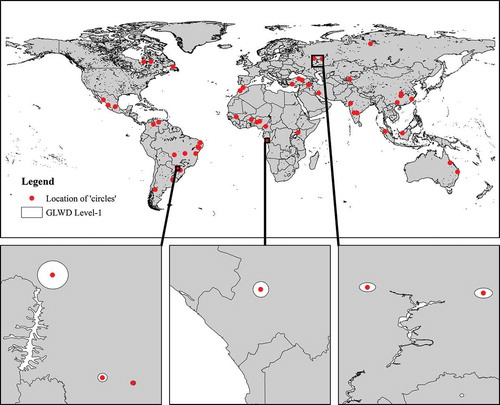
On investigating the database it became apparent that a small number of lakes were represented by a circle of approximate lake size instead of the actual lake outline (examples are shown in Figure 2). These were excluded from further analysis, as whilst it would be possible to produce a map of waterbodies from the water mask algorithm applied here (MacCallum and Merchant 2012), this was not the aim of this exercise and our objective was to use existing lake outline information instead of generating new outlines or correcting errors (although this may be the focus of additional work in the future). As a result of this, 51 waterbodies were excluded reducing the original GLWD Level-1 inventory to 3670 waterbodies. Additionally, using information on the location of dams and reservoirs from the Global Reservoir and Dam (GRanD) database (Lehner et al. 2011), the GLWD predetermined status of ‘lake’ or ‘reservoir’ was validated for all waterbodies. As a result, some GLWD ‘lakes’ were assigned a ‘reservoir’ status. Waterbodies that were not lakes or reservoirs, were assigned a new status. The terms ‘lagoon’, ‘coastal bay’, ‘river’, ‘estuary’, ‘fjord’, ‘glacier’ (defined in Section 2), and ‘other’ were used to fulfil this purpose.

Figure 2. Map showing the location of 51 lake outlines identified as ‘circles’ on GLWD Level-1 inventory, including zoom-in windows in three locations.

Finally, almost 60% of the lake names were missing from the original GLWD Level-1 inventory. Even though some of these could have been retrieved from Google^TM Maps, the validity of the toponymy was uncertain and so the original GLWD lake ID numbers were used to avoid confusion due to missing, multiple, or uncertain lake names.

4.2 Selection criteria based on remote sensing

The criteria that satisfy the first objective of the selection protocol selected lakes conforming to (i) minimum detectable lake area filter, (ii) average number of daytime observations per year (‘pixel counts’), and (iii) water mask area compared to total lake surface area (fractional area, F). The automated facilities provided by ESA’s ATSR Reprocessing for Climate Lake Surface Water Temperature (ARC-Lake) project were used to apply these three remote-sensing filters to ATSR2/AATSR archive data (cf. MacCallum and Merchant 2013). A description of these three selection criteria is presented below.

4.2.1 5 × 5 water cell filter

A minimum size spatial filter was applied to the image data to exclude waterbodies that were too small or irregular for reliable detection and mapping with remote-sensing mapping and thus having the highest likelihood of land contaminating pixels assumed to be water (resulting from geo-location inaccuracies). The filter consisted of a 5 × 5 pixel (equating to approximately 5 km × 5 km) kernel and was developed as part of the ARC-Lake water detection scheme (MacCallum and Merchant 2013).

The ARC-Lake water detection scheme combines GLWD polygons and a binary land/water mask and was applied to the full ATSR2/AATSR time period (1995–2012), recording counts of positive water detection on a 1/120° grid for the entire period. The scheme was designed to overcome limitations arising from inaccuracies in GLWD polygons due to (a) mapping issues and (b) the representation of target areas for a single moment in time, which might not capture seasonal or long-term variability in surface area. Using the GLWD polygons as a basis for target location, but not limited by, a filter based on counts of positive water detection was applied on a target-by-target basis to reduce potential land contamination from mixed land/water pixels. Subsequently, a further image filter was applied to exclude targets where the largest individual area of water was smaller than a 5 × 5 area of contiguous water cells on the 1/120° grid.

4.2.2 Pixel count

To determine an estimate of the likely number of remotely sensed observations that could be expected from a lake in any one year (or period of years), results from the ARC-Lake water detection scheme were analysed across the complete ATSR2/AATSR archive (1995–2012). The automated water detection algorithm returned the number of daytime, clear-sky, and ice-free observations of water (within lake) over the 18-year period, for each 1/120° grid cell (‘pixel counts’). This number is influenced by seasonal ice and cloud cover, and by changes in lake surface area. Larger values increase the likelihood that temporal coverage of image data in the archive is sufficient to estimate trends in satellite-retrieved physical parameters. Considering the maximum value of pixel counts across each potential target, a threshold of 10 pixel counts per year was used. This meant that only lakes with at least 10 daytime observations in at least one water cell per waterbody per year were retained on the candidate list. Due to cloud contamination, the maximum daytime observations per year in any one waterbody in this data set was 42 (Figure 3). The pixel count threshold was used to ensure that the selected lakes are likely to provide frequent enough observations (i.e. at least monthly, depending on cloud cover) to allow the study of seasonal patterns and lake phenology; an important aspect of long-term environmental change studies. However, whilst we have assumed a minimum of 10 observations per year, this value requires further critical analysis, including whether key lake phenology events can be adequately captured, and is the subject of ongoing work. Clearly though, for other applications that operate at different temporal scales the selection of this minimum number of observations will be critical in determining the viability and utility of a remote-sensing-based approach.

Figure 3. Frequency of pixel counts per lake per year.

4.2.3 Fractional area

Based on the pixel count data, a binary land/water mask representing the maximum water extent for each target over the entire 1995–2012 time period was generated for each waterbody on the list. Using this information, the ratio, F, of the water mask area to the total surface area of the waterbodies under investigation was calculated (called ‘fractional area’ hereon) to investigate what percentage of the lake surface area could repeatedly be remotely sensed using daytime satellite (ATSR2/AATSR) observations. A threshold of 30% was set as a minimum ratio for this criterion, meaning that at least 1/3 of the lake should be remotely sensed over the 1995–2012 period. This threshold ensures that a large enough area of the lake is monitored through the years, accounting for bias that can arise from extracting data from only small parts of a lake, particularly when sub-basins with potentially distinct ecological characters exist in a single lake.

This three-step filtering process identified a subset of the GLWD Level-1 inventory, which we have called ‘Preliminary Sample’ from here onwards.

4.3 Selection criteria based on lake landscape context

In order to fulfil the second objective of this work, which was to maximize the sample of lake types and behaviours from across the global continuum, a hierarchy of geographical, landscape setting, and lake morphology attributes were considered (cf. WFD 2000; Soranno et al. 2009). Specifically, lakes were selected based upon two criteria: (i) waterbody type and (ii) lake-catchment relationships, whilst (iii) shoreline irregularity, (iv) eco-location, and (v) basin morphometry classes were used to test the degree of representativeness of each class. Seasonality and lake water quality were also considered as selection criteria, but this was hampered by a complete lack of this type of information at a global standardized scale. Nevertheless, the process was designed to include lakes with highly variable surface area (e.g. Aral Sea) and no restrictions were placed on surface area variability, resulting in the inclusion of targets with large seasonal or long-term variations in surface area (e.g. Lake Balqash, Kazakhstan, and the Great Salt Lake, USA; see Supplementary Material for entire list of ephemeral sites). What is more, the variable landscape setting of the candidate waterbodies acts as an indication of expected variability in the ecological characteristics of these sites, and particularly their pH, alkalinity, eutrophication status, and mixing regime.

4.3.1 Waterbody type

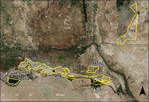
The GloboLakes project will focus on inland lentic waters that have no (or very limited) connection to and interaction with the ocean. As a result, natural fresh and saline lakes, reservoirs, and coastal lagoons were included, whilst rivers, estuaries, fjords, glaciers, and coastal bays were excluded. All waterbodies that appeared to be dry or semi-dry, or had a basin that could not be visually distinguished on Google^TM Earth, were flagged as ephemeral. An example is shown in Figure 4. Potentially ephemeral lakes were also identified by their location in arid areas of the world. Finally, all coastal lagoons in the preliminary sample were identified and classified according to Kjerfve’s (1986) geomorphic classification. Only choked lagoons or those unconnected to the ocean, which have waterbody characteristics dominated by terrestrial inflows and mixing/stratification behaviours consistent with inland freshwater lakes, were included in this study. In total, 71 estuaries, rivers, fjords, glaciers/ice, and coastal bays were identified and removed. A total of 132 lagoons were identified, 22 of which were discarded as belonging to the ‘restricted’ or ‘leaky’ type. The remaining 110 ‘unconnected’ or ‘choked’ lagoons were retained for further consideration.

Figure 4. Examples of cases that were flagged as ephemeral, because they appeared to be dry or semi-dry (Lake ID408), or had a basin that could not be visually distinguished on Google^TM Earth (Lakes ID799 and ID3575).

4.3.2 Lake–catchment relationships

The relationship of a lake to its catchment is a key factor influencing to a lesser or greater extent the physical, chemical, and biological attributes of the waterbody due to its natural role in runoff, sediment and nutrient supply, and susceptibility to human-induced pressures (including indirect effects of climate change) arising from land-use change, water resource management, and biodiversity impacts (Schindler 2009). The GloboLakes study site selection therefore incorporated lakes with a wide range of catchment-to-lake-surface-area ratios.

However, in the case of lagoons, only large catchment areas were selected to ensure that the surrounding land is responsible for the majority of the ecological processes affecting the lagoon and that the effect of the adjacent coastal waters is limited. This only applied to lagoons that are connected to the sea, so for this step all unconnected lagoons remained on the list despite the size of their catchment. A threshold of 10 was used for the catchment-to-lagoon-area ratio (R) resulting in the exclusion of 65% of the preliminary sample choked lagoons that are connected (whether permanently or not) to the sea.

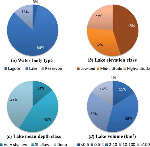
By applying these two criteria to the data, the preliminary sample was further reduced to 961 waterbodies. The Caspian Sea, with a surface area equal of 378,119 km², was removed as an excessively large outlier, which is generally treated as sea in most global remote sensing and modelling systems. The remaining 960 waterbodies (which include 805 lakes, 122 reservoirs, and 33 lagoons, including 41 ephemeral sites as identified in this study; Figure 5(a)) will be referred to ‘GloboLakes sites’ from here onwards; a complete list of these lakes with their names, coordinates, country, and waterbody type is provided in the supplementary material.

Figure 5. Pie charts showing relative percentages (%) of GloboLakes sites based on: (a) waterbody type, (b) lake elevation, (c) lake mean depth (where available), and (d) lake volume (where available).

4.4. Representativeness of selected lakes

The resulting GloboLakes sites were analysed using the three criteria described below to assess how well each criterion-relevant class is represented in the sample.

4.4.1 Shoreline irregularity

The Shore Development Index (SDI) was used as a measure of shoreline irregularity and is the ratio of the shore length (perimeter of lake), L, to the length of the circumference of a circle of area equal to that of the lake, A, (Hutchinson 1957):

(1)

The SDI is dimensionless and generally ranges between 1 (perfectly circular lakes) and 10 (highly irregular lakes), with values over 10 being less common (Håkanson 2004). As there is no known published classification of the regularity of lakes according to their shoreline development index, in this study we used the classes shown below:

• - Circles; SDI = 1

• - Circular; 1 < SDI ≤ 3

• - Regular; 3 < SDI ≤ 5

• - Irregular; 5 < SDI ≤ 8

• - Highly irregular; SDI > 8

The SDI scores for all GloboLakes sites were calculated using Equation (1). Most GloboLakes sites (91.1%) have circular to regular shorelines, an optimum shape from a remote-sensing perspective, whilst only 84 sites are irregular or highly irregular. Investigation of the data showed no correlation between high SDI scores and low pixel count values (linear R² = 0.0021, where R² is the coefficient of determination). Lower pixel counts were mostly observed at high latitudes, where the periods of lake ice cover last for longer, whilst the SDI depends on the lake origin and landscape, with high SDI scores most common amongst reservoirs. As a result, the pixel count filter used in this study did not seem to impose bias on the SDI distributions of the GloboLakes sites.

4.4.2 Eco-location

Ideally, the GloboLakes study lakes should seek to represent the widest possible geographical distribution, with lakes included from all biomes and climatic zones in the world. The ecoregion of each lake, along with topographic information (altitude) and geographical location (latitude), was used to classify lakes according to their ‘eco-location’. The Terrestrial Ecoregions of the World (TEOW) database (Olson et al. 2001) was used to identify different terrestrial ecoregions and ensure all (or the majority) are represented. With the exception of ‘Rock and Ice’, all TEOWs are represented by the GloboLakes sites (Figure 6). In the GLWD Level-1 database, only three lakes are situated within this ecoregion, two of which were identified as glaciers in this work (and consequently discarded) and the third was filtered out during the remote-sensing-based selection process. ‘Boreal, Taiga’ and ‘Tundra’ are by comparison under-represented in the GloboLakes sites due to these lakes being subject to long freezing periods and frequent cloud cover (and subsequently low pixel counts). By contrast, montane and temperate grasslands seem to be generously represented in the GloboLakes sites. This is probably because most GLWD Level-1 waterbodies located within ‘montane grasslands’ (97%) and ‘temperate grasslands’ (90%) are lakes with circular to regular shorelines (1 < SDI ≤ 5) and thus easily detectable with remote sensing, which increased their chances of being selected in this study.

Figure 6. Map showing the spatial distribution of the GloboLakes sites globally, based on the Terrestrial Ecoregions of the World (TEOW) (Olson et al. 2001), lake surface area (variable circle diameter) and Shoreline Development Index (SDI) regularity class (in different shades of blue).

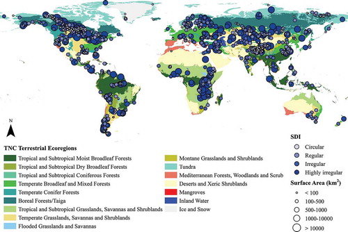
Between the Southern and Northern Hemispheres, the latitudinal distribution of the GloboLakes sites is asymmetrical, with the vast majority (>85%) found in the Northern Hemisphere and most of them above 30°N. There are no GLWD Level-1 lakes (and in extension GloboLakes sites) situated below 60°S (Figure 6), that is, Antarctica. Compared with GLWD Level-1 inventory, there seem to be relatively few high northern latitude lakes (60°–90°N) in the GloboLakes sites due to issues of frequent cloud and long ice cover, which contrasts with the presence of relatively more waterbodies in the latitude band 30°–60°N, when compared to the GLWD Level-1 distribution.

According to the European Union (EU) Water Framework Directive typology for altitude, lowland lakes lie below 200 m, mid-altitude lakes lie between 200, and 800 m and high-altitude lakes lie above 800 m (WFD 2000). Almost half of the GloboLakes sites are lowland (45%), one-third (32%) are mid-altitude, and the rest (23%) are high-altitude waterbodies (Figure 5(b)). Of the 432 lowland waterbodies, 30 are situated below 0 m and 34 at 0 m. Compared with the GLWD Level-1 inventory, the GloboLakes sites contain relatively fewer mid-altitude and more high-altitude lakes. Investigation showed that 57% of the mid-altitude lakes that were discarded during the selection process, are smaller than 100 km², which limits their detectability with remote sensing, whilst 12% of the larger (≥100 km²) ones are situated at high latitudes (north of 60°N), which reduces their average pixel count per year due to long freezing periods and frequent cloud cover. On the other hand, high-altitude lakes generally exhibit circular to regular shorelines (94% of total high-altitude GLWD Level-1 waterbodies), which increases their detectability with remote sensing.

4.4.3 Basin morphometry

The candidate list of lakes should ideally include lakes with variable morphological characteristics, incorporating relatively small to medium-sized lakes and some of the largest lakes in the world in terms of surface area and volume, as well as shallow and deep lakes. The GLWD Level-1 inventory lists the largest 3721 lakes and reservoirs in the world, including lakes with surface area greater than 50 km² and reservoirs with storage capacity greater than 0.5 km³. According to the Annex A of the EU Water Framework Directive (WFD 2000) lake typology for surface area, all GLWD Level-1 waterbodies are classified as large (>0.5 km²). The GloboLakes sites contain relatively few lakes with surface area less than 100 km² and more towards the middle and upper end of the size classes. The latter reflects the limitations of currently available remote-sensing systems with respect to monitoring (relatively) small lakes, especially when their shape is irregular.

According to the EU WFD typology for depth, very shallow lakes have a mean depth of less than 3 m, shallow lakes between 3 and 15 m and deep lakes have a mean depth greater than 15 m (WFD 2000). There are no data for mean depth in the GLWD database, but for 151 waterbodies the information was derived from an extensive literature research and from existing online databases. Figure 5(c) shows that of the GloboLakes sites with known mean depths, most are either classified as shallow (45%) or deep (41%). Similarly, information on volume was unavailable for most of the GLWD Level-1 waterbodies (82%) and GloboLakes sites (78%). However, the 205 lakes for which volume data were available, or were found in the literature or online, cover the entire continuum with the majority (68%) being between 2 and 100 km³ (Figure 5(d)).

5. Discussion and conclusions

The aim of this work was to use a combination of remote-sensing techniques and lake typology criteria in order to select a list of globally distributed lakes and reservoirs that (a) are appropriate for an environmental change study based on remote-sensing data and (b) span a wide range of lake characteristics. The long archive of ATSR2 and AATSR sensors (1995–2012) on-board two European Space Agency satellites and a comprehensive lake database that lists the largest lakes and reservoirs in the world were utilized for this purpose. The methodology proposed here combined spatial filters of remotely sensed detectable area of lake water accounting for land and cloud contamination, and number of daytime satellite observations per year. In addition, auxiliary information sourced in GLWD and other online databases helped inform the site selection with the use of a number of typology criteria, including lake and catchment morphological data and ecological setting. A total of 960 lakes, lagoons, and reservoirs were selected using this process with surface areas between 48,000 and 82,000 km² and spanning a wide range of ecological characteristics fulfilling the two main aims of this study.

Uncertainty related to the GLWD data meant that some of the available information was used with caution in this work. For example, the GLWD polygons only represent the target area for a single moment in time, and therefore do not capture seasonal or long-term changes in surface area and may not even provide an accurate representation of the lake area for any time in the ATSR2/AATSR observing period. As a result of this, the development of a water detection algorithm for the ATSR2/AATSR archive (MacCallum and Merchant 2012), which could then be used for the site selection, was an essential process for this work. In addition, the GLWD catchment area and altitude estimations were based on a rather coarse data set at 1 km × 1 km spatial resolution, and their associated uncertainty is due to scaling issues and model inaccuracies (Lehner and Döll 2004). Ongoing work within the GloboLakes project aims to address all these issues.

The relative paucity of global standardized lake and catchment data that are currently available was one of the main limitations of this work. The unavailability of lake depth, volume, seasonality, and water quality data for most lakes across the globe, and the unknown reliability of some of the existing data, restricted the application of all selection criteria for the second objective, which was to select waterbodies that span a wide range of ecological behaviours. Based on global data sets, only the eco-location of study sites could be derived with confidence. The GloboLakes project aims to deliver most of this missing information, including modelled lake morphometry (mean, maximum depth, and volume) and lake water quality data.

Even though SDI is a useful measure of lake shoreline irregularity, and can be used as an estimation of effective area of open water available for remotely sensed observations, it should be used with caution. Some of the lakes that were classified as ‘highly irregular’ are the largest lakes (by surface area) of the world, such as the Great Slave Lake, Lake Chad and Lake Nettiling. These three lakes show localized irregularity that results in high SDI scores, but have large enough basins that permit reliable and repeatable remotely sensed observations of a considerable proportion of the lake surface. To overcome problems like these when selecting candidate lakes, the pixel count filtering technique is an essential tool to estimate the effective area of open water available for remotely sensed observations.

The final sample of GloboLakes sites has a high degree of variability in their landscape context as defined by ecoregion setting, landscape position, lake-catchment relation, and, finally, lake morphology. These systems embrace a wide range of formative mechanisms (e.g. volcanic, glacial, tectonic, fluvial, etc.) and feature a spectrum of human pressures – from essentially wilderness settings and natural conditions to intensely developed, highly regulated and modified conditions. Accordingly, they provide a unique testing opportunity to evaluate trends in water quantity, quality, and ecosystem response as a result of changing pressures, and as a direct and indirect consequence of climate change.

Whilst currently constrained by the need to work on systems of a particular size and shape that lend themselves to analysis using the current generation of Earth Observation (EO) tools, the future of global lake analysis with remote sensing looks much brighter as the next generation of platforms (e.g. the Sentinel series of satellite sensors) are launched and commissioned. The new Sentinel satellites will ensure spatially, temporally, and spectrally enhanced data continuity as they build on the success of current and past sensors. For example, the synthetic aperture radar (SAR) system on Sentinel-1 and the SPOT (Satellite Pour l’ Observation de la Terre)- and Landsat-like data from Sentinel-2 will make it possible to track variability in lake area. However, despite improved spatial, spectral, and radiometric resolutions of new missions, the issues highlighted in this work will be important considerations for the application of systematic retrieval of lake water quality from satellite-based observations. In particular, we have shown that lake size, shape, cloudiness, and the availability (or lack of it) of lake contextual information, can inhibit the utility of satellite-based observations, and such considerations will remain for future missions. The methodology proposed here should be of value to all researchers hoping to exploit archive and future satellite-based missions for lake studies. In particular, it will be applicable to the Sea and Land Surface Temperature Radiometer (SLSTR), which will be the successor to the (A)ATSR, while the size and shape of the lakes selected will be appropriate for use with OLCI data; both of which are carried on-board Sentinel-3 that was launched in February 2016. Based on these improved satellite sensor technologies, future application of the proposed site selection protocol will enable the selection of much smaller lakes than possible before. In addition, the use of such datasets will be further enhanced with new data-handling and sharing protocols providing unprecedented interoperability. In particular, the ESA Copernicus Programme (http://www.copernicus.eu/) provides free data access and the EU Infrastructure for Spatial Information in the European Community (INSPIRE) directive (http://inspire.ec.europa.eu/) aims to improve the availability, quality, accessibility, and sharing of data across Europe. All of this points to a significant potential of remote sensing for regional to global limnological analysis but key questions still remain to be resolved. The most important of these is that of whether sufficient observations exist to allow retrieval of lake phenology. We have assumed that a minimum of 10 observations per year will allow this, but this requires further analysis, which we are currently undertaking, and will be a key output of the GloboLakes project.

Acknowledgments

This work was supported by the United Kingdom Natural Environment Research Council (NERC) under Grant NE/J024279/1. The authors would like to thank University of Edinburgh and the ARC-Lake project for access to data, and acknowledge our partners in the GloboLakes Consortium, namely Universities of Stirling, Reading and Glasgow, Plymouth Marine Laboratory (PML) and the Centre for Ecology and Hydrology (CEH).

Disclosure statement

No potential conflict of interest was reported by the authors.

Supplemental data

Supplemental data for this article can be accessed here.

Additional information

Funding

This work was supported by the United Kingdom Natural Environment Research Council [Grant number NE/J024279/1].

References

- Adrian, R., C. M. O’Reilly, H. Zagarese, S. B. Baines, D. O. Hessen, W. Keller, D. M. Livingstone, et al. 2009. “Lakes as Sentinels of Climate Change.” Limnology and Oceanography 54: 2283–2297. doi:10.4319/lo.2009.54.6_part_2.2283.
- Arhonditsis, G. B., M. T. Brett, C. L. DeGasperi, and D. E. Schindler. 2004. “Effects of Climatic Variability on the Thermal Properties of Lake Washington.” Limnology and Oceanography 49: 256–270. doi:10.4319/lo.2004.49.1.0256.
- Blenckner, T., R. Adrian, D. M. Livingstone, E. Jennings, G. A. Weyhenmeyer, D. G. George, T. Jankowski, et al. 2007. “Large-Scale Climatic Signatures in Lakes across Europe: A Meta-Analysis.” Global Change Biology 13: 1314–1326. doi:10.1111/gcb.2007.13.issue-7.
- ESA (European Space Agency). “ArcLake (ATSR Reprocessing for Climate: Lake Surface Water Temperature & Ice Cover) project 2016.” Accessed February 16 2016. http://www.geos.ed.ac.uk/arclake
- EUROPA (European Commission) WFD (Water Framework Directive). 2011. Accessed February 18 2016. http://ec.europa.eu/environment/water/water-framework/index_en.html
- Gerten, D., and R. Adrian. 2000. “Climate-Driven Changes in Spring Plankton Dynamics and the Sensitivity of Shallow Polymictic Lakes to the North Atlantic Oscillation.” Limnology and Oceanography 45: 1058–1066. doi:10.4319/lo.2000.45.5.1058.
- Golosov, S., A. Terzhevik, I. Zverev, G. Kirillin, and C. Engelhardt. 2012. “Climate Change Impact on Thermal and Oxygen Regime of Shallow Lakes.” Tellus A 64: 17264. doi:10.3402/tellusa.v64i0.17264.
- Håkanson, L. 2004. Lakes: Form and Function. Caldwell, NJ: The Blackburn Press.
- Hardy, J. T. 2003. Climate Change: Causes, Effects and Solutions. Chichester: Wiley.
- Herdendorf, C. E. 1982. “Large Lakes of the World.” Journal of Great Lakes Research 8: 379–412. doi:10.1016/S0380-1330(82)71982-3.
- Hutchinson, G. E. 1957. A Treatise on Limnology; Volume 1: Geography, Physics and Chemistry. New York: John Wiley and Sons editions.
- Jones, J., and M. T. Brett. 2014. “Lake Nutrients, Eutrophication, and Climate Change.” In Global Environmental Change, edited by B. Freedman. Dordrecht: Springer. doi:10.1007/978-94-007-5784-4_109.
- Kjerfve, B. 1986. “Comparative Oceanography of Coastal Lagoons.” In Estuarine Variability, edited by D. A. Wolfe. London: Academic.
- Latifovic, R., and D. Pouliot. 2007. “Analysis of Climate Change Impacts on Lake Ice Phenology in Canada Using the Historical Satellite Data Record.” Remote Sensing of Environment 106: 492–507. doi:10.1016/j.rse.2006.09.015.
- Lehner, B., and P. Döll. 2004. “Development and Validation of a Global Database of Lakes, Reservoirs and Wetlands.” Journal of Hydrology 296: 1–22. doi:10.1016/j.jhydrol.2004.03.028.
- Lehner, B., C. R. Liermann, C. Revenga, C. Vörösmarty, B. Fekete, P. Crouzet, P. Döll, et al. 2011. Global Reservoir and Dam (Grand) Database. Technical Documentation, Version 1.1. Global Water System Project (GWSP), Montreal.
- Livingstone, D. M., and M. Dokulil. 2001. “Eighty Years of Spatially Coherent Austrian Lake Surface Temperatures and Their Relationship to Regional Air Temperature and the North Atlantic Oscillation.” Limnology and Oceanography 46: 1220–1227. doi:10.4319/lo.2001.46.5.1220.
- MacCallum, S. N., and C. J. Merchant. 2012. “Surface Water Temperature Observations of Large Lakes by Optimal Estimation.” Canadian Journal of Remote Sensing 38: 25–45. doi:10.5589/m12-010.
- MacCallum, S. N., and C. J. Merchant. 2013. ARC-Lake – Algorithm Theoretical Basis Document v1.3. Edinburgh: The University of Edinburgh.
- Mahowald, N. M., R. G. Bryant, J. Del Corral, and L. Steinberger. 2003. “Ephemeral Lakes and Desert Dust Sources.” Geophysical Research Letters 30: 1074. doi:10.1029/2002GL016041.
- Nixon, S., J. Grath, and J. Bøgestrand. 1998. “The European Environment Agency’s Monitoring and Information Network for Inland Water Resources.” Technical Guidelines for Implementation, Technical Report No. 7. Copenhagen: EUROWATERNET, European Environment Agency.
- NOAA (National Oceanic and Atmospheric Administration) NS&T (National Status and Trends programme). 2016. Accessed February 18, 2016. http://products.coastalscience.noaa.gov/collections/ltmonitoring/nsandt/
- Olson, D. M., E. Dinerstein, E. D. Wikramanayake, N. D. Burgess, G. V. N. Powell, E. C. Underwood, J. A. D’Amico, et al. 2001. “Terrestrial Ecoregions of the World: A New Map of Life on Earth.” Bioscience 51: 933–938. doi:10.1641/0006-3568(2001)051[0933:TEOTWA]2.0.CO;2.
- Palmer, S., P. Hunter, T. Lankester, S. Hubbard, E. Spyrakos, A. Tyler, M. Presing, et al. 2015a. “Validation of Envisat MERIS Algorithms for Chlorophyll Retrieval in a Large, Turbid and Optically-Complex Shallow Lake.” Remote Sensing of Environment 157: 158–169. doi:10.1016/j.rse.2014.07.024.
- Palmer, S. C. J., D. Odermatt, P. D. Hunter, C. Brockmann, M. Présing, H. Balzter, and V. R. Tóth. 2015b. “Satellite Remote Sensing of Phytoplankton Phenology in Lake Balaton Using 10 Years of MERIS Observations.” Remote Sensing of Environment 158: 441–452. doi:10.1016/j.rse.2014.11.021.
- Politi, E., M. E. J. Cutler, and J. S. Rowan. 2012. “Using the NOAA Advanced Very High Resolution Radiometer to Characterise Temporal and Spatial Trends in Water Temperature of Large European Lakes.” Remote Sensing of Environment 126: 1–11. doi:10.1016/j.rse.2012.08.004.
- Politi, E., M. E. J. Cutler, and J. S. Rowan. 2016. “Assessing the Utility of Geospatial Technologies to Investigate Environmental Change within Lake Systems.” Science of the Total Environment 543: 791–806. doi:10.1016/j.scitotenv.2015.09.136.
- Rashki, A., D. G. Kaskaoutis, A. S. Goudie, and R. A. Kahn. 2013. “Dryness of Ephemeral Lakes and Consequences for Dust Activity: The Case of the Hamoun Drainage Basin, Southeastern Iran.” Science of the Total Environment 463-464: 552–564. doi:10.1016/j.scitotenv.2013.06.045.
- Read, J. S., L. A. Winslow, G. J. A. Hansen, J. Van Den Hoek, P. C. Hanson, L. C. Bruce, and C. D. Markfort. 2014. “Simulating 2368 Temperate Lakes Reveals Weak Coherence in Stratification Phenology.” Ecological Modelling 291: 142–150. doi:10.1016/j.ecolmodel.2014.07.029.
- Schindler, D. W. 2009. “Lakes as Sentinels and Integrators for the Effects of Climate Change on Watersheds, Airsheds, and Landscapes.” Limnology and Oceanography 54: 2349–2358. doi:10.4319/lo.2009.54.6_part_2.2349.
- Soranno, P. A., K. E. Webster, K. S. Cheruvelil, and M. T. Bremigan. 2009. “The Lake Landscape-Context Framework: Linking Aquatic Connections, Terrestrial Features and Human Effects at Multiple Spatial Scales.” Verhandlungen des Internationalen Verein Limnologie 30: 695–700.
- Stevens, D. L. Jr. 1994. “Implementation of a National Monitoring Program.” Journal of Environmental Management 42: 1–29. doi:10.1006/jema.1994.1057.
- UNEP (United Nations Environment Programme). 2000. “Lakes and Reservoirs: Similarities, Differences and Importance.” UNEP International Environmental Technology Centre (IETC) Short Report 1, Japan.
- US EPA (Environmental Protection Agency) EMAP (Environmental Monitoring & Assessment Program). 2016. Accessed February 18 2016 https://archive.epa.gov/emap/archive-emap/web/html/index.html
- USFS (US Forest Service) FIA (Forest Inventory and Analysis) programme. 2016. Accessed February 18 2016. http://www.fia.fs.fed.us/
- USGS (US Geological Survey) NAWQA (National Water-Quality Assessment programme). 2016. Accessed February 18 2016. http://water.usgs.gov/nawqa/
- Verpoorter, C., T. Kutser, D. A. Seekell, and L. J. Travnik. 2014. “A Global Inventory of Lakes Based on High-Resolution Satellite Imagery.” Geophysical Research Letters 41: 6396–6402. doi:10.1002/2014GL060641.
- Vincent, W. F. 2009. “Effects of Climate Change on Lakes.” In Encyclopedia of Inland Waters Vol. 3, edited by G. E. Likens, 55–60. Elsevier: Oxford.
- Weyhenmeyer, G. A., T. Blenckner, and K. Pettersson. 1999. “Changes of the Plankton Spring Outburst Related to the North Atlantic Oscillation.” Limnology and Oceanography 44: 1788–1792. doi:10.4319/lo.1999.44.7.1788.
- Weyhenmeyer, G. A., R. Adrian, U. Gaedke, D. M. Livingstone, and S. C. Maberly. 2002. “Response of Phytoplankton in European Lakes to a Change in the North Atlantic Oscillation.” Verhandlungen des Internationalen Verein Limnologie 28: 1436–1439.
- WFD (Water Framework Directive). 2000. Directive 2000/60/EC of the European Parliament and of the Council of 23 October 2000 Establishing a Framework for Community Action in the Field of Water Policy, Luxembourg.
- Wilhelm, S., T. Hintze, D. M. Livingstone, and R. Adrian. 2006. “Long-Term Response of Daily Epilimnetic Temperature Extrema to Climate Forcing.” Canadian Journal of Aquatic Science 63: 2467–2477. doi:10.1139/f06-140.
- Williamson, C. E., J. A. Brentrup, J. Zhang, W. H. Renwick, B. R. Hargreaves, L. B. Knoll, E. P. Overholt, and K. C. Rose. 2014. “Lakes as Sensors in the Landscape: Optical Metrics as Scalable Sentinel Responses to Climate Change.” Limnology and Oceanography 59: 840–850. doi:10.4319/lo.2014.59.3.0840.
- Williamson, C. E., J. E. Saros, W. F. Vincent, and J. P. Smol. 2009. “Lakes and Reservoirs as Sentinels, Integrators, and Regulators of Climate Change.” Limnology and Oceanography 54: 2273–2282. doi:10.4319/lo.2009.54.6_part_2.2273.