Towards a set of agrosystem-specific cropland mapping methods to address the global cropland diversity

ABSTRACT

Accurate cropland information is of paramount importance for crop monitoring. This study compares five existing cropland mapping methodologies over five contrasting Joint Experiment for Crop Assessment and Monitoring (JECAM) sites of medium to large average field size using the time series of 7-day 250 m Moderate Resolution Imaging Spectroradiometer (MODIS) mean composites (red and near-infrared channels). Different strategies were devised to assess the accuracy of the classification methods: confusion matrices and derived accuracy indicators with and without equalizing class proportions, assessing the pairwise difference error rates and accounting for the spatial resolution bias. The robustness of the accuracy with respect to a reduction of the quantity of calibration data available was also assessed by a bootstrap approach in which the amount of training data was systematically reduced. Methods reached overall accuracies ranging from 85% to 95%, which demonstrates the ability of 250 m imagery to resolve fields down to 20 ha. Despite significantly different error rates, the site effect was found to persistently dominate the method effect. This was confirmed even after removing the share of the classification due to the spatial resolution of the satellite data (from 10% to 30%). This underlines the effect of other agrosystems characteristics such as cloudiness, crop diversity, and calendar on the ability to perform accurately. All methods have potential for large area cropland mapping as they provided accurate results with 20% of the calibration data, e.g. 2% of the study area in Ukraine. To better address the global cropland diversity, results advocate movement towards a set of cropland classification methods that could be applied regionally according to their respective performance in specific landscapes.

1. Introduction

Covering about 12% of the Earth’s land surface, cropland experienced tremendous expansion in area and uneven geographical reallocation in the past decade (Foley et al. 2011). Agricultural lands are changing continuously and intensively under the context of global warming and anthropogenic transformation. When addressing food security, accurate mapping of cropland at both global and local scales is crucial for the scientific community, governments and non-government agencies, farmers, and other stakeholders (Olofsson et al. 2012; Pflugmacher et al. 2011; Fritz and See 2008; Giri et al. 2013; Wu et al. 2014; Husak et al. 2008; Thenkabail and Wu 2012). In many food-insecure regions, understanding and characterizing agricultural production remain a major challenge (Fritz, See, and Rembold 2010). The location and extent of agricultural lands are used as baseline information for crop production monitoring, regardless of the scale (Justice and Defourny et al. 2007). Moreover, such crop maps would be particularly helpful in regions where reliable information on agriculture is inconsistent over time due to the limited extent of agricultural surveys or to the insecure access to terrain as a result of political instability or wars (Delrue et al. 2013; Hannerz and Lotsch 2006). Timely delivered crop maps may provide objective information and prove to be a useful tool for decision-making in cropland management and in early warning systems (e.g. Global Information and Early Warning System on Food and Agriculture (GIEWS), Famine Early Warning Systems Network (FEWS-NET)) (Delrue et al. 2013; Hannerz and Lotsch 2006; Vancutsem et al. 2012).

Satellite remote sensing proved to be an important tool for crop mapping (Wu et al. 2008; Barrett 2013; Gallego et al. 2014) as it allows to map the cropland area and crop distribution across scales. Since the launch of Landsat-1, satellite imagery has been included in crop inventory (Allen 1990; Battese, Harter, and Fuller 1988). Since then, a large variety of methods for mapping cropland and its changes have been devised (Alcantara et al. 2012; Estel et al. 2015). Nowadays, the Cropland Data Layer (CDL) – a 30 m annual crop-specific crop-type map based on decision tree, ground truth, and other ancillary data, such as the National Land Cover Data set (Boryan et al. 2011) – produced by the National Agricultural Statistics Service (NASS) of the US Department of Agriculture (USDA), counts amongst the most advanced operational satellite-based crop inventory programmes. Other methods found in the literature include unsupervised approaches (Biradar et al. 2009; Dheeravath et al. 2010; Vintrou et al. 2012a) to supervised methods such as decision trees (Pittman et al. 2010; Shao and Lunetta 2012), Support Vector Machine (Shen et al. 2011; Shao and Lunetta 2012; Lambert, Waldner, and Defourny 2016), Random Forest (Watts et al. 2009; Müller et al. 2015), neural networks (Kussul et al. 2015; Skakun et al. 2015), data mining (Vintrou et al. 2013), or a combination of hard and soft classifiers (Pan et al. 2012). Considerable attention has also been devoted to optimizing the selection of the dates (Murakami et al. 2001; Van Niel and McVicar 2004; Löw et al. 2013; Conrad et al. 2014) used for the classification or to derive adequate temporal features (Xiao et al. 2005; Arvor et al. 2012; Zhong, Gong, and Biging 2014; Müller et al. 2015; Waldner, Canto, and Defourny 2015; Matton et al. 2015). Studies such as those of Foerster et al. (2012) and Conrad et al. (2010) found that the crop calendar was especially helpful for crop mapping. Also, the selection of a pixel-based or object-based approach influences both the performance of classifiers and the quality of crop maps (Conrad et al. 2011; Peña-Barragán et al. 2011; Matton et al. 2015). Efficient annual cropland mapping approaches for operational crop monitoring must comply with several requirements such as timeliness, accuracy, a high degree of automation, and cost-effectiveness (Waldner et al. 2015b). Those requirements constrain the range of the usable approaches.

Another important factor that affects the accuracy of crop maps is the spatial resolution of the imagery. In fact, the spatial resolution itself can be a source of bias in classification (Boschetti, Flasse, and Brivio 2004) as well as in area estimation (Ozdogan and Woodcock 2006; Soares, Galvão, and Formaggio 2008). The importance of the bias is directly linked to the spatial fragmentation of the agricultural system of interest and the class definition (Ozdogan and Woodcock 2006; Soares, Galvão, and Formaggio 2008). For instance, Vintrou et al. (2012a) highlighted that the accuracy of MODIS-derived maps of contrasted Malian agrosystems was linearly correlated (coefficient of determination of 0.8) with the fragmentation (defined by the mean patch size index). The net effect is that for the same spatial resolution, some places will exhibit much larger errors than others, depending on landscape spatial structure. Cushnie (1987) investigated the effect of spatial resolution and degree of internal variability within land-cover types on classification accuracies. Classification accuracies within internally homogeneous classes were found to be high at all spatial resolutions from 5 to 20 m. In contrast, classification accuracies of land-cover types characterized by a high degree of internal variability improved by up to 20% as spatial resolution was coarsened because the proportion of scene noise was reduced. Duveiller and Defourny (2010) presented a conceptual framework to define quantitatively the spatial resolution requirements for both crop area estimation and crop growth monitoring based on user-defined constraints. The methodology focused on how fields of specific crops are seen by instruments of different resolving power accounting for the point spread function of the sensor. It relied on the concept of pixel purity, e.g. the degree of homogeneity of a pixel with respect to the target crop. In the domain of crop classification, Löw and Duveiller (2014) investigated the question of determining the optimal pixel size as finding the coarsest acceptable pixel sizes. Building upon Duveiller and Defourny (2010), the authors defined three criteria (sample size, classification uncertainty, and accuracy) to identify the appropriate pixel size and purity. They demonstrate that there is no one-size-fits-all solution to the optimum pixel size problem: it is specific to a given landscape.

To foster method inter-comparisons, the Joint Experiment of Crop Assessment and Monitoring (JECAM) was created by the Group on Earth Observation Global Agriculture Monitoring Community of Practice. Its overarching goal is to reach a convergence of approaches, develop monitoring and reporting protocols and best practices for a variety of global agricultural systems. JECAM enables the global agricultural monitoring community to compare results based on disparate sources of data, using various methods, over a variety of global cropping systems. To that aim, the JECAM network has adopted a shared definition of the cropland that matches the Food and Agriculture Organization’s (FAO) Land Cover Meta Language. The general definition of annual cropland (including area affected by crop failure) could be as follows: the annual cropland is a piece of arable land that is sowed or planted at least once within a 12-month period. In the context of global mapping, the identification and the validation of the cropland class is limited by the resolutions of the remote-sensing imagery. A specific definition is then proposed: the annual cropland from a remote-sensing perspective is a piece of land of minimum 0.25 ha (minimum width of 30 m) that is sowed/planted and harvestable at least once within the 12 months after the sowing/planting date. The annual cropland produces an herbaceous cover and is sometimes combined with some tree or woody vegetation. There are three known exceptions to this definition. The first concerns the sugarcane plantation and cassava crop, which are included in the cropland class although they have a longer vegetation cycle and are not yearly planted. Second, taken individually, small plots such as legumes do not meet the minimum size criteria of the cropland definition. However, when considered as a continuous heterogeneous field, they should be included in the cropland. The third case is the greenhouse crops that cannot be monitored by remote sensing and are thus excluded from the definition.

As there is a compelling need for accurate cropland maps, the overarching objective is to compare the accuracy of cropland mapping methodologies and test their genericity across the globe. This experiment involves five JECAM sites located in Russia, Ukraine, Argentina, China, and Brazil. Those sites present contrasting growing conditions and characteristics, yet they all have a medium to large average field size. Over time, different classification methods have emerged according to the peculiarities of each cropping system by their respective research teams. Throughout this article, classification methodology encompasses both the satellite data preparation (indices, temporal features) and the classification algorithm itself. To isolate the effect of the methodology, input satellite data were the same for different test sites, and methodologies proposed by the different teams were evaluated on the same calibration and validation data for particular test sites. In order to support the global mapping efforts, this research specifically aims at:

1. evaluating the performance of the classification methods in order to identify their strengths and limitations across a variety of landscapes as well as to evaluate their genericity;

2. quantifying the share of error due to the method itself and the spatial resolution of the data used;

3. assessing the robustness of the methodologies in various agrosystems as an indicator of the potential for upscaling to larger scales with a focus on the spatial or temporal resolutions.

Finally, recommendations for future classification method benchmarking and comparison are also expected to be highlighted.

2. Materials

2.1. Study sites

This study considers five test sites with medium to large average field size but contrasted crop diversities, management practices, and crop calendars. Two of them are located in South America (Brazil and Argentina), while the remaining three are located in Asia and Europe (China, Russia, and Ukraine) (Figure 1(a)).

Figure 1. Location of the JECAM sites and illustration of their diversity with false colour composites (near-infrared, red, green). (a) The red dots locate the five sites overlaid over the Unified Cropland Layer (Waldner et al. 2016) in green. Representative zooms of Landsat-8 false colour composites (near-infrared, red, green) in (b) Argentina, (c) Brazil, (d) China, (e) Russia, and (f) Ukraine.

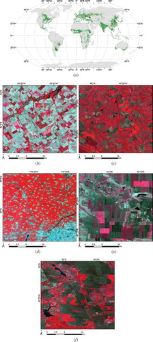
The Argentinian site (100 by 90 km) is located in the Rolling Pampas, a sub-region of the Pampas with gentle slopes (lower than 3%) and rivers (Figure 1(b)). Soils are mostly mollisols with a deep surface layer of high organic matter content. The climate is humid temperate with a homogeneous precipitation regime and an annual mean of about 1000 mm. The dominant crops are soya bean, maize, and wheat (Figure 2). Wheat can be planted as early as June and until the end of July and August. The heading occurs in mid-October, and its harvest occurs at the beginning of December. Wheat can be followed by a so-called late soya bean (sown in December and harvested in April) which would thus result in double cropping systems. Early soya bean and maize are mostly planted as a single-season crop. In these cases, soya bean is planted in November and harvested in March/April whereas maize planted in October and harvested in March. Late maize crops can be planted in December after a fallow or after a winter crop. Agriculture is developed under no-till systems (only a reduced till is done together with planting leaving crop residues over soil surface) and mostly without irrigation. Typical field size is 20 ha but there is a high variability in plot size. Non-cropland areas are mostly for forage including pastures and grasslands.

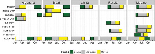
Figure 2. Calendars for the dominant crop types of the five study sites (source: FAO/Global Information and Early Warning System on Food and Agriculture). Considered crops are maize, soya bean, spring barley (s. barley), sugar beet, sunflower, spring cereals (s. cereals), and winter wheat (w. wheat).

In Brazil, the site (80 km by 95 km) is located in the state of São Paulo close to the city of Itatinga (Figure 1(c)). Soils are mainly deep Ferralsols in the area, with local variations of clay content. The climate is humid tropical with a mean temperature of 19°C and precipitations of 1390 mm measured in the past 20 years at the nearby Itatinga Experimental Station of the University of São Paulo. Temperatures and precipitations are lower from June to September, with temperature below 5°C several days each year. The land cover is dominated by cropland, pastures, planted and natural forests, and waterbodies. Annual crops are dominated by soya bean and maize, with two cultivation cycles per year in monoculture or successions (Figure 2). Some of the fields are irrigated with pivot. Sugarcane, which is perennial but has an annual harvesting cycle, is also largely planted in this area. The first harvest of sugarcane occurs around 18 months after plantation, and after that the harvest is annual and occurs mainly between September and November. The size of the parcels is generally between 50 and 150 ha. Permanent pastures and grasslands are present on the east of the area. Forest plantations, mainly eucalyptus and pine, also share a large part of the area, and are harvested by clear cuts.

The Chinese site (75 km by 60 km) is located near the city of Yucheng in the northwest province of Shandong (Figure 1(d)). According to the long-term observation data from the Yucheng Integrated Agricultural Experimental Station, the area has a temperate, semi-arid monsoon climate, with mean annual temperature of 13.1°C and precipitations of 582 mm concentrated from late June to September. The land cover is dominated by cropland, forest, and urban areas, with smaller areas of water and grassland. The dominant crop rotation starts typically with winter wheat followed by summer maize (Figure 2). The sowing of winter wheat concentrates in early October and the harvest usually concludes in mid-June the following year. Summer maize is sown in mid-June, right after the harvest of winter wheat, and harvested at the end of September to early October. The annual cycle is then repeated (Meng, Du, and Wu 2013). Tillage practices vary from intensive tillage with very low residue cover to conservation tillage (including no-till) with little disturbance of the residue (Miao, Qiangzi, and Bingfang 2012). Typical field size ranges from 0.2 to 0.8 ha at the site. Overall, the JECAM in Shandong province is representative of North China Plain farming practices.

The Russian JECAM site (60 km by 85 km) is located in the krai of Stavropol (45° 09ʹ N, 42° 08ʹ E), one of the most important agricultural region in Russia (Figure 1(e)). The climate varies from arid continental to humid continental with yearly average temperature up to 10°C and mean annual precipitation of 560 mm. The landscape is dominated by rolling hills with wide floodplains. The terrain is mostly flat with slopes ranging from 0% to 2%; nearly 15% of the territory is hilly with slopes more than 2%. Effects of soil erosion and desertification – typical for the eastern part of the krai – are negligible at the study site. The dominating crops are winter wheat, spring and winter barley, peas, soya bean, sunflower, winter rape, and perennial grasses with a strong winter crop prevalence (Figure 2). The typical field sizes range from 30 to 130 ha. There are four main crop rotation types with several sub-types; changing from 2-years cycle with winter wheat and clean fallow in the arid eastern parts to 8-year cycle including clean fallow, winter wheat, sugar beet, fodder maize, sunflower, spring barley, and grain maize in the central and western parts.

The test site in Ukraine (150 km by 110 km) is located in the region of the Kyiv oblast (50° 0ʹ N and 30° 16ʹ E) (Shelestov et al. 2013; Kussul et al. 2014) (Figure 1(f)). The climate in the region is humid continental with approximately 709 mm of annual precipitations. Landscape is mostly flat terrain with slopes ranging from 0% to 2%; near 10% of the territory is hilly with slopes about 2–5%. Land-cover classes are quite heterogeneous including croplands, forests, grassland, rivers, lakes, and wetlands. Forests and grasslands dominate its northern part, while the central and southern parts are agriculture-intensive areas. The crop calendar is September–July for winter crops, and April–October for spring and summer crops (Figure 2). Dominant crop types include maize (25% of total cropland area in 2013), winter wheat (16%), soya beans (13%), vegetables (10%), sunflower (9%), spring barley (7%), winter rapeseed (4%), and sugar beet (1%). Due to the relatively large number of major crops and other factors, there is no typical simple crop rotation scheme in this region. Most farmers use different crop rotations depending on specialization. Fields in the region are quite large (except family gardens) with a size ranging up to 250 ha.

2.2. In situ data

For each site, land-cover classes were reduced to a binary cropland/non-cropland legend according to the cropland definition (see Section 1). Every data set collected by each JECAM site institution was also randomly divided into a calibration set (50% of the polygons) to train the classifiers and testing set (the remaining 50% of the polygons) for validation purposes (Table 1). This calibration/validation separation was kept for all algorithms and samples were selected in a way so as to ensure no overlap between training and testing sets.

Table 1. Characteristics of the in situ data sets in terms of coverage, number of polygons, and average polygon size.

Site	Area (ha)	Cropland proportion (%)	Area covered by objects (%)	Number of objects	Proportion of cropland objects (%)	Mean cropland object size (ha)	Mean non-cropland object size (ha)
Argentina	774002	60	1.13	348	81.0	27.1	16.5
Brazil	507728	68	3.68	847	36.0	21.3	22.4
China	360802	54	0.46	92	48.9	17.7	18.7
Russia	362487	59	14.57	588	83.7	77.1	154.9
Ukraine	1135346	76	2.21	608	74.0	46.9	25.2

2.2.1. Argentina

From the 1 June 2013 to the 31 May 2014, several on-road surveys were performed to register the land use and the geolocation at several points. Field boundaries were generated later on thanks to very high resolution imagery and assigned to the different classes according to the field observation points. A total of 348 polygons were generated (282 cropland and 66 non-cropland polygons).

2.2.2. Brazil

Land-use land-cover surveys were performed in December 2014 by collecting data along roads that covered the main part of the site area. A land-cover class was assigned to most of the large fields clearly identifiable from the road, and according to JECAM’s nomenclature. A total of 847 field measurements were collected, from which 326 were within the area selected for this study to have the highest diversity in terms of land cover. A total of 13 different land cover has been found in more than three records, at the highest precision level (crop species). When the soil was bare, the previous crop was identified from residuals left inside the field when possible; this crop was considered as the final class. This was done because some bare soil could be found either on cropland or non-cropland land cover. The coordinates of the centre of each field was measured with a global positioning system (GPS) device, and the polygon of the field was obtained later by visual image analysis. Polygons of the field corresponding to each GPS point was delineated on eight Landsat and DEIMOS images acquired between September 2013 and November 2014.

2.2.3. China

Field work was carried out in mid-May and late August 2014. The field surveys were based on RapidEye imagery acquired in June 2012. The crop types of the sampled fields and other land-cover types were recorded using handheld GPS, and the polygon of the corresponding land-cover types were drawn according to very high resolution imagery. Based on the field survey, six classes including winter wheat, cotton, vegetables, tree, fallow land, and non-arable land were identified. Non-arable land areas include residential area, road, and waterbody. The sample points from wheat and maize yield measurement survey were also used to enrich the field samples. Those points were expanded to polygon samples based on the segmentation of a high-resolution satellite image. One Chinese Satellite GaoFen-1 (GF-1) Wide Field Imager (WFI) data was acquired in 26 May 2014 over China site at peak growing stage. WFI data is at 16 m resolution with three visible bands (red, green, and blue) and one short-wave infrared band (Li et al. 2015). Objects were generated by means of a multi-scale segmentation based on a region-growing technique (Benz et al. 2004; Definiens 2009). To improve the performance of the segmentation, the Constrained Spectral Variance Difference (CSVD) and edge penalty were used. With the CSVD, large objects are preserved as integral entities meanwhile small objects can still be effectively delineated (Chen et al. 2015).

2.2.4. Ukraine

Ground surveys were conducted in June 2014 to collect data on crop types and other land-cover classes. Data were collected along roads using mobile devices with built-in GPS. Each land/crop cover observation was associated with a polygon whose vertices were measured in situ.

2.2.5. Russia

Field data collection was fulfilled during the year 2014, when field surveys data as well as farmers’ remotely verified information was aggregated. Each local farm surveyed provided spatial information on field limits and the corresponding crop types within borders of their competence. Exact field boundaries were reconstructed from Landsat images for the year 2014. Crop type information was validated using MODIS seasonal time-series, when objects with suspicious phenology or one different from class majority were separated. These fields preserved cropland class, but crop type information was suspended. There were 495 fields collected within Stavropol krai borders, encompassing 12 main crop types covering more than 90% of krai’s crop sown area. Since only cropland data was accumulated during these surveys, additional efforts were aimed at non-cropland data collection for the benchmarking experiment. Seasonal Landsat data over test area was processed by phenologically based segmentation routine, which provided homogeneous areas, occupied by a single vegetation class. Such segmentation results were compared with TerraNorte RLC map (Bartalev et al. 2011) to select non-cropland class segments. Phenologically stable and sizable segments were manually selected to provide statistical balance between crop and non-cropland class over test area.

2.3. Satellite data

From daily quality controlled reflectance values of Moderate Resolution Imaging Spectroradiometer (MODIS) Terra and Aqua (MOD09Q1, MYD09Q1, MOD09GA, and MYD09GA), 7-day mean composites were produced according to the procedure developed by Vancutsem et al. (2007). The mean compositing reduces the bidirectional reflectance distribution function effects and atmospheric artefacts, produces spatially homogeneous cloud-, shadow-, and snow-free composites with good radiometric consistency and does not require model adjustment or additional parametrization. Even though the year of interest is 2014, some temporal features (see Section 3.1.4) require multi-annual data to be derived. Hence, MODIS time-series from 2008 to 2014 were downloaded. Only the red and the near-infrared channels and information derived from those two channels were considered for further analysis so that the composites had a spatial resolution of 250 m.

High-resolution (30 m) cloud-free DEIMOS and/or Landsat-8 imagery was acquired over each site (Table 2). For each site, a random forest algorithm (Breiman 2001) was trained with all the in situ data available to produce a high-resolution reference cropland map. As all the field data was used for the training, the accuracy of each reference map was assessed with the out-of-bag (OOB) error (Table 2). The OOB corresponds to the mean prediction error on each training subsample of a random forest, using only the trees that did not have this particular subsample in their bootstrap sample. It was found that the random forest OOB error significantly underestimates error, can differ from independent error estimates, and is highly sensitive to the size of the training data set, which should be as large as possible (Millard and Richardson 2015). Nonetheless, as the purpose was to generate high-resolution reference cropland maps, it was chosen to minimize the errors at the expense of a reliable accuracy estimate by using the entire in situ data set for training. Therefore, the estimates provided below might suffer from an optimistic bias (Hammond and Verbyla 1996). The accuracy of high-resolution cropland maps was further checked visually with very high resolution imagery. It should be noted that because of the high-resolution image availability, the high-resolution maps do not systematically offer a wall-to-wall coverage of the JECAM sites. The coverage remains above 80% in any case.

Table 2. High-resolution imagery used to generate the reference cropland map for each site and their coverage with respect to the MODIS imagery.

Site	Dates of Landsat imagery	Dates of DEIMOS imagery	OOB error (%)	Coverage (%)
Argentina	11 May 2013; 1 June 2014; 3 July 2014		1.46	92.8
Brazil	8 September 2013	15 May 2014	5.53	80.6
China		22 March 2014; 7 April 2014	6.29	85.5
Russia	10 October 2013; 4 April 2014		2.64	99.7
Ukraine		18 April 2014; 8 May 2014; 6 June 2014	1.36	100

3. Methodology

The processing steps from the feature extraction to the classification and its assessment are henceforth described. Section 3.1 describes the five classification methods that are benchmarked; Section 3.2 presents the different techniques used for validation (accuracy indicators, McNemar’s tests and Pareto boundary analysis), while Section 3.3 describes how the sensitivity of the map accuracy to a reduction of the training data set size was assessed.

3.1. Classification methods

The flowcharts in Figure 3 may guide the reader throughout the following descriptions of the five classification methodologies. Here, it is understood that they encompass both the satellite data preparation (indices, temporal features) and the classification algorithm itself. Hence, for the sake of clarity and conciseness, each method is presented in two steps: (1) feature extraction and (2) classification itself.

Figure 3. Flowchart describing the five selected cropland classification methods: (a) time-series analysis and ensemble classification (TSAEC), (b) Neural Network Ensemble (NNE), (c) Decision Tree (DT) classification, (d) Large-Scale Arable Lands Mapping method (LSAM) and (e) knowledge-based cropland classifier (KBC).

3.1.1. Time-series analysis and ensemble classification

The time-series analysis and ensemble classification (TSAEC; Figure 3(a)) approach proposed by INTA analysed MODIS time-series using Timesat (Jönsson and Eklundh 2004), a software that extracts seasonal features from time-series at the pixel-level by fitting an adaptive Savitzky–Golay filter – a Gaussian model or a polynomial function – to the data. Timesat generates a set of parameters that can be associated with plant growth dynamics: green up and end of growing season, base and peak of vegetation index values, peak time, integral under the curve, left and right side curve slope). Then, five supervised classification methods were trained and applied on these temporal features: Maximum Likelihood, Support Vector Machines, Random Forest, LOGIT regression, and Neural Networks. Training samples of 75% of polygons were randomly selected five times to avoid any spurious effects driven by sub-sample selection. The final classifications result from 25 classifications (5 classifiers and 5 repetitions) combined by majority voting, i.e. each pixel is assigned to the most frequent class among 25 classifications.

3.1.2. Neural network ensemble

The Neural Network Ensemble (NNE; Figure 3(b)) approach developed by the Space Research Institute (SRI) combines unsupervised and supervised neural networks for missing data restoration and supervised classification, respectively. First, self-organizing Kohonen maps (SOMs) are applied to restore missing pixel values due to clouds and shadows in a time series of satellite imagery. SOMs are trained for each spectral band separately using non-missing values only. Missing values are restored through a procedure that substitutes input sample’s missing components with SOM neurons weight coefficients (Latif et al. 2008; Skakun and Basarab 2014). After missing data restoration, a supervised classification is performed to classify multi-temporal satellite images. For this, a committee of neural networks (NNs), in particular multilayer perceptrons (MLPs), is utilized to improve performance of individual classifiers. The MLP classifier has a hyperbolic tangent activation function for neurons in the hidden layer and logistic activation function in the output layer. The cross-entropy (CE) error function was used for the training and minimized by means of the scaled conjugate gradient algorithm by varying weight coefficients. A committee of MLPs was used to increase performance of individual classifiers (Kussul et al. 2015; Skakun et al. 2015). A committee was formed by using MLPs with different parameters (number of neurons in a hidden layer) trained on the same training data. This approach is rather simple, non-computation intensive, and proved to be efficient for other applications (Meier et al. 2011).

Outputs from different MLPs are integrated using the technique of average committee. Under this technique the average class probability over classifiers is calculated, and the class with the highest average posterior probability for the given input sample is selected. The average committee procedure has advantages over majority voting technique in two particular aspects: (i) it gives probabilistic output, which can be used as an indicator of reliability for mapping particular pixel or area; (ii) it does not have ambiguity when two or more classes give the same number of votes. This approach was applied to the MODIS time-series to discriminate cropland versus non-cropland areas. Time-series of red and near-infrared were directly used as features. For each test site, images with strong cloud contamination (>60%) are removed while others are used for classification. Still, missing values remain, and these values are restored using SOMs. Since cropland and non-cropland classes were unbalanced for all test sites, replication procedure was applied in order to ensure that different classes were equally presented. A committee of neural networks was composed of four neural networks with different number of neurons in a hidden layer. It should be noted that in the NNE approach data are directly input to the neural networks, whereas within other approaches different features are manually engineered for discriminating cropland versus non-cropland.

3.1.3. Decision tree classification

In the Decision Tree (DT; Figure 3(c)) classification approach developed by the Institute of Remote Sensing and Digital Earth (RADI), the MODIS time-series were not direct inputs for the classification as it was reported that an increase in the number of input data might have a negligible or even negative effect in terms of accuracy (Miao, Qiangzi, and Bingfang 2012). In order to avoid such issues and to reduce the computing time, four temporal features were extracted from smoothed normalized difference vegetation index (NDVI) temporal profiles: the maximum vegetation index values observed at the date of the peak, the average vegetation index during the growing season as well as the green-up ratio and withering ratio. The green-up ratio is defined as the average green-up speed from the time of emergence to the peak of vegetation and withering ratio stands for the average slope after growing peak. Cropping intensity derived from time-series NDVI data is also considered to identify cropland and non-cropland. For pixels with two growing seasons, four temporal features were only extracted from the first growing season. The smoothing was achieved by applying a Savitzky–Golay filter (Savitzky and Golay 1964; Tsai and Philpot 1998). Based on the extracted parameters and the training samples, a decision tree was generated using Classification and Regression Tree (CART) algorithm and applied to the whole study area to produce a land-cover map.

3.1.4. Large-scale arable lands mapping method

The TerraNorte Large-Scale Arable Lands Mapping method (LSAM; Figure 3(d)) exploits differences between the spectral reflectance intra- and inter-annual changes of arable lands and other land-cover types (Bartalev, Plotnikov, and Loupian (2016)). It involves a set of three satellite data-derived phenological metrics (the Shortest Growing Period Index, the Crop Emergence Multi-year Index and the Accumulated Minimum Multi-year Index) generated using 6-year-long time-series of the perpendicular vegetation index (PVI) with the index values computed as follows (Plotnikov, Bartalev, and Egorov (2010):

(1)

where and stand for spectral reflectance in red and NIR bands of MODIS, respectively. These phenological metrics are devoted to ensure the highest separability between arable lands and other land-cover types. The spatial invariance concerning soil and crop types, weather and climate conditions, and farming practices is also among the key requirements for the phenological metrics, which have been designed as described below. The shortest growing period index (SGPI) is the phenological metric estimated as follows:

(2)

where is the number of years, and are the last and the first moments in time when the PVI curve encounters the seasonal half-maximum PVI value, respectively:

(3)

with being the maximum seasonal PVI value during the given year. Since several encounters with a reference line could occur (if several seasons are present, for instance), the closest to the peak are selected. The Crop Emergence Multi-year Index (CEMI) retrieves the multi-year minimum of accumulated PVI within the spring time-window using the following formula:

(4)

Spring time-window in this case is from 1st January to 15th June for Northern Hemisphere and half-yearly shifted for Southern Hemisphere. The Accumulated Minimum Multi-year Index (AMMI) values are derived from PVI time-series data as described below:

(5)

where and are the minimum and mean values within the summer time-window, respectively, and is an arbitrary constant exceeding 1. Summer time-window corresponds to 20 May to 1 September for Northern Hemisphere and half-yearly shifted for Southern Hemisphere.

LSAM is based on multi-year time-series of MODIS data and was tailored to show best performance at large (continental) scales (Bartalev, Plotnikov, and Loupian 2016). The arable lands mapping method utilizes the Locally Adaptive Global Mapping Algorithm (LAGMA) developed by the Space Research Institute of Russian Academy of Sciences (IKI), which is a supervised classification technique considering the spatial variability of intra-class spectral properties (Bartalev et al. 2014). This time-series length allows for the mapping of multi-annual grasslands within the arable lands, considering that crop rotation typically includes grasses for up to five years. Large area mapping requires consideration of the variability of land-cover spectral-temporal properties due to the climate gradient and differences in farming techniques. The LAGMA method meets the requirements of large-scale mapping through the locally adaptive grid-based land-cover classification with class signatures estimated in the classifying pixels’ surroundings. LAGMA uses preliminarily set decision rule in every cell with parametric (e.g. Euclidean distance, Maximum Likelihood, etc.) or non-parametric (e.g. Neural Networks, Random Forest, etc.) classifier as an option. Simple Maximum Likelihood Classifier with no prior information was used in this case. This particular benchmarking experiment was performed in limited areas, so LAGMA adaptability is not manifested here. Instead, the phenological metrics and the classifier are completely responsible for LSAM performance in this specific case.

3.1.5. Knowledge-based cropland classification

The knowledge-based cropland classification (KBC; Figure 3(e)) is a two-step algorithm based on the work of Waldner, Canto, and Defourny (2015). First, five temporal features were extracted based on the knowledge of the expected crop spectral-temporal trajectory (Waldner, Canto, and Defourny 2015; Matton et al. 2015): typically annual herbaceous crops (i) grow on bare soil either resulting from a previous harvest or soil preparation, (ii) have a higher growing rate than natural vegetation, (iii) have a well-marked peak of photosynthetically active vegetation and (iv) have a sharp reduction of green vegetation due to harvest or senescence. As bare soil has a higher red reflectance compared to vegetation, the date of maximum red was also included after showing its great potential to discriminate bare soil after harvest. Reflectances and NDVI time-series were analysed on a pixel basis to identify the dates corresponding to the maximum red, the minimum NDVI as well as the maximum positive and negative slopes of the NDVI curve were extracted. Then, the corresponding reflectances at these dates were composited. The final temporal features are thus the reflectances observed when: (a) the red reflectance is maximum, (b) the NDVI is maximum, (c) the NDVI was minimum, (d) the positive slope (growth), and (e) negative slope (harvesting or withering) of the NDVI time-series are maximum. Second, a Support Vector Machine with (SVM) (Vapnik 2000) classifier with a radial basis kernel function was trained with the features extracted at the in situ location and with the corresponding label. The cost-support vector classification was trained with Gaussian radial basis kernel functions whose widths were defined using heuristics (Caputo et al. 2002) in order to ensure a high level of automation.

3.2. Accuracy assessment

3.2.1. Confusion matrix and accuracy indices

Each method was applied on each site and 50% of the in situ data served for the validation of the maps. Validation objects were rasterized in a 30 m resolution grid and then aggregated at 250 m in order to provide the pixel purity. Only pixels with a purity of 75% or more were kept for further analysis. The accuracy assessment of the maps relied on confusion matrices from which traditional accuracy measures were extracted such as the overall accuracy, the omission and confusion errors (OE and CE) as well as the -score. The -score is a class-specific accuracy indicator and is thus not contaminated by information from other classes. It is computed as the harmonic mean of users’ accuracy and the producers’ accuracy, and reaches its highest value at 1. More recent accuracy measures such as the quantity disagreement (QD) and allocation disagreement (AD) were also extracted as they are complementary to the overall accuracy (Pontius and Millones 2011). These two measures are in fact finer description of the overall error (OA+QD+AD = 100%). The allocation disagreement is defined as the disagreement value that ‘is due to the less than optimal match in the spatial allocation of the categories’ while the quantity disagreement is the part of disagreement ‘due to the less than perfect match in the proportion of the categories’.

As all landscapes are strongly dominated by cropland, a hypothetical map that would only contain cropland pixels would reach a high overall accuracy and not be sanctioned because the amount of possible misclassifications is marginal. To correct for this bias, the overall accuracy was weighted by the respective class proportion in the landscape (OA) derived from high-resolution maps. To further take into account this asymmetry in class proportion, a second set of confusion matrices was also derived constraining equality of the non-cropland and cropland classes sets. Ten subsets were randomly selected and used for the computation of the accuracy measures along with their variations.

Pairwise McNemar’s tests (McNemar 1947) – tests to determine whether there is marginal homogeneity – were computed to evaluate if two classifiers had the same error rates. McNemar’s test relies on a test that compares the distribution of discordant classifications between two methods. If the result is significant, this provides sufficient evidence to reject the null hypothesis, in favour of the alternative hypothesis that the two error rates are different, which would mean that the marginal proportions are significantly different from each other.

3.2.2. Pareto boundary analysis

One of the major drawbacks of the confusion matrix is that it does not consider contextual influence of mixed pixels on the product accuracy (Boschetti, Flasse, and Brivio 2004). Besides, when validating coarse resolution products with higher spatial resolution reference maps, the assumption of equal spatial resolution between the reference and the product is violated. The Pareto boundary method is an alternative to deal with these shortcomings (Boschetti, Flasse, and Brivio 2004). The difference in spatial resolution between high- and low-resolution data is referred to as the coarse-resolution bias. The resolution bias sets down the omission and commission errors as conflicting objectives. Effectively, residual error after classification cannot be avoided. Any attempt to reduce the commission errors will inevitably lead to an increase of the omission errors and conversely. The Pareto boundary determines the minimum omission and commission errors that could be attained jointly and represents such a lower limit as a boundary. This technique has already been applied successfully to the field of cropland mapping (Vintrou et al. 2012a), but also to Desert Locust habitat monitoring (Waldner et al. 2015a) and burned area identification (Mallinis and Koutsias 2012).

To generate the Pareto boundary, the high-resolution reference maps – assumed to be error free – were degraded to the low-resolution pixel size. Each new pixel value corresponds to the percentage of high-resolution pixels of the class of interest. A set of low-resolution product can be obtained by thresholding the low-resolution reference map. For each threshold defining the percentage for which a pixel is considered as vegetation, the pair of efficient error rates OE/CE is computed. The line joining all these points defines the Pareto boundary of a specific high-resolution reference to a defined low-resolution pixel size. The distance between the product and the boundary indicates the performance of the method. The area under the efficient solution curve indicates the bias due to the spatial resolution. A large area below this curve is obtained in fragmented landscapes, while a smaller area corresponds to more homogeneous landscapes.

3.3. Sensitivity of the classification accuracy to the quantity of available calibration data

When it comes to large area mapping, the suitability of a supervised classification method is not limited to its performance in terms of accuracy but also to its efficiency in terms of required calibration data to reach a certain level of accuracy. A classifier can provide highly accurate maps at the local scale but would require too dense of a sampling to offer the possibility of upscaling to a larger region. When applied to image classification, they can inform a sampling strategy (Champagne et al. 2014). To investigate how the method reacts to different sampling strategies, a systematic reduction of the total reference sample size was carried out. The original calibration data set was progressively and randomly divided into smaller subsets (from 95% down to 10% of its total amount). For each of these bootstrap subsets, the selection was repeated 10 times. The overall accuracy was evaluated systematically with the validation data set and average for the 10 runs. As it was assumed that only the magnitude of the accuracy would differ from site to site and not its variations, this bootstrap analysis was only applied over the Ukrainian site.

4. Results

4.1. Traditional accuracy assessment

The maps produced over the five sites by each method were systematically assessed with 50% of the in situ data that had a pixel purity of at least 75% (Table 2). Overall accuracy figures are scattered from 85% to 98%, most of them being in the range of 90–95%. Users’ and producers’ accuracies are generally around 90% and appear well balanced. Overall, the effect of the site appears stronger than that of the method. Possible causes are proportion of classes, number of polygons for each class (similar results from weighted sampling), polygon size and their spatial distribution but also the specificity of the crop cycles (one or two crops a year). Over China, all methods performed with an accuracy around 90% whereas in Russia and Ukraine the range spans from 94% to 98%. The significant differences of the classification accuracy over the sites illustrate that landscape fragmentation directly impacts the classification. Weighting the overall accuracy by class proportions does not strongly modify its value, the largest difference being less than 1%.

The KBC² succeeded in classifying the annual cropland in every site with accuracies over 90%. F-scores for the cropland and the non-cropland classes are of the same order of magnitude except for Argentina. In this case, the non-cropland class suffers from large omission errors (38%) compared to the other methods. There is no systematic tendency towards one type of error or the other.

For all the test sites, the overall accuracy of the NNE was larger than 90%: ranging from 90% for the Chinese test site to 98% for the Ukrainian and Russian sites. This approach outperforms other approaches in terms of OA for four out of the five sites: Brazil, Russia, Ukraine, and Argentina.

The overall accuracy using DT method ranged from 84% to 96%. It was found to perform best in Ukraine in terms of overall accuracy and to provide lowest accuracy in Brazil. Users’ accuracy was relatively higher than producers’ accuracies in general, which indicated the user-oriented approach of the DT method. It was noteworthy that the producers’ accuracy for cropland in Brazil and the producers’ accuracy for non-cropland in Argentina fall under 70%. When comparing to the other four methods, DT method showed a moderate performance for Ukraine, Argentina, and China. In Russia, the overall accuracy achieved by DT method was lower than other four methods. In Brazil in particular, DT method reached lower accuracy than the other methods (84% OA compared with 89–91% by other four methods).

LSAM deals successfully with almost all sites, showing relatively high performances (OA > 90%) comparable to the other methods. The highest accuracy 98% was achieved over Russia. No general trend can be extracted from the analysis of the allocation and quantity disagreement. With the exceptions of Argentina and Brazil, users’ and producers’ accuracies are generally well balanced. Nevertheless, as it can be understood from the nature of the six-year phenological metrics, method deals better with stable agrosystems, i.e. constant presence or constant absence of human interference. On the one hand, if some notable part of recognition or validation data set refers to a changing agrosystem within a six-year time span, the method would probably produce erroneous results. Most of the test sites are in fact stable, except Kiev test site where volatility in field usage was observed: some fields have transition status between ‘used’ and ‘abandoned’ state within a six-year time span. On the other hand, considering six years provide an added advantage of strengthening the signal-to-noise ratio, resulting in high-quality temporal metrics for the classification. LSAM’s phenological metrics are devoted to reveal human interference in the multi-year phenological cycle, called crop rotation process. Metrics themselves were tailored to show best possible performance in continental scale, provided by LAGMA technique, with an OA over Russia equal to 92% and OA over main agricultural regions up to 95% (Bartalev, Plotnikov, and Loupian (2016)). Nevertheless, having reliable large-scale arable lands mapping as a target, LSAM could be outperformed at several local zones taken separately.

Similar to the other algorithms overall accuracy of the TSAEC method varies across sites (from 89% in Brazil to 96% in Ukraine). In most cases, AD exceeds QD with a maximum of difference of 3% in Russia. Generally, -scores for the cropland class were found higher than those for the non-cropland class, especially in Argentina and Ukraine. In China, this method showed relatively better performance compared to other methods. The time-series analysis method clearly increased the pixels without missing values compared to the use of reflectance only where several missing values due to clouds or snow appeared. Time-series analysis also showed some errors over non vegetated areas (urban areas, waterbodies, and flood plains), as the method assumes that changes in vegetation index are due to vegetation dynamics only.

Pairwise McNemar’s tests were performed to assess if two classifiers had the same error rates (Table 3). If the null hypothesis is correct (the error rate is the same), then the probability that this quantity is greater than is less than 0.05. Thus, if 3.84, then one can reject with 95% confidence the null hypothesis that the two classifiers have the same error rate. In most cases, the test provides strong evidence to reject the null hypothesis of no method effect. Only in few cases, the test failed to reject the null hypothesis – KBC with TSAEC and NNE in Brazil for instance (Table 4(b)). However, the rejection of the null hypothesis as well as patterns are inconsistent across landscapes. For instance, the NNE and LSAM methods have a similar error rates in China whereas in Ukraine the value reaches 132. Looking at DT and KBC, the statistics range from 6 to 21 and 82 in Argentina, Ukraine, and Russia and was even down to 1 in Brazil. It is nonetheless important to bear in mind that McNemar’s tests simply compare the discordance between to maps regardless of their proportion of concordance. Thus, classifiers might have very high proportion of concordance compared to the proportion of discordance but still have statistically different error rates.

Table 3. Accuracy measures for the different sites and algorithms. Overall Accuracy (OA), Quantity Disagreement (QD), Allocation Disagreement (AD), -score for the non-cropland (FS) and cropland (FS), Producers’ Accuracy for the non-cropland (PA) and cropland (PA), Users’ Accuracy for the non-cropland (UA) and cropland (UA) classes.

Site	Method	OA (%)	QD (%)	AD (%)	FS (%)	FS (%)	PA (%)	PA (%)	UA (%)	UA (%)
Argentina	LSAM	90.7	7.7	1.6	69.6	94.5	55.6	99.0	93.1	90.5
	TSAEC	92.7	3.3	4.1	62.4	95.9	75.0	94.2	53.5	97.7
	DT	90.5	7.0	2.5	68.2	94.4	55.2	98.5	89.1	90.7
	NNE	95.5	1.8	2.7	81.7	97.4	76.1	98.4	88.1	96.4
	KBC^2	93.6	1.0	5.4	73.0	96.4	70.0	96.9	76.2	95.8
Brazil	LSAM	90.3	2.4	7.3	93.2	83.2	94.8	79.8	91.6	86.8
	TSAEC	89.5	5.8	4.7	92.5	82.9	96.5	75.7	88.8	91.6
	DT	84.5	6.3	9.3	88.8	74.8	93.0	67.9	84.9	83.2
	NNE	91.6	2.3	6.1	94.1	85.5	95.7	82.1	92.6	89.0
	KBC^2	91.2	6.9	2.0	94.0	85.8	98.5	77.26	89.1	96.5
China	LSAM	90.6	2.9	6.5	89.8	91.3	87.0	93.8	92.7	88.9
	TSAEC	91.2	2.9	5.8	90.5	91.9	87.7	94.4	93.4	89.5
	DT	90.6	4.2	5.2	89.9	91.2	86.0	94.9	94.2	87.7
	NNE	90.6	6.8	2.6	90.2	91.0	84.2	97.3	97.1	85.4
	KBC^2	91.3	4.9	3.9	90.7	91.7	86.2	96.2	95.6	87.7
Russia	LSAM	98.2	1.1	0.7	97.1	98.7	95.5	99.5	98.7	97.9
	TSAEC	95.4	0.8	3.8	92.4	96.7	93.6	96.2	91.3	97.2
	DT	94.5	0.1	5.5	91.0	96.0	91.1	96.0	91.0	96.0
	NNE	98.4	1.0	0.6	97.4	98.8	95.8	99.6	99.0	98.1
	KBC^2	96.9	0.8	2.3	97.0	95.0	93.8	98.3	96.3	97.2
Ukraine	LSAM	93.6	5.1	1.3	83.1	96.1	73.1	99.2	96.2	93.1
	TSAEC	96.6	0.5	2.9	90.0	98.0	88.3	98.3	91.0	97.7
	DT	95.9	0.4	3.7	87.6	97.6	86.5	97.8	88.7	97.3
	NNE	98.0	1.6	0.3	94.3	98.8	90.0	99.8	99.0	97.9
	KBC^2	96.7	0.1	3.3	89.9	98.0	90.0	98.0	89.7	98.1

Table 4. Pairwise McNemar’s tests. One can reject the null hypothesis of similar error rates if 3.84.

(a) Argentina
	TSAEC	DT	NNE	KBC^2
LSAM	29.28	3.52	14.94	5.38
TSAEC	–	17.78	13.85	17.78
DT	–	–	11.44	6.30
NNE	–	–	–	3.03
(b) Brazil
	TSAEC	DT	NNE	KBC^2
LSAM	14.68	28.77	30.86	16.18
TSAEC	–	5.78	26.80	0.01
DT	–	–	78.67	0.97
NNE	–	–	–	0.01
(c) China
	TSAEC	DT	NNE	KBC^2
LSAM	11.17	4.97	3.45	4.97
TSAEC	–	9.48	9.48	7.26
DT	–	–	3.45	4.97
NNE	–	–	–	3.45
(d) Ukraine
	TSAEC	DT	NNE	KBC^2
LSAM	79.08	68	131.79	73.44
TSAEC	–	2.06	58.06	13.28
DT	–	–	66.95	20.66
NNE	–	–	–	8.51
(e) Russia
	TSAEC	DT	NNE	KBC^2
LSAM	0.10	0.05	12.66	2.62
TSAEC	–	8.843	119.84	74.81
DT	–	–	143.10	83.28
NNE	–	–	–	0.05

The statistical significance of the site effect and the method effect on the overall accuracy was further assessed using the Kruskal–Wallis test (Kruskal and Allen Wallis 1952), a non-parametric test that assesses whether samples originate from the same distribution without assuming that they follow the normal distribution. The -value for the site effect reached 0.0014, which led to the rejection of the null hypothesis. At the 0.05 significance level, one may conclude for a statistically significant effect of the site whereas the opposite is observed for the method effect (-value = 0.4805). Results support no statistically significant difference across classifiers for classifying cropland/non-cropland in the five considered study sites.

4.2. Accuracy assessment accounting for class proportions

Validating with equally populated class samples had a differential impact across sites and methods, sometimes increasing the accuracy and sometimes decreasing it (Table 5). In general, the variances of the accuracy measures remained low and no particular patterns could be highlighted. The largest difference between PAs (22%) for cropland and non-cropland was observed for Argentina (98% against 76%) while the largest difference between UAs was −12% for China (85% against 97%). In general -scores for cropland and non-cropland were very similar considering equally populated classes as opposed to what was observed in the previous analysis.

Table 5. Equally sized accuracy assessment. Overall Accuracy (OA), Quantity Disagreement (QD), Allocation Disagreement (AD), weighted Overall Accuracy (OA), -score for the non-cropland (FS) and cropland (FS) classes.

Site	Method	OA (%)	OA (%)	QD (%)	AD (%)	FS (%)	FS (%)
* Argentina	LSAM	91.6	92.8 ± 2.0	1.5 ± 2.0	6.7 ± 1.8	91.9 ± 1.8	91.7 ± 2.1
	TSAEC	94.2	75.6 ± 1.1	22.5 ± 1.1	2.0 ± 2.2	68.5 ± 1.4	80.0 ± 1.0
	DT	90.6	90.3 ± 1.3	1.1 ± 1.3	8.6 ± 1.2	90.2 ± 1.2	90.3 ± 1.3
	NNE	95.8	92.6 ± 1.3	4.3 ± 1.3	3.1 ± 2.3	92.3 ± 1.4	92.9 ± 1.3
	KBC^2	94.3	86.2 ± 1.6	4.9 ± 1.2	8.9 ± 1.1	86.8 ± 1.3	85.4 ± 1.8
* Brazil	LSAM	89.4	89.1 ± 0.6	2.4 ± 0.6	8.5 ± 1.2	89.4 ± 0.6	88.8 ± 0.6
	TSAEC	90.0	90.2 ± 0.8	1.4 ± 0.8	8.4 ± 0.8	90.0 ± 0.8	90.3 ± 0.8
	DT	84.2	84.4 ± 1.2	1.2 ± 1.7	14.4 ± 1.7	84.6 ± 1.2	84.3 ± 1.1
	NNE	91.0	90.7 ± 0.7	1.8 ± 0.7	7.5 ± 1.1	90.9 ± 0.8	90.5 ± 0.7
	KBC^2	92.4	86.0 ± 0.9	3.5 ± 1.3	10.5 ± 0.9	85.5 ± 1.1	86.5 ± 0.8
* China	LSAM	90.4	90.9 ± 1.0	1.6 ± 1.0	7.5 ± 0.9	91.1 ± 1.0	90.8 ± 1.1
	TSAEC	91.1	91.6 ± 0.9	1.5 ± 0.9	6.9 ± 0.6	91.7 ± 0.9	91.5 ± 1.0
	DT	90.3	91.3 ± 0.9	2.6 ± 0.9	6.1 ± 0.6	91.5 ± 0.8	91.0 ± 1.0
	NNE	90.1	91.4 ± 0.8	5.5 ± 0.8	3.4 ± 0.4	91.6 ± 0.7	90.6 ± 0.9
	KBC^2	90.9	92.1 ± 1.1	3.6 ± 0.9	4.3 ± 1.1	92.4 ± 1.0	91.8 ± 1.2
* Russia	LSAM	98.1	98.4 ± 0.2	0.4 ± 0.2	1.2 ± 0.1	98.4 ± 0.2	98.4 ± 0.2
	TSAEC	95.8	94.3 ± 0.3	3.0 ± 0.3	2.8 ± 0.5	94.1 ± 0.3	94.5 ± 0.3
	DT	94.8	93.4 ± 0.4	2.6 ± 0.4	4.0 ± 0.6	93.3 ± 0.4	93.6 ± 0.4
	NNE	98.3	98.6 ± 0.2	0.4 ± 0.2	1.0 ± 0.1	98.6 ± 0.2	98.6 ± 0.2
	KBC^2	97.0	96.6 ± 0.2	0.5 ± 0.2	2.8 ± 0.4	96.6 ± 0.2	96.6 ± 0.2
* Ukraine	LSAM	93.3	94.5 ± 0.8	1.5 ± 0.8	4.0 ± 0.5	94.6 ± 0.7	94.4 ± 0.8
	TSAEC	97.3	94.6 ± 0.4	3.4 ± 0.4	2.0 ± 0.7	94.4 ± 0.4	94.8 ± 0.4
	DT	96.8	93.2 ± 0.5	4.3 ± 0.5	2.5 ± 0.5	92.9 ± 0.6	93.5 ± 0.5
	NNE	97.9	98.2 ± 0.7	0.8 ± 0.7	1.0 ± 0.2	98.2 ± 0.6	98.2 ± 0.7
	KBC^2	97.6	93.7 ± 0.7	4.1 ± 0.5	2.2 ± 0.8	93.4 ± 0.7	93.9 ± 0.7

In the case of the KBC, assessing the cropland maps with class-equalized samples increased the accuracy for every site except Argentina. However, the -score for the non-cropland class observed in Argentina increases by 10% to reach 86%. The remaining accuracy figures follow the same trend as for the non-equalized accuracy assessment. For the NNE, again no major difference was observed except for Argentina (%). Also, this site was exhibiting the largest standard deviation of 1% through multiple runs. Considering equally populated samples, TSAEC method resulted in decreased overall accuracy only in Argentina, where also a reduction of -score for cropland and an increase for non-cropland was observed. This reduction could be associated with the dominance of cropland (more than 80%) compared to other sites. In addition, the heterogeneity of these broad classes might have also influenced these results. The Pampas crop pool includes winter and summer crops such as soya bean, maize, sorghum, wheat, barley, and beans with relevant abundances. Similarly, non-croplands includes from natural grasslands to autumn–winter and summer pastures.

The statistical significance of the difference between accounting for class proportion was evaluated using paired test. Comparing the OA with the OA and the OA with the mean OA after class equalization, there was no significant difference in the accuracy for both case at the significance level of 0.05 (-value = 0.1854 and -value = 0.0520, respectively). Similarly, the significance of the difference between -scores were tested. At the significance level of 0.05, results fail to reject the null hypothesis of the test, which indicates no significant difference for non-cropland (-value = 0.0925) and cropland (-value = 0.7297).

4.3. Effect of the spatial resolution

Pareto boundaries were extracted for each site and the classifications were validated with the high-resolution reference maps derived from Landsat-8 and DEIMOS degraded at the spatial resolution of MODIS (Figure 4). The sites in Russia and Argentina are those less affected by the low-resolution bias because of their high homogeneity (Figure 4) followed by China and Ukraine (Figure 4(c, and e)) and Brazil (Figure 4(b)), which happens to be the most fragmented in the selected area. This bias accounts for 10%, 20%, and 35% of the errors, respectively, confirming the importance of the site effect on the accuracy. It should be noticed that even though the Chinese site has the smallest average field size, it is less affected by the resolution bias as a result of the high crop type homogeneity and field arrangement of the landscape.

Figure 4. Pareto boundaries and omission and commission errors of the five methods across sites for (a) Argentina, (b) Brazil, (c) China, (d) Russia, and (e) Ukraine.

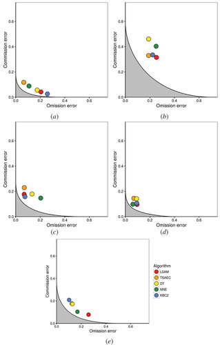
In the omission–commission space, methods are generally located close to the boundary and perform similarly. The Brazilian site, already difficult to map (see Tables 3 and 5), is the one with both the largest distances from classifications to the boundary and the highest method variability in accuracy. This is probably due to (i) double cropping systems, e.g. sugarcane, and (ii) the presence of vegetation with similar spectral-temporal signature as cropland such as grasslands, orchards, and other plantations. Forest plantations, mainly eucalyptus and pines, also share a large part of the area, and are harvested by clear cuts, and could therefore lead to confusions with other land cover during the first months of the growth.

If no one method consistently Pareto-dominates the others, it is worth noting that methods differ by their respective omission and commission error pairs as clearly illustrated for the Ukrainian and Argentinian sites (Figure 4(a, and e)). However, omission and commission error patterns remain hardly identifiable. According to the Pareto boundaries, commission error of DT method in Brazil JECAM site exceeds to 45% which are much larger than that of other four sites. The main reason is the low discrepancy of NDVI development profile between cropland and other vegetation including trees. The TSAEC method is consistently less affected by omission errors.

To evaluate the performance of a method regardless of the low-resolution bias, the minimum distance from its OE/CE pair to the boundary was evaluated. The minimum distance was chosen because an objective criterion must not penalize one specific type of error more than the other. Sites with the largest area under the curve show the largest distances to the boundary (Figure 5). More importantly, discarding the errors due the spatial resolution confirms the site-dependent character of the accuracies. Besides, it provides solid grounds to say that characteristics of the agrosystems such as the crop diversity and proportions explains another part of the accuracy rather than only the cropland fragmentation.

Figure 5. Minimum distance to the Pareto boundary for each site and method. These distances highlight the sole performance of the algorithm, regardless of the spatial resolution bias. The site effect was found statistically different whereas the method effect was not.

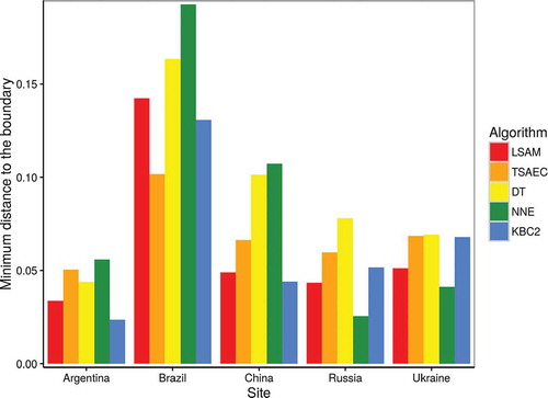
The statistical significance of the site effect on the minimum distance to the Pareto boundary was assessed using the Kruskal–Wallis test. The associated -value for the site effect reached 0.0068: at the 0.05 significance level, one may conclude for a statistically significant effect of the site. In contrast, no significant effect for the methods was found (-value = 0.5984).

4.4. Spatial agreement

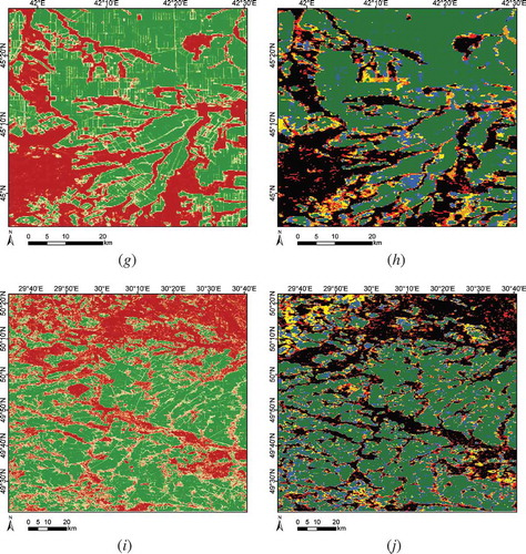
Spatial method agreement between methods was assessed by combining the different cropland masks (Figure 6(b,d,f),h),j)). The agreement was measured as the number of methods mapping a pixel as being cropland. Discrepancies ought to be related to pixel-level cropland proportions as estimated from the high-resolution reference maps (Figure 6(a,c,e,g,e)).

Figure 6. Cropland proportions derived from the high-resolution reference maps for (a) Argentina, (c) Brazil, (e) China, (g) Russia, and (i) Ukraine, and agreement maps among classification methods for (b) Argentina, (d) Brazil, (f) China, (h) Russia, and (j) Ukraine. Grey areas correspond to no data.

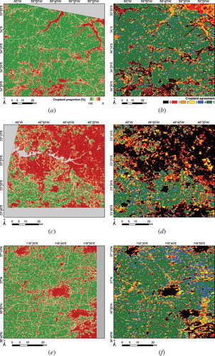
Figure 6. (Continued).

Most disagreements occur at the fringes of cropland patches. In Ukraine, the consistency patterns between methods might be divided into two parts. On the one hand, the northern quarter of the area is dominated by low cropland agreement (reddish shades). On the other hand, high agreement is observed in the remaining parts; disagreements mostly occur at class boundaries. Most disagreement occurred in areas close to water objects, e.g. rivers, lakes, and wetlands, where grassland is usually located. Due to proximity to water, grassland appears to be a very healthy vegetation and similar to summer crops, and therefore a major cause for disagreement.

In Argentina, methods display large agreement for most landscapes and each algorithm is associated with a specific commission/omission rate. Disagreement mostly occurs over non-cropland areas, particularly on the northeast side where cropland is highly overestimated (not covered with the Pareto boundary). In this area there exist lowlands mostly covered by natural vegetation that could be flooded during part of the year generating anomalies over NDVI time series and confusion in the classification methods. When compared to the high-resolution imagery and classification, it clearly becomes visible that some methods mix up grassland with cropland.

In Brazil, all methods tend to agree when the cropland dominates the landscape. But in more fragmented areas such as in the northern area of the site, most methods underestimate the cropland.

Method agreement in China is high: the landscape is well captured in every case. Most of the omission and commission errors are located at the edge of cropland patches. An identical accuracy is achieved using Neural Network Ensemble (NNE), DT, and LSAM method. Producers’ accuracy for non-cropland using KBC method ranks as lowest, but still exceeds 80%. Producers’ for cropland using NNE method ranks as highest (97%). As shown in the cropland agreement map, the discrepancy of cropland identified by four different methods is mainly located at the border of cropland and non-cropland as well as regions in the northeast. The mixture of cropland and non-cropland results in the disagreement of the cropland.

Given the large field size and the relatively simple landscape of the Russian site, a broad agreement between methods can be observed. Commission errors might be observed (red-orange shades) in the south part of the area where grassland is mistaken for cropland.

4.5. Sensitivity to the quantity of training data

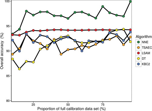
Information on the sensitivity of the classification accuracy to the amount of training data used to calibrate the classifier is useful to assess the feasibility of applying the method at a larger scale. This is demonstrated here through a systematic reduction of the calibration data set and the assessment of the resulting overall accuracy. It can be seen that with only 20% of calibration set (830 calibration pixels), four methods (NNE, LSAM, KBC, and TSAEC) reach their overall accuracy saturation plateau (98%, 95%, 92%, and 92%, respectively) (Figure 7). Therefore, estimates show that having samples that cover about 2% of the study area would be enough to achieve reasonable accuracy. The DT method requires 30% of the training data set to reach its plateau (1250 calibration pixels). Judging by the smoothness of the curves, the LSAM and DT methods display a more stable behaviour with very limited variations for the LSAM method. LSAM uses simple temporal features tailored to force close-to-normal classes local distributions, which in turn, encourage almost any kind of classifier to be used. This explains the narrow variability of the bootstrap curve: once the parameters of the distribution are calculated: they expect to change slightly with the sample size. Future work would examine the effect of different specific land cover/crop type proportion to the accuracy.

Figure 7. Dependency of average OA for testing set on training size (expressed as percentage of full training size) for JECAM site in Ukraine. The full training data set is made of 4180 pixels. Methods reach their accuracy plateau with only 20–30% of the full calibration data set (830–1250 calibration pixels).

5. Discussion

High accuracies were attained across sites for all methods (90% on average) and the classified patterns were consistent with high-resolution cropland maps. All methods show potential for larger application with different potential evolutions. The KBC², TSAEC, DT, and LSAM approaches all rely on time-series for temporal feature extraction. Temporal feature extraction requires dense and consistent time-series with good atmospheric correction and efficient cloud/shadow and snow masking. Otherwise, the resulting features would be affected by residual noise, thus degrading the quality of the classification. Data availability in areas with persistent cloud cover might be too scarce to ensure a proper temporal feature extraction, which would in turn bring down the classification accuracy. Data fusion or multi-sensor time-series is a sound way forward to increase the temporal frequency of data.

LSAM is being successfully used to map arable lands of Russia, which covers large variety of soils, agro-climatic conditions, and farming techniques both in Europe and in Asia. LSAM utilizes LAGMA, which automatically slices territory into cells of regular grid and aggregates training data of the cells’ surroundings, following cell classification. Though Russia-level overall accuracy is 92% and LSAM works well at all local test sites, it surely would encounter new challenges at global scale, like unexpected farming techniques and shifted seasonality, which probably provoke the demand on new metrics, more versatile than the ones being used.

The density of training data might introduce some overfitting effects. Specific measures were also taken in the algorithm design itself to limit the overfitting. In the NNE case for instance, the number of neurons in the neural networks was kept relatively small (10, 20, 30, and 40) and a procedure of early stopping was applied. The high levels of accuracy achieved might be downgraded when applied to larger areas. Methods showed a high stability in the level of accuracy obtained while reducing systematically the amount of calibration data. Twenty percent of the calibration set – 2% of the site’s surface – were necessary to reach the accuracy saturation plateau. In addition, DT and LSAM displayed a narrow variability of the overall accuracy.

When dealing with large volumes of satellite data, the processing time might become a critical parameter guiding method selection. Neural networks are fast to process new data but the training phase is resource- and time-consuming. Similarly, bootstrapping approaches such as TSAEC avoid random sampling anomalies and provides a proxy for the spatial variability of the classification accuracy. Yet, this comes at a higher cost in terms of processing time.

A higher spatial resolution time-series would be required for application in a more fragmented landscape. Landsat-8, Satellite HJ-1 CCD, and Sentinel-2 data have a good potential, especially if combined. As those satellites acquire data in a larger number of spectral bands than the 250 m MODIS, algorithms relying on reflectance data (NNE, KBC²) might see their accuracy increase consequently. Other methods relying on vegetation index solely would not benefit from wider spectral information.

The differences observed for the five methods in terms of spatial discrepancies and accuracy figures are good grounds for considering that two determinant factors for cropland identification are (1) the landscape fragmentation and (2) the specificity of the agrosystems in terms of land cover/crop type diversity and proportions rather than the algorithm itself. It should be noted that the impact of satellite data quality (number of available composites, number of images per composites, residual aerosol effect, omitted cloud, shadow, or snow pixels) could also partly explain the differential performance across sites. In addition, due to its whiskbroom design, the observation geometry of the MODIS instrument can result in different physical areas being mapped onto the same pixel depending on the view zenith angle (Tan et al. 2006; Campagnolo and Montano 2014). As a result, a noisy time series indicates instead a transition zone between different land uses or between fields with different management practices (Duveiller, Lopez-Lozano, and Cescatti 2015). The proportion of pure pixels might differ from site to site, which could in turn affect the accuracy of the maps. Future work could focus on integrating sub-pixel homogeneity information as proxy of pixel purity to enhance the classification accuracy.

A key finding is that the site effect dominates the method effect. On the one hand, pairwise error rates were generally found to be statistically significant but they erratically vary from one site to another. On the other hand, the site effect on the overall accuracy and the -score was statistically significant whereas the method effect was not. This effect was further confirmed when considering distances to the Pareto boundary. For regional to continental and global ambitions, this finding highlights the importance of testing a classifier over different cropping systems. This result also points out that a sensible way to derive a reliable global cropland map is to combine multiple classification approaches according to their ability to derive accurate maps in specific regions. One could thus imagine a framework in which cropland classification methods would be activated regionally according to the cloudiness, field size, landscape fragmentation, crop diversity etc. to better handle the large diversity of agrosystems. For example, NNE could be activated in cloudy areas as it would exploit and restore spectral information; TSAEC could be implemented in areas with dense time-series and where omission errors have to be minimized; LSAM could be implemented over large areas where the cropland extent is stable and where training data is scarce, etc. Manual stratification, splitting into homogeneous segments or automated spatially regular zonation could be the ways forward to identifying classifier location.

Most landscapes were dominated by cropland (Brazil being an exception) and significant discrepancies were found in fragmented areas, e.g. the northern part of the Ukrainian site and the Brazilian site. Mixed edge pixels lead to either contraction or overestimation of the cropland areas and are responsible for a large part of the classification errors. Similarly, this study highlighted that accurate cropland mapping is achievable with MODIS over fields of 20 ha or larger. In case of large homogeneous landscapes such as the North China plains where very small but adjacent fields planted with the same crop and similar management practices tend to behave like large fields (and hence have homogeneous spectral responses), the field size can go down to less than one hectare. The resolution bias accounts for 10–30% of the errors according to the cropland fragmentation. In the same vein, Wardlow and Egbert (2008) showed that MODIS time-series could provide accurate (94%) cropland maps in areas with an average field size of 32 ha or larger. It is interesting that Doraiswamy et al. (2004) reported that MODIS 250 m resolution images are adequate to monitor field sizes larger than 25 ha. In the fragmented landscapes of West Africa, Vintrou et al. (2012a) reported that a crop patch needs to be eight times larger than 25 ha in order to be detected by MODIS NDVI time series. Information on global field size, e.g. Fritz et al. (2015), is a valuable source of information to infer the areas where such accuracy could be achieved with the methods and data considered. Besides extension to larger areas around the study sites, agrosystems in Eurasia, Australia, North America (USA and Canada) as well as intensive production areas in southern Africa meet the field size requirements. Interestingly, some land covers were consistently prone to classification errors across sites. Grassland was confused with cropland is Argentina, Ukraine, and Russia, which led to an overestimation of the cropland extent. Similarly, areas close to water objects such as wetland were mapped as cropland by several methods.

Complementary to a classifier calibrated with in situ observations, classifiers could also be trained with existing land-cover maps as a default source of training data when field data are not available (see, for instance, Waldner, Canto, and Defourny 2015). There are numerous candidate land-cover maps to be considered as source (Waldner et al. 2015b); they cover the entire globe, which makes this approach suitable for large-scale and annual cropland mapping, e.g. in the Sahel region (Lambert, Waldner, and Defourny 2016).

Finally, it is recommended that future comparison studies constrain part of the sampling of validation data to error-prone areas such as class boundaries and account for class proportions. This recommendation concurs with the findings of Sweeney and Evans (2012) who highlighted substantial differences between edge and interior pixels. This approach requires that the validation data is collected after the production of the map or implies the use of existing ancillary data. Amongst the accuracy measures used, the overall accuracy and the -scores were found to be the most interesting and useful for method assessment and comparison. Studies using medium-resolution times-series are encouraged to work with the Pareto boundary as it decouples the error due to the algorithm itself and those due to the resolution. Finally, a way forward towards method comparison is certainly to compare the maps based on pixel-level uncertainty in the class attribution and to relate the spatial measure of uncertainty/accuracy to spatial characteristics of the landscape (see Löw et al. (2013); Löw, Knöfel, and Conrad (2015); Waldner, Canto, and Defourny (2015); Lambert, Waldner, and Defourny (2016) for instance).

6. Conclusions

Given the importance of accurate cropland information for crop monitoring, this study compares five existing cropland mapping methodologies in five contrasting agrosystems. Each of these methods relies on a specific set of satellite-derived features and classifiers. They were tested using 7-day 250 m MODIS mean composites (red and near-infrared channels and derived indices). In order to isolate the effect of the methodologies, input satellite data as well as calibration and validation data were identical. Overall accuracies ranged from 85% to 95% and displayed statistically significant difference in error rates. Results confirm that, from a global mapping point of view, methods’ performances vary from one agrosystem to another as a function of (1) their cropland fragmentation and (2) other specific characteristics. The origin and influence of these peculiarities such as soil type, crop diversity, cloud frequency amongst others should be studied in future works. This study highlights the need to demonstrate the performance of a method over multiple sites as results significantly vary accordingly. All five methods have potential for mapping at larger scale as they provided accurate results with 20% of the calibration data – 2% of the study area in Ukraine. Furthermore, the 250 m spatial resolution has been found suitable to provide accurate cropland maps over fields of 20 ha or larger. In case of homogeneous landscapes the field size can go down to less than one hectare such as in the China site. To conclude, this work illustrates that the site effect clearly dominates the method effect even though (1) some method–site interaction exists and (2) the landscape of all sites was dominated by agriculture. Hence, results promotes the use of a set of cropland classification methods to better address the global cropping system diversity. Thus, a sensible strategy to improve the global cropland map would be to combine regionally selected methods according to their ability to perform accurately in specific landscapes.

Acknowledgements

The authors thank the anonymous reviewers who helped to improve the quality of the manuscript. This research was conducted in the framework of the SIGMA project funded by the European Commission in the Seventh Programme for research, technological development, and demonstration under grant agreement no. 603719. The authors also thank the JECAM network for making possible this cross-site study opportunity. The arable lands mapping over the Russian Federation was supported by the Russian Science Foundation under grant number 14-17-00389.

Disclosure statement

No potential conflict of interest was reported by the authors.

Additional information

Funding

This work was supported by the European Commission in the Seventh Programme for research, technological development, and demonstration under [grant agreement No 603719] and the Russian Science Foundation under [grant number 14-17-00389].

References

- Alcantara, C., T. Kuemmerle, A. V. Prishchepov, and V. C. Radeloff. 2012. “Mapping Abandoned Agriculture with Multi-Temporal MODIS Satellite Data.” Remote Sensing of Environment 124: 334–347. doi:10.1016/j.rse.2012.05.019.
- Allen, J. D. 1990. “A Look at the Remote Sensing Applications Program of the National Agricultural Statistics Service.” Journal of Official Statistics 6 (4): 393–409.
- Arvor, D., M. Meirelles, V. Dubreuil, A. Bégué, and Y. E. Shimabukuro. 2012. “Analyzing the Agricultural Transition in Mato Grosso, Brazil, Using Satellite-Derived Indices.” Applied Geography 32 (2): 702–713. doi:10.1016/j.apgeog.2011.08.007.
- Barrett, E. C. 2013. Introduction to Environmental Remote Sensing. New York: Routledge.
- Bartalev, S. A., V. A. Egorov, D. V. Ershov, A. S. Isaev, E. A. Loupian, D. E. Plotnikov, and I. A. Uvarov. 2011. “The Vegetation Mapping over Russia Using MODIS Spectroradiometer Satellite Data.” Contemporary Earth Remote Sensing From Space 8: 285–302.
- Bartalev, S. A., V. A. Egorov, E. A. Loupian, and S. A. Khvostikov. 2014. “A New Locally-Adaptive Classification Method LAGMA for Large-Scale Land Cover Mapping Using Remote-Sensing Data.” Remote Sensing Letters 5 (1): 55–64. doi:10.1080/2150704X.2013.870675.
- Bartalev, S. A., D. E. Plotnikov, and E. A. Loupian. 2016. “Mapping of Arable Land in Russia Using Multi-Year Time Series of MODIS Data and the LAGMA Classification Technique.” Remote Sensing Letters 7 (3): 269–278. doi:10.1080/2150704X.2015.1130874.
- Battese, G. E., R. M. Harter, and W. A. Fuller. 1988. “An Error-Components Model for Prediction of County Crop Areas Using Survey and Satellite Data.” Journal of the American Statistical Association 83 (401): 28–36. doi:10.1080/01621459.1988.10478561.
- Benz, U. C., P. Hofmann, G. Willhauck, I. Lingenfelder, and M. Heynen. 2004. “Multi-Resolution, Object-Oriented Fuzzy Analysis of Remote Sensing Data for GIS-Ready Information.” ISPRS Journal of Photogrammetry and Remote Sensing 58 (3–4): 239–258. doi:10.1016/j.isprsjprs.2003.10.002.
- Biradar, C. M., P. S. Thenkabail, P. Noojipady, Y. Li, V. Dheeravath, H. Turral, M. Velpuri, et al. 2009. “A Global Map of Rainfed Cropland Areas (GMRCA) at the End of Last Millennium Using Remote Sensing.” International Journal of Applied Earth Observation and Geoinformation 11 (2): 114–129. doi:10.1016/j.jag.2008.11.002.
- Boryan, C., Z. Yang, R. Mueller, and M. Craig. 2011. “Monitoring US Agriculture: The US Department of Agriculture, National Agricultural Statistics Service, Cropland Data Layer Program.” Geocarto International 26 (5): 341–358. doi:10.1080/10106049.2011.562309.
- Boschetti, L., S. P. Flasse, and P. A. Brivio. 2004. “Analysis of the Conflict Between Omission and Commission in Low Spatial Resolution Dichotomic Thematic Products: The Pareto Boundary.” Remote Sensing of Environment 91 (3–4): 280–292. doi:10.1016/j.rse.2004.02.015.
- Breiman, L. 2001. “Random Forests.” Machine Learning 45 (1): 5–32. doi:10.1023/A:1010933404324.
- Campagnolo, M. L., and E. L. Montano. 2014. “Estimation of Effective Resolution for Daily MODIS Gridded Surface Reflectance Products.” IEEE Transactions on Geoscience and Remote Sensing 52 (9): 5622–5632. doi:10.1109/TGRS.2013.2291496.
- Caputo, B., K. Sim, F. Furesjo, and A. Smola. 2002. “Appearance-based Object Recognition using SVMs: Which Kernel Should I Use?” Proceedings of NIPS Workshop on Statistical Methods for Computational Experiments in Visual Processing and Computer Vision, Whistler, Vol. 2002.
- Champagne, C., H. McNairn, B. Daneshfar, and J. Shang. 2014. “A Bootstrap Method for Assessing Classification Accuracy and Confidence for Agricultural Land Use Mapping in Canada.” International Journal of Applied Earth Observation and Geoinformation 29: 44–52. doi:10.1016/j.jag.2013.12.016.
- Chen, B., F. Qiu, B. Wu, and H. Du. 2015. “Image Segmentation Based on Constrained Spectral Variance Difference and Edge Penalty.” Remote Sensing 7 (5): 5980–6004. doi:10.3390/rs70505980.
- Conrad, C., R. R. Colditz, S. Dech, D. Klein, and P. L. G. Vlek. 2011. “Temporal Segmentation of MODIS Time Series for Improving Crop Classification in Central Asian Irrigation Systems.” International Journal of Remote Sensing 32 (23): 8763–8778. doi:10.1080/01431161.2010.550647.
- Conrad, C., S. Dech, O. Dubovyk, S. Fritsch, D. Klein, F. Löw, G. Schorcht, and J. Zeidler. 2014. “Derivation of Temporal Windows for Accurate Crop Discrimination in Heterogeneous Croplands of Uzbekistan Using Multitemporal Rapideye Images.” Computers and Electronics in Agriculture 103: 63–74. doi:10.1016/j.compag.2014.02.003.
- Conrad, C., S. Fritsch, J. Zeidler, G. Rücker, and S. Dech. 2010. “Per-Field Irrigated Crop Classification in Arid Central Asia Using SPOT and ASTER Data.” Remote Sensing 2 (4): 1035–1056. doi:10.3390/rs2041035.
- Cushnie, J. L. 1987. “The Interactive Effect of Spatial Resolution and Degree of Internal Variability within Land-Cover Types on Classification Accuracies.” International Journal of Remote Sensing 8 (1): 15–29. doi:10.1080/01431168708948612.
- Definiens, A. G. 2009. Definiens Ecognition Developer 8 User Guide. Munchen, Germany: Definens AG.
- Delrue, J., L. Bydekerke, H. Eerens, S. Gilliams, I. Piccard, and E. Swinnen. 2013. “Crop Mapping in Countries with Small-Scale Farming: A Case Study for West Shewa, Ethiopia.” International Journal of Remote Sensing 34 (7): 2566–2582. doi:10.1080/01431161.2012.747016.
- Dheeravath, V., P. S. Thenkabail, G. Chandrakantha, P. Noojipady, G. P. O. Reddy, C. M. Biradar, M. K. Gumma, and M. Velpuri. 2010. “Irrigated Areas of India Derived Using MODIS 500 M Time Series for the Years 2001–2003.” ISPRS Journal of Photogrammetry and Remote Sensing 65 (1): 42–59. doi:10.1016/j.isprsjprs.2009.08.004.
- Doraiswamy, P. C., J. L. Hatfield, T. J. Jackson, B. Akhmedov, J. Prueger, and A. Stern. 2004. “Crop Condition and Yield Simulations Using Landsat and MODIS.” Remote Sensing of Environment 92 (4): 548–559. doi:10.1016/j.rse.2004.05.017.
- Duveiller, G., and P. Defourny. 2010. “A Conceptual Framework to Define the Spatial Resolution Requirements for Agricultural Monitoring Using Remote Sensing.” Remote Sensing of Environment 114 (11): 2637–2650. doi:10.1016/j.rse.2010.06.001.
- Duveiller, G., R. Lopez-Lozano, and A. Cescatti. 2015. “Exploiting the Multi-Angularity of the MODIS Temporal Signal to Identify Spatially Homogeneous Vegetation Cover: A Demonstration for Agricultural Monitoring Applications.” Remote Sensing of Environment 166: 61–77. doi:10.1016/j.rse.2015.06.001.
- Estel, S., T. Kuemmerle, C. Alcántara, C. Levers, A. Prishchepov, and P. Hostert. 2015. “Mapping Farmland Abandonment and Recultivation across Europe Using MODIS NDVI Time Series.” Remote Sensing of Environment 163: 312–325. doi:10.1016/j.rse.2015.03.028.
- Foerster, S., K. Kaden, M. Foerster, and S. Itzerott. 2012. “Crop Type Mapping Using Spectral–Temporal Profiles and Phenological Information.” Computers and Electronics in Agriculture 89: 30–40. doi:10.1016/j.compag.2012.07.015.
- Foley, J. A., N. Ramankutty, K. A. Brauman, E. S. Cassidy, J. S. Gerber, M. Johnston, N. D. Mueller, et al. 2011. “Solutions for a Cultivated Planet.” Nature 478 (7369): 337–342. doi:10.1038/nature10452.
- Fritz, S., and L. See. 2008. “Identifying and Quantifying Uncertainty and Spatial Disagreement in the Comparison of Global Land Cover for Different Applications.” Global Change Biology 14 (5): 1057–1075. doi:10.1111/j.1365-2486.2007.01519.x.
- Fritz, S., L. See, I. McCallum, L. You, A. Bun, E. Moltchanova, M. Duerauer, et al. 2015. “Mapping Global Cropland and Field Size.” Global Change Biology 21 (5): 1980–1992. doi:10.1111/gcb.12838.
- Fritz, S., L. See, and F. Rembold. 2010. “Comparison of Global and Regional Land Cover Maps with Statistical Information for the Agricultural Domain in Africa.” International Journal of Remote Sensing 31 (9): 2237–2256. doi:10.1080/01431160902946598.
- Gallego, F. J., N. Kussul, S. Skakun, O. Kravchenko, A. Shelestov, and O. Kussul. 2014. “Efficiency Assessment of Using Satellite Data for Crop Area Estimation in Ukraine.” International Journal of Applied Earth Observation and Geoinformation 29: 22–30. doi:10.1016/j.jag.2013.12.013.
- Giri, C., B. Pengra, J. Long, and T. R. Loveland. 2013. “Next Generation of Global Land Cover Characterization, Mapping, and Monitoring.” International Journal of Applied Earth Observation and Geoinformation 25: 30–37. doi:10.1016/j.jag.2013.03.005.
- Hammond, T. O., and D. L. Verbyla. 1996. “Optimistic Bias in Classification Accuracy Assessment.” International Journal of Remote Sensing 17 (6): 1261–1266. doi:10.1080/01431169608949085.
- Hannerz, F., and A. Lotsch. 2006. Assessment of Land Use and Cropland Inventories for Africa. CEEPA Discussion Papers 22. Pretoria: Centre of Environmental Economics and Policy in Africa, University of Pretoria.
- Husak, G. J., M. T. Marshall, J. Michaelsen, D. Pedreros, C. Funk, and G. Galu. 2008. “Crop Area Estimation Using High and Medium Resolution Satellite Imagery in Areas with Complex Topography.” Journal of Geophysical Research: Atmospheres (1984–2012) 113 (D14). doi:10.1029/2007JD009175.
- Jönsson, P., and L. Eklundh. 2004. “TIMESAT–A Program for Analyzing Time-Series of Satellite Sensor Data.” Computers & Geosciences 30 (8): 833–845. doi:10.1016/j.cageo.2004.05.006.
- Justice, C, P. Defourny, et al. 2007. “Developing a Strategy for Global Agricultural Monitoring in the Framework of Group on Earth Observations (GEO) Workshop Report.” In GEOSS Operational Agricultural Monitoring System. Rome: Food and Agriculture Organization.
- Kruskal, W. H., and W. Allen Wallis. 1952. “Use of Ranks in One-Criterion Variance Analysis.” Journal of the American Statistical Association 47 (260): 583–621. doi:10.1080/01621459.1952.10483441.
- Kussul, N., S. Skakun, A. Shelestov, M. Lavreniuk, B. Yailymov, and O. Kussul. 2015. “Regional Scale Crop Mapping Using Multi-Temporal Satellite Imagery.” ISPRS - International Archives of the Photogrammetry, Remote Sensing and Spatial Information Sciences XL-7/W3: 45–52. doi:10.5194/isprsarchives-XL-7-W3-45-2015.
- Kussul, N., S. Skakun, A. Shelestov, and O. Kussul. 2014. “The Use of Satellite SAR Imagery to Crop Classification in Ukraine within JECAM Project.” In Geoscience and Remote Sensing Symposium (IGARSS), 2014 IEEE International, 1497–1500. IEEE.
- Lambert, M.-J., F. Waldner, and P. Defourny. 2016. “Cropland Mapping over Sahelian and Sudanian Agrosystems: A Knowledge-Based Approach Using PROBA-V Time Series at 100-m.” Remote Sensing 8 (3): 232. doi:10.3390/rs8030232.
- Latif, B. A., R. Lecerf, G. Mercier, and L. Hubert-Moy. 2008. “Preprocessing of Low-Resolution Time Series Contaminated by Clouds and Shadows.” IEEE Transactions on Geoscience and Remote Sensing 46 (7): 2083–2096. doi:10.1109/TGRS.2008.916473.
- Li, J., X. Chen, L. Tian, J. Huang, and L. Feng. 2015. “Improved Capabilities of the Chinese High-Resolution Remote Sensing Satellite GF-1 for Monitoring Suspended Particulate Matter (SPM) in Inland Waters: Radiometric and Spatial Considerations.” ISPRS Journal of Photogrammetry and Remote Sensing 106: 145–156. doi:10.1016/j.isprsjprs.2015.05.009.
- Löw, F., U. Michel, S. Dech, and C. Conrad. 2013. “Impact of Feature Selection on the Accuracy and Spatial Uncertainty of Per-Field Crop Classification Using Support Vector Machines.” ISPRS Journal of Photogrammetry and Remote Sensing 85: 102–119. doi:10.1016/j.isprsjprs.2013.08.007.
- Löw, F., and G. Duveiller. 2014. “Defining the Spatial Resolution Requirements for Crop Identification Using Optical Remote Sensing.” Remote Sensing 6 (9): 9034–9063. doi:10.3390/rs6099034.
- Löw, F., P. Knöfel, and C. Conrad. 2015. “Analysis of Uncertainty in Multi-Temporal Object-Based Classification.” ISPRS Journal of Photogrammetry and Remote Sensing 105: 91–106. doi:10.1016/j.isprsjprs.2015.03.004.
- Mallinis, G., and N. Koutsias. 2012. “Comparing Ten Classification Methods for Burned Area Mapping in a Mediterranean Environment Using Landsat TM Satellite Data.” International Journal of Remote Sensing 33 (14): 4408–4433. doi:10.1080/01431161.2011.648284.
- Matton, N., G. S. Canto, F. Waldner, S. Valero, D. Morin, J. Inglada, M. Arias, S. Bontemps, B. Koetz, and P. Defourny. 2015. “An Automated Method for Annual Cropland Mapping along the Season for Various Globally-Distributed Agrosystems Using High Spatial and Temporal Resolution Time Series.” Remote Sensing 7 (10): 13208–13232. doi:10.3390/rs71013208.
- McNemar, Q. 1947. “Note on the Sampling Error of the Difference between Correlated Proportions or Percentages.” Psychometrika 12 (2): 153–157. doi:10.1007/BF02295996.
- Meier, U., D. C. Ciresan, L. M. Gambardella, and J. Schmidhuber. 2011. “Better Digit Recognition with a Committee of Simple Neural Nets.” In 2011 International Conference on Document Analysis and Recognition (ICDAR), 1250–1254. IEEE.
- Meng, J., X. Du, and B. Wu. 2013. “Generation of High Spatial and Temporal Resolution NDVI and Its Application in Crop Biomass Estimation.” International Journal of Digital Earth 6 (3): 203–218. doi:10.1080/17538947.2011.623189.
- Miao, Z., L. Qiangzi, and W. Bingfang. 2012. “Investigating the Capability of Multi-Temporal Landsat Images for Crop Identification in High Farmland Fragmentation Regions.” In 2012 First International Conference on Agro-Geoinformatics (Agro-Geoinformatics), 1–4. IEEE.
- Millard, K., and M. Richardson. 2015. “On the Importance of Training Data Sample Selection in Random Forest Image Classification: A Case Study in Peatland Ecosystem Mapping.” Remote Sensing 7 (7): 8489–8515. doi:10.3390/rs70708489.
- Müller, H., P. Rufin, P. Griffiths, A. J. Siqueira, and P. Hostert. 2015. “Mining Dense Landsat Time Series for Separating Cropland and Pasture in a Heterogeneous Brazilian Savanna Landscape.” Remote Sensing of Environment 156: 490–499. doi:10.1016/j.rse.2014.10.014.
- Murakami, T., S. Ogawa, N. Ishitsuka, K. Kumagai, and G. Saito. 2001. “Crop Discrimination with Multitemporal SPOT/HRV Data in the Saga Plains, Japan.” International Journal of Remote Sensing 22 (7): 1335–1348. doi:10.1080/01431160151144378.
- Olofsson, P., S. V. Stehman, C. E. Woodcock, D. Sulla-Menashe, A. M. Sibley, J. D. Newell, M. A. Friedl, and M. Herold. 2012. “A Global Land-Cover Validation Data Set, Part I: Fundamental Design Principles.” International Journal of Remote Sensing 33 (18): 5768–5788. doi:10.1080/01431161.2012.674230.
- Ozdogan, M., and C. E. Woodcock. 2006. “Resolution Dependent Errors in Remote Sensing of Cultivated Areas.” Remote Sensing of Environment 103 (2): 203–217. doi:10.1016/j.rse.2006.04.004.
- Pan, Y., T. Hu, X. Zhu, J. Zhang, and X. Wang. 2012. “Mapping Cropland Distributions Using a Hard and Soft Classification Model.” IEEE Transactions on Geoscience and Remote Sensing 50 (11): 4301–4312. doi:10.1109/TGRS.2012.2193403.
- Peña-Barragán, J. M., M. K. Ngugi, R. E. Plant, and J. Six. 2011. “Object-Based Crop Identification Using Multiple Vegetation Indices, Textural Features and Crop Phenology.” Remote Sensing of Environment 115 (6): 1301–1316. doi:10.1016/j.rse.2011.01.009.
- Pflugmacher, D., O. N. Krankina, W. B. Cohen, M. A. Friedl, D. Sulla-Menashe, R. E. Kennedy, P. Nelson, et al. 2011. “Comparison and Assessment of Coarse Resolution Land Cover Maps for Northern Eurasia.” Remote Sensing of Environment 115 (12): 3539–3553. doi:10.1016/j.rse.2011.08.016.
- Pittman, K., M. C. Hansen, I. Becker-Reshef, P. V. Potapov, and C. O. Justice. 2010. “Estimating Global Cropland Extent with Multi-Year MODIS Data.” Remote Sensing 2 (7): 1844–1863. doi:10.3390/rs2071844.
- Plotnikov, D., S. A. Bartalev, and V. A. Egorov. 2010. “The Recognition Features to Map Arable Lands Based on Multi-Annual MODIS Earth Observation Data [In Russian].” Contemporary Remote Sensing from Space 7: 330–341.
- Pontius, R. G., and M. Millones. 2011. “Death to Kappa: Birth of Quantity Disagreement and Allocation Disagreement for Accuracy Assessment.” International Journal of Remote Sensing 32 (15): 4407–4429. doi:10.1080/01431161.2011.552923.
- Savitzky, A., and M. J. E. Golay. 1964. “Smoothing and Differentiation of Data by Simplified Least Squares Procedures.” Analytical Chemistry 36 (8): 1627–1639. doi:10.1021/ac60214a047.
- Shao, Y., and R. S. Lunetta. 2012. “Comparison of Support Vector Machine, Neural Network, and CART Algorithms for the Land-Cover Classification Using Limited Training Data Points.” ISPRS Journal of Photogrammetry and Remote Sensing 70: 78–87. doi:10.1016/j.isprsjprs.2012.04.001.
- Shelestov, A. Y., A. N. Kravchenko, S. V. Skakun, S. V. Voloshin, and N. N. Kussul. 2013. “Geospatial Information System for Agricultural Monitoring.” Cybernetics and Systems Analysis 49 (1): 124–132. doi:10.1007/s10559-013-9492-5.
- Shen, J., J. Liu, X. Lin, R. Zhao, and S. Xu. 2011. “Cropland Extraction from Very High Spatial Resolution Satellite Imagery by Object-Based Classification Using Improved Mean Shift and One-Class Support Vector Machines.” Sensor Letters 9 (3): 997–1005. doi:10.1166/sl.2011.1361.
- Skakun, S., N. Kussul, A. Y. Shelestov, M. Lavreniuk, and O. Kussul. 2015. “Efficiency Assessment of Multitemporal C-Band Radarsat-2 Intensity and Landsat-8 Surface Reflectance Satellite Imagery for Crop Classification in Ukraine.” IEEE Journal of Selected Topics in Applied Earth Observations and Remote Sensing PP 99: 1–8.
- Skakun, S. V., and R. M. Basarab. 2014. “Reconstruction of Missing Data in Time-Series of Optical Satellite Images Using Self-Organizing Kohonen Maps.” Journal of Automation and Information Sciences 46: 19–26. doi:10.1615/JAutomatInfScien.v46.i12.
- Soares, D. de M., L. S. Galvão, and A. R. Formaggio. 2008. “Crop Area Estimate from Original and Simulated Spatial Resolution Data and Landscape Metrics.” Scientia Agricola 65 (5): 459–467. doi:10.1590/S0103-90162008000500003.
- Sweeney, S. P., and T. P. Evans. 2012. “An Edge-Oriented Approach to Thematic Map Error Assessment.” Geocarto International 27 (1): 31–56. doi:10.1080/10106049.2011.622052.
- Tan, B., C. E. Woodcock, J. Hu, P. Zhang, M. Ozdogan, D. Huang, W. Yang, Y. Knyazikhin, and R. B. Myneni. 2006. “The Impact of Gridding Artifacts on the Local Spatial Properties of MODIS Data: Implications for Validation, Compositing, and Band-To-Band Registration across Resolutions.” Remote Sensing of Environment 105 (2): 98–114. doi:10.1016/j.rse.2006.06.008.
- Thenkabail, P. S., and Z. Wu. 2012. “An Automated Cropland Classification Algorithm (ACCA) for Tajikistan by Combining Landsat, MODIS, and Secondary Data.” Remote Sensing 4 (12): 2890–2918. doi:10.3390/rs4102890.
- Tsai, F., and W. Philpot. 1998. “Derivative Analysis of Hyperspectral Data.” Remote Sensing of Environment 66 (1): 41–51. doi:10.1016/S0034-4257(98)00032-7.
- Van Niel, T. G., and T. R. McVicar. 2004. “Determining Temporal Windows for Crop Discrimination with Remote Sensing: A Case Study in South-Eastern Australia.” Computers and Electronics in Agriculture 45 (1–3): 91–108. doi:10.1016/j.compag.2004.06.003.
- Vancutsem, C., J.-F. Pekel, P. Bogaert, and P. Defourny. 2007. “Mean Compositing, an Alternative Strategy for Producing Temporal Syntheses. Concepts and Performance Assessment for SPOT VEGETATION Time Series.” International Journal of Remote Sensing 28 (22): 5123–5141. doi:10.1080/01431160701253212.
- Vancutsem, C., E. Marinho, F. Kayitakire, L. See, and S. Fritz. 2012. “Harmonizing and Combining Existing Land Cover/Land Use Datasets for Cropland Area Monitoring at the African Continental Scale.” Remote Sensing 5 (1): 19–41. doi:10.3390/rs5010019.
- Vapnik, V. 2000. The Nature of Statistical Learning Theory. New York: Springer Science & Business Media.
- Vintrou, E., A. Desbrosse, A. Bégué, S. Traoré, C. Baron, and D. L. Seen. 2012a. “Crop Area Mapping in West Africa Using Landscape Stratification of MODIS Time Series and Comparison with Existing Global Land Products.” International Journal of Applied Earth Observation and Geoinformation 14 (1): 83–93. doi:10.1016/j.jag.2011.06.010.
- Vintrou, E., D. Ienco, A. Begue, and M. Teisseire. 2013. “Data Mining, a Promising Tool for Large-Area Cropland Mapping.” IEEE Journal of Selected Topics in Applied Earth Observations and Remote Sensing 6 (5): 2132–2138. doi:10.1109/JSTARS.2013.2238507.
- Waldner, F., G. S. Canto, and P. Defourny. 2015. “Automated Annual Cropland Mapping Using Knowledge-Based Temporal Features.” ISPRS Journal of Photogrammetry and Remote Sensing 110: 1–13. doi:10.1016/j.isprsjprs.2015.09.013.
- Waldner, F., M. A. B. Ebbe, K. Cressman, and P. Defourny. 2015a. “Operational Monitoring of the Desert Locust Habitat with Earth Observation: An Assessment.” ISPRS International Journal of Geo-Information 4 (4): 2379–2400. doi:10.3390/ijgi4042379.
- Waldner, F., S. Fritz, A. D. Gregorio, and P. Defourny. 2015b. “Mapping Priorities to Focus Cropland Mapping Activities: Fitness Assessment of Existing Global, Regional and National Cropland Maps.” Remote Sensing 7 (6): 7959–7986. doi:10.3390/rs70607959.
- Waldner, F., S. Fritz, A. D. Gregorio, D. Plotnikov, S. Bartalev, N. Kussul, P. Gong, et al. 2016. “A Unified Cropland Layer at 250 m for Global Agriculture Monitoring.” Data 1 (1): 3. doi:10.3390/data1010003.
- Wardlow, B. D., and S. L. Egbert. 2008. “Large-Area Crop Mapping Using Time-Series MODIS 250 M NDVI Data: An Assessment for the US Central Great Plains.” Remote Sensing of Environment 112 (3): 1096–1116. doi:10.1016/j.rse.2007.07.019.
- Watts, J. D., R. L. Lawrence, P. R. Miller, and C. Montagne. 2009. “Monitoring of Cropland Practices for Carbon Sequestration Purposes in North Central Montana by Landsat Remote Sensing.” Remote Sensing of Environment 113 (9): 1843–1852. doi:10.1016/j.rse.2009.04.015.
- Wu, W., R. Shibasaki, P. Yang, Q. Zhou, and H. Tang. 2008. “Remotely Sensed Estimation of Cropland in China: A Comparison of the Maps Derived from Four Global Land Cover Datasets.” Canadian Journal of Remote Sensing 34 (5): 467–479. doi:10.5589/m08-059.
- Wu, Z., P. S. Thenkabail, R. Mueller, A. Zakzeski, F. Melton, L. Johnson, C. Rosevelt, J. Dwyer, J. Jones, and J. P. Verdin. 2014. “Seasonal Cultivated and Fallow Cropland Mapping Using MODIS-Based Automated Cropland Classification Algorithm.” Journal of Applied Remote Sensing 8 (1): 083685–083685. doi:10.1117/1.JRS.8.083685.
- Xiao, X., S. Boles, J. Liu, D. Zhuang, S. Frolking, C. Li, W. Salas, and B. Moore. 2005. “Mapping Paddy Rice Agriculture in Southern China Using Multi-Temporal MODIS Images.” Remote Sensing of Environment 95 (4): 480–492. doi:10.1016/j.rse.2004.12.009.
- Zhong, L., P. Gong, and G. S. Biging. 2014. “Efficient Corn and Soybean Mapping with Temporal Extendability: A Multi-Year Experiment Using Landsat Imagery.” Remote Sensing of Environment 140: 1–13. doi:10.1016/j.rse.2013.08.023.