Retrieval of suspended particulate matter from turbidity – model development, validation, and application to MERIS data over the Baltic Sea

ABSTRACT

Suspended particulate matter (SPM) causes most of the scattering in natural waters and thus has a strong influence on the underwater light field, and consequently on the whole ecosystem. Turbidity is related to the concentration of SPM which usually is measured gravimetrically, a rather time-consuming method. Measuring turbidity is quick and easy, and therefore also more cost-effective. When derived from remote sensing data the method becomes even more cost-effective because of the good spatial resolution of satellite data and the synoptic capability of the method. Turbidity is also listed in the European Union’s Marine Strategy Framework Directive as a supporting monitoring parameter, especially in the coastal zone. In this study, we aim to provide a new Baltic Sea algorithm to retrieve SPM concentration from in situ turbidity and investigate how this can be applied to satellite data. An in situ dataset was collected in Swedish coastal waters to develop a new SPM model. The model was then tested against independent datasets from both Swedish and Lithuanian coastal waters. Despite the optical variability in the datasets, SPM and turbidity were strongly correlated (r = 0.97). The developed model predicts SPM reliably from in situ turbidity (R² = 0.93) with a mean normalized bias (MNB) of 2.4% for the Swedish and 14.0% for the Lithuanian datasets, and a relative error (RMS) of 25.3% and 37.3%, respectively. In the validation dataset, turbidity ranged from 0.3 to 49.8 FNU (Formazin Nephelometric Unit) and correspondingly, SPM concentration ranged from 0.3 to 34.0 g m^–3 which covers the ranges typical for Baltic Sea waters. Next, the medium-resolution imaging spectrometer (MERIS) standard SPM product MERIS Ground Segment (MEGS) was tested on all available match-up data (n = 67). The correlation between SPM retrieved from MERIS and in situ SPM was strong for the Swedish dataset with r = 0.74 (RMS = 47.4 and MNB = 11.3%; n = 32) and very strong for the Lithuanian dataset with r = 0.94 (RMS = 29.5% and MNB = −1.5%; n = 35). Then, the turbidity was derived from the MERIS standard SPM product using the new in situ SPM model, but retrieving turbidity from SPM instead. The derived image was then compared to existing in situ data and showed to be in the right range of values for each sub-area. The new SPM model provides a robust and cost-efficient method to determine SPM from in situ turbidity measurements (or vice versa). The developed SPM model predicts SPM concentration with high quality despite the high coloured dissolved organic matter (CDOM) range in the Baltic Sea. By applying the developed SPM model to already existing remote sensing data (MERIS/Envisat) and most importantly to a new generation of satellite sensors (in particular OLCI on board the Sentinel-3), it is possible to derive turbidity for the Baltic Sea.

1. Introduction

Natural waters contain suspended particulate matter (SPM), which affects the water quality by modifying the light field, as SPM is responsible for most of the scattering (J. T. O. Kirk 2010). The SPM concentration is a parameter of main interest for sediment transport and can also indicate transport of organic toxins (e.g. Malmaeus and Håkanson 2003; Ruddick et al. 2008). Reliable estimates of SPM concentrations are also needed as input to hydro-chemical and ecological models, for example, as a proxy for terrestrial input, re-suspension, or the sedimentation of particles (Fettweis and Van den Eynde 2003; Lindström et al. 1999; Blaas et al. 2007). SPM consists of matter kept in suspension in the surface mixed layer by physical forcing, such as currents or wind-wave stirring, and it contains both inorganic and organic material. The inorganic fraction consists mostly of mineral particles originating from river discharge and erosion (Bukata et al. 1995; Bowers and Binding 2006; J. T. O. Kirk 2010; Jerlov 1976). The organic part of SPM consists of organic detritus, plankton, and bacteria (Bukata et al. 1995; Bowers and Binding 2006; J. T. O. Kirk 2010; Jerlov 1976).

Turbidity is defined as the reduction of transparency of liquids caused by the presence of SPM (ISO 7027). Turbidity is a measure of scattering, which is directly related to the concentration of SPM (Bukata et al. 1995; Kallio 2012). Thus, turbidity can be used as an estimate of SPM concentration (Dogliotti et al. 2015; Davies-Colley and Smith 2001; Bukata et al. 1995; J. T. O. Kirk 2010). An increase in turbidity affects both the top-down and the bottom-up processes in ecosystems. Increased turbidity reduces light availability, which may limit primary production (J. T. O. Kirk 2010; Lucas et al. 1999; Davies-Colley and Smith 2001; Jassby, Cloern, and Cole 2002; Fleming and Kaitala 2006). Furthermore, increased turbidity may reduce the nutritional quality for zooplankton, for example, by increasing the amount of inorganic suspended particulate matter in comparison to phytoplankton (Arruda, Richard Marzolf, and Faulk 1983; K. L. Kirk and Gilbert 1990). On the other hand, zooplankton biomass can be positively affected, as increased turbidity reduces the predation success of visual predators (MacKenzie and KiØrboe 2000; Salonen and Engström-Öst 2013; Lunt and Smee 2014). Seasonal changes in precipitation and river discharge alter the SPM concentrations, as increased precipitation leads to increased transport of SPM loads from land to the sea (Miller and McKee 2004). Increased SPM load can also be caused by hydrodynamic activities, such as upwelling events (Suursaar et al. 2009), by erosion, and by anthropogenic causes, such as dredging. Hence, SPM concentration and turbidity are important factors for understanding these processes within the coastal zone. Furthermore, SPM can be used as an indicator of coastal dynamics and to assess the extent of the coastal zone (Kratzer and Tett 2009; Kyryliuk and Kratzer 2016).

Both SPM concentration and turbidity are important parameters describing the water quality of natural waters, and remote sensing retrieved data can provide an efficient method to monitor both (Nechad, Ruddick, and Park 2010). Turbidity is listed as one of the mandatory physical and chemical parameters to be measured within Annex III of the European Union’s Marine Strategy Framework Directive (European Commission 2008, Annex III) for the initial assessment and determination of good environmental status of every marine region or sub-region, especially in coastal waters. Moreover, the Baltic Sea is optically dominated by absorption of coloured dissolved organic matter (CDOM) (Kowalczuk, Stedmon, and Markager 2006; Kratzer and Tett 2009; Form et al. 2004). In order to avoid the effect of CDOM absorption on turbidity measurements, in this study turbidity was measured in situ according to the ISO 7027 method with portable turbidity meters. This method offers a quick and cost-effective measurement of turbidity. The in situ SPM concentration was determined gravimetrically according to Strickland and Parsons (1972). The gravimetrical method is reliable with standard errors around 10% (Kratzer 2000), but the method is rather time-consuming and hence costly. In addition to the gravimetrical method, SPM can be derived from ocean colour remote sensing data. Conventional remote sensing algorithms determine the SPM concentration based on changes either in reflectance ratios of two or more bands or in brightness through single band reflectance (Binding, Bowers, and Mitchelson-Jacob 2005). Currently, however, the methods for coastal remote sensing usually rely on more complex novel inversion techniques and/or neural network approaches (Doerffer and Schiller 2007). These methods are used to retrieve SPM concentration in optically complex waters, such as the Baltic Sea, where the optical signal of SPM does not necessarily co-vary with chlorophyll concentration. Previous studies in the NW and SE Baltic Sea (Kratzer and Vinterhav 2010; Beltrán-Abaunza, Kratzer, and Brockmann 2014; Vaičiūtė, Bresciani, and Bučas. 2012) have shown that the SPM products from the ocean colour multi-spectral spectrometer ‘medium-resolution imaging spectrometer’ (MERIS) over- or underestimate SPM concentration by about 8–16%, depending on the processor used.

The aim of this study is to provide a regional SPM model to estimate SPM concentrations from turbidity data in strongly absorbing Baltic Sea waters. We hypothesize that the regional in situ SPM model will allow us to retrieve SPM concentration reliably from in situ turbidity. In addition, we aim to retrieve turbidity from the MERIS standard SPM product using the new SPM model to illustrate the spatial changes of turbidity over the Baltic Sea.

2. Methods

2.1. In situ sampling and measurement areas

The in situ dataset was collected from several cruises in the NW Baltic Sea in Swedish coastal waters during 2008–2014 and in the Lithuanian coastal waters of the SE Baltic Sea, covering the Curonian Lagoon, during 2009–2014 (Figure 1). In Sweden, the stations were sampled along transects following a nearshore to offshore gradient. These sampling stations are part of the Swedish coastal monitoring programme. In Lithuania, the sampling stations were distributed along a salinity gradient covering fresh waters in the lagoon, a plume region with reduced salinity (4.1 ± 1.3 PSU) and brackish (6.8 ± 0.3 PSU) coastal Baltic Sea waters. Table 1 shows the measurement periods for the respective coastal areas and the number of measurements (n) per station and indicates which datasets were used for model development and validation. Water samples for SPM and turbidity analysis were sampled with a bucket just below the surface to avoid floating matter on the sea surface. The samples were analysed as soon as possible. In the Lithuanian dataset, all samples were analysed the same day, and in the Swedish dataset 76% on the same day, 22% on the next day, and 2% after 2 days. The water samples were kept cold and dark from sampling to analysis. If not analysed the same day, the samples were stored in 4°C. In the Swedish dataset, for 96% of the measurements three replicates were used for SPM and turbidity analysis, whereas 4% had only one or two replicates, due to leakage during filtration. For the measurements with one or two replicates, the values were within the range of the standard deviation of the other measurements from the same stations. Hence, the lack of replicates presumably did not affect the quality of the results. The average of the replicates represents the station value, and the method error was calculated based on the variance per station. In the Lithuanian dataset, however, only one sample was collected per station. Hence, the method error was calculated using the standard deviation of all samples.

Table 1. Measurement periods and transects from 2008 to 2014. The match-up dataset for remote sensing from 2008 to 2010 was used for comparing both the MERIS standard SPM product and the SPM retrieved with the new SPM model based on in situ data (n = 67). The dataset from 2010 to 2012 (n = 69) was used for developing a turbidity regression model, and subsequently the Swedish dataset from 2013 to 2014 (n = 45) and Lithuanian dataset from 2012 to 2014 (n = 51) were used for testing the model. Indices a–e refer to areas on Figure 1.

Year	Period	Study area	Number of measurements
2008	9–31 July	Himmerfjärden^b	21	MERIS match-up dataset
2009	14 July	Lithuanian sites	2
2010	5 June–6 September	Lithuanian sites	33
2010	5–24 May	Himmerfjärden^b	11
2010	17–20 August	Himmerfjärden^b	10	SPM model development
2011	17 July–24 August	Himmerfjärden^b/Nyköping^c/Östhammar^a	10/8/5
2012	27 April–21 May	Himmerfjärden^b	14
2012	18 June–26 July	Nyköping^c/Bråviken^d/Kaggebofjärden^e	5/12/5
2012	29–30 July	Lithuanian sites	11	SPM model validation
2013	17 June–4 September	Nyköping^c/Bråviken^d/Kaggebofjärden^e	3/15/5
2013	6 August	Lithuanian sites	11
2014	18 February–28 May	Himmerfjärden^b	22
2014	29 April–3 September	Lithuanian sites	29

Figure 1. Map of the study areas and in situ stations in the Baltic Sea. The map of the NW Baltic Sea shows the sampled Swedish area with detailed maps of the subareas denoted by the letters a–e. The map of the SE Baltic Sea shows the sampled Lithuanian area, including the Curonian Lagoon. The stations labelled CL are stations within the lagoon (marked with open circles), the stations denoted BS are brackish Baltic Sea stations (marked with filled circles) and plume stations with varying salinity (marked with plus signs). Swedish maps © Lantmäteriet, Gävle 2010; permission I2014/00691.

The northernmost area on the Swedish coast, Östhammar bay (a), is situated in the Åland Sea. All other Swedish areas are located in the north-western Baltic proper. Himmerfjärden bay (b) is located in the southern Stockholm Archipelago. The bay consists of several basins and has a relatively small water volume. In addition, there is a weak internal circulation due to low freshwater input and several sills restricting the mixing between the different basins. An urban waste water treatment plant is situated at the head of Himmerfjärden bay, and the bay serves as recipient for the effluent. Nyköping bay (c) is very shallow at the inner part, with restricted water exchange with the open sea, due to a narrow strait. This bay receives a large freshwater inflow from three rivers, causing gradients of increasing salinity and decreasing SPM concentration towards the sea. Bråviken bay (d) is a 50 km long bay, with a high freshwater inflow. Located south of the Bråviken bay, the Slätbaken bay (d) is relatively deep with sills restricting the water exchange between the bay and the open sea. Due to restricted water exchange combined with nutrient-rich freshwater inflow, Slätbaken bay is eutrophicated. Two more stations were sampled south of Slätbaken bay, Kaggebofjärden and Lindödjupet (e).

The coast of the Lithuanian Baltic Sea is often exposed to westerly winds that produce a hydrodynamically active environment with no oxygen deficiency. The Klaipeda Strait provides a narrow connection with a large, freshwater, shallow water body, the Curonian Lagoon (total area 1584 km², mean depth 3.8 m). The mixing of fresh and brackish water masses creates spatially and temporally unstable salinity gradients ranging from 0 PSU inside the lagoon to 7 PSU offshore (Dailidienė and Davulienė 2008; Vaičiūtė, Bresciani, and Bučas. 2012). The Curonian Lagoon itself has a main freshwater inlet – the Nemunas River. The river drains a large watershed, hosting wetlands and forests, and discharges annually nearly 23 km³ of CDOM-rich freshwater (Ferrarin et al. 2008). The hydrology of the lagoon varies seasonally with changes in river discharge. During elevated discharge, the northern part of the lagoon is typically defined as a transitional riverine-like system with a mixing of brackish, lagoon and riverine waters, while in the summer, there is little input from either sources.

2.2. Laboratory analysis

SPM concentrations were determined gravimetrically in the laboratory, according to Strickland and Parsons (1972). GF/F-filters (nominal pore size 0.7 μm) were pre-rinsed with 100 ml ultra-pure water, to clear off any loose filter bits and subsequently combusted at 450–480°C for 5 hours, in order to burn off any organic contamination (Doerffer 2002). The combusted filters were weighed before filtration (tare weight), after filtration and drying (dry weight) overnight and after combusting the filters again (combusted weight). The total SPM concentration is the difference between dry weight and tare weight. The inorganic SPM is the difference between combusted weight and tare weight. Thus, the organic SPM is the difference between total SPM and inorganic SPM (Strickland and Parsons 1972). The values were corrected for handling errors such as loss of filter bits or dust contamination by filtering ultra-pure water through the filter instead of a water sample, and treating the filter subsequently in the same way as all other samples. The measurements from one sampling station were excluded, as the standard deviation of the SPM concentrations was 10-fold the normal value, indicating a handling error.

Turbidity was measured with a portable turbidity meter (Hach Lange 2100Qis, Düsseldorf, Germany) in Formazin Nephelometric Unit (FNU) in Swedish coastal waters during 2010–2014 and in Lithuanian coastal waters during 2012. During 2013–2014 in Lithuania, turbidity was measured with a portable turbidity meter (Eutech Instruments TN-100, Landsmeer, The Netherlands) in Nephelometric Turbidity Unit (NTU). Both instruments have a light-emitting diode in the near-infrared range (Hach Lange at 860 nm and Eutech Instruments at 850 nm), and the detector measures the scatter at a 90° angle. This method is based on the International Standard Organisation (ISO) 7027. The light source in the near-infrared is important for waters with high CDOM absorption, since the effect of CDOM absorption is negligible in the near-infrared part of the spectrum decreasing to zero at about 750 nm. The measurement accuracy of the Hach Lange turbidity meter is ±2% and the instrument has three measuring modes. The normal mode was selected for this study, as it covered the predicted range of turbidity values (Lithner, Holm, and Ekström 2003). In this mode, the instrument takes three measurements and calculates the average value as output, with the high measurement quality up to 20 FNU. Hence, only measurements below 20 FNU were included in the SPM model development. Therefore, one measurement was excluded from the Swedish dataset: 29 July 2012 at Sö11b (21.67 FNU) in the inner Nyköping bay. Although including the station would not have affected the results as a data evaluation showed that it was in line with the rest of the data. In the SPM model validation, however all data were included. Supportive data on CDOM and chlorophyll-a (chl-a) were collected at the same time and analysed according to established methods or ISO standards (see Strickland and Parsons 1972; Jeffrey and Vesk 1997; HELCOM 2014, for chl-a analysis; J. T. O. Kirk 2010 for CDOM analysis). More detailed descriptions can be found in Kratzer and Tett (2009), Harvey, Kratzer, and Philipson (2015), and Harvey, Kratzer, and Andersson (2015).

2.3. SPM model development and validation

First, the in situ dataset from 2010 to 2012 from the NW Baltic Sea (n = 69, 28 sampling stations) was used for developing an algorithm that describes the relationship between turbidity and SPM, using a least square regression model. Then, the validity of the regression model was tested with the in situ dataset from NW Baltic Sea during 2013–2014 (n = 45) and from the SE Baltic Sea and the Curonian Lagoon collected during 2012–2014 (n = 51). The datasets were divided this way because the statistical analysis of the SPM model did not show any effects of season or organic fraction onto the SPM model. Both the model development and validation datasets covered very similar ranges of optical variables and had a large seasonal coverage. Additional variables were considered to improve the SPM model and tested statistically with ANOVA F-test or by examining the residuals.

2.4. Application to remote sensing data

In this study, MERIS full-resolution (300 m) data from the third reprocessing were used (Bourg and Members of the MERIS Quality Working Group 2011). The full-resolution scenes were processed with the Optical Data Processor of the European Space Agency (ODESA) 1.2.4/MERIS Ground Segment (MEGS) 8.1 (ACRI-ST 2012; Doerffer and Schiller 2007) to retrieve the level 2 product: the MERIS SPM standard product (total suspended matter). Next, the MERIS standard SPM product was tested against the independent match-up datasets from both geographical areas, and the RMS and MNB errors were derived. The two match-up datasets were collected during dedicated sea-truthing campaigns in the Swedish coastal waters during 2008, 2009, and 2010 (Kratzer and Vinterhav 2010; Beltrán-Abaunza, Kratzer, and Brockmann 2014) and in the Lithuanian coastal waters during 2009 and 2010 (Vaičiūtė, Bresciani, and Bučas. 2012). These match-up datasets consisted of 67 match-ups in total (Table 1), of which 32 were from the NW Baltic Sea (Beltrán-Abaunza, Kratzer, and Brockmann 2014), and 35 from the Lithuanian coast. For the validation of the algorithm, the match-up in situ data were compared with the satellite data for the corresponding pixels in a 3 × 3 matrix as simultaneously as possible. In this study, we used a time-window of ±2 hours. Surface currents can affect the validation results, but the current velocity in the Baltic Sea is rather slow compared with tidally influenced waters, and was assumed to be 5 cm s⁻¹. At this velocity, the water mass may move a maximum of 180 m in an hour, and in two hours the water mass may thus move about one MERIS pixel (Beltrán-Abaunza, Kratzer, and Brockmann 2014). Therefore, a matrix of 3 × 3 pixels centred at the field sample location should cover the natural variability of water displacement within ±2 hours. The possible boat drifting during sampling was taken into account by using the start and end locations to determine the mid-point as the sampling station. In case of multiple locations per station, the centroid of these locations was used when selecting the match-up pixel to compare with the in situ value. All geolocation calculations assume a flat surface. A quality check of the level 2 products was done according to Beltrán-Abaunza et al. (2016, this issue). Pixel values were masked out, if the value was NaN, negative or if the following level 2 flags were raised in the NetCDF file: Land, Cloud, Suspect and Ice haze. Turbidity was then retrieved from the MERIS standard SPM product using the new SPM model to illustrate the spatial variability of turbidity.

3. Results

3.1. SPM model development and validation

The SPM model was developed based on the Swedish in situ dataset from 2010 to 2012. In this dataset, the in situ turbidity ranged from 0.6 to 15.4 FNU, with a median 2.4 FNU and an average 3.6 FNU. Correspondingly, SPM concentrations varied from 0.5 to 14.9 g m⁻³ with a median value 2.0 g m⁻³ and an average 3.2 g m⁻³. The proportion of inorganic matter of the total SPM concentration ranged from 18.7% to 93.0% covering a wide range of inorganic to organic ratios. SPM concentration and turbidity were related linearly and showed a very strong correlation, with a correlation coefficient r = 0.97 (t-test; p < 0.001, n = 69) and with a coefficient of determination R² = 0.93. A linear regression model was developed with the least squares method and can be described as follows:

(1)

where SPM stands for in situ SPM concentration (g m⁻³) and t for in situ turbidity (FNU) (Figure 2). The standard deviation for the intercept was 0.04 and for the slope 0.03. Both the explanatory variable (turbidity) and the response variable (SPM) were ln-transformed to ensure the validity of the linear model. One of the assumptions for a valid linear model is constant variance of the residuals. The analysis showed that residuals did not have a constant variance without ln-transformation, but the variance depended on the fitted values. Thus, the model with ln-transformed variables was selected for further analysis. An independent statistical analysis was performed for the SPM model by the Department of Mathematical Statistics at Stockholm University (Hicketier and Thomas 2015). The SPM model was evaluated by inspecting the quantile–quantile plot and by the Shapiro–Wilk’s test (p = 0.49). The results of the SPM model showed a good fit to our dataset. The statistical analysis showed that the SPM model was independent of the following factors: measurement area (a–e in Figure 1), open sea/coastal waters (defined geographically), and proportion of inorganic matter (determined gravimetrically). Thus, including these variables would not improve the model. In addition, the correlation of measurement stations was tested by grouping the data (same date + same area + same open sea/coastal water – status) and then by fitting a mixed model. The results showed that the correlation of samples is negligible as the variance between stations is far more important than the variance between the groups. All in all, these results imply that the derived SPM model is robust and useful tool to predict SPM concentration from turbidity.

Figure 2. (a) The SPM model, that is, the regression between ln(SPM) and ln(turbidity), (b) distribution of the residuals of the model.

The validation datasets from Swedish coastal waters during 2013–2014 (n = 45) and from Lithuanian coastal waters during 2012–2014 (n = 51) were used to further test the validity of the SPM model. In these datasets, in situ turbidity ranged from 0.3 to 27.8 FNU in the Swedish dataset (with a median 2.0 FNU and an average 3.5 FNU) and from 0.6 to 49.8 FNU in the Lithuanian dataset (with a median 9.9 FNU and an average 14.4 FNU). Correspondingly, SPM concentrations varied from 0.3 to 25.3 g m⁻³ in the Swedish dataset (with a median value 1.9 g m⁻³ and an average 3.1 g m⁻³) and from 0.6 to 34.0 g m⁻³ in the Lithuanian dataset (with a median value 8.0 g m⁻³ and an average 10.8 g m⁻³). Figure 3 shows the modelled SPM concentrations against the SPM concentrations measured in situ. The mean normalized bias (MNB) was 2.4% in the Swedish dataset and 14.0% in the Lithuanian dataset, and the relative error (RMS) was 25.3% and 37.3%, respectively. For the whole in situ dataset from both regions, the MNB was 8.5% and the RMS was 32.2%. These results confirm that the SPM model predicts the SPM concentrations very well. In addition to SPM concentration and turbidity, measurements of other optical and ancillary properties were included in the various field campaigns. Table 2 summarizes minimum, maximum, and median values of measured variables per study area.

Table 2. A summary of minimum, maximum, and median values of the measured in situ parameters per study areas. Indices a–e refer to areas on Figure 1.

Study area	In situ SPM (g m^−3)			In situ turbidity (FNU)			In situ CDOM (m^−1)			In situ Secchi depth (m)			In situ chl-a (µg l^−1)
Swedish sites, NW Baltic proper	Minimum	Maximum	Median	Minimum	Maximum	Median	Minimum	Maximum	Median	Minimum	Maximum	Median	Minimum	Maximum	Median
Östhammar^a	0.5	5.0	2.2	0.8	4.7	1.2	0.5	2.5	0.8	0.9	12.8	3.6	0.4	52.4	2.8
Himmerfjärden^b	0.3	4.5	1.5	0.3	5.0	1.4	0.3	1.6	0.5	1.6	18.0	4.7	0.6	9.0	4.0
Nyköping^c	0.9	14.9	8.8	1.0	16.1	11.1	0.5	4.1	1.7	0.7	5.9	1.4	1.4	33.3	12.4
Bråviken^d	0.6	6.8	3.3	0.8	8.0	3.7	0.4	2.0	0.6	1.6	6.8	2.9	2.0	15.0	4.9
Kaggebofjärden^e	1.2	3.0	2.0	1.3	2.9	2.1	0.4	1.4	0.7	1.0	4.2	2.3	1.6	18.0	4.0
Lithuanian sites, SE Baltic proper	0.6	24.0	5.7	0.6	25.2	6.1	0.4	2.1	0.9	0.6	12.0	2.0	0.8	68.1	10.4
Curonian Lagoon	1.8	34.0	13.3	3.1	49.8	21.6	1.3	2.8	1.8	0.6	1.8	0.9	5.3	205.0	38.2

Figure 3. Comparison of modelled SPM concentrations and SPM concentrations measured in situ, based on validation datasets from (a) Swedish coastal waters during 2013–2014 (n = 45 stations in total), and (b) Lithuanian coastal waters (n = 51). The dashed line shows the 1:1 relationship.

3.2. Application to remote sensing data

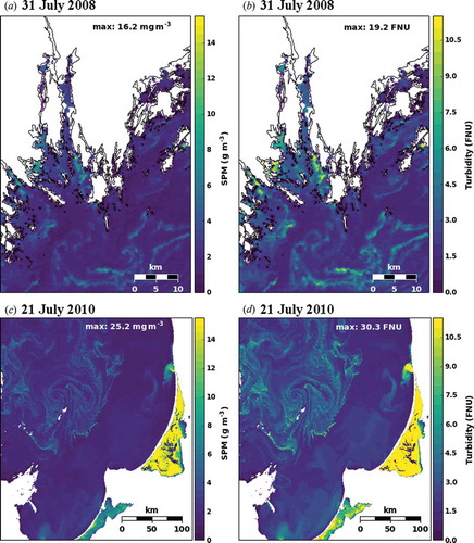
SPM concentrations from the MERIS standard SPM product were tested against the match-up dataset. The MNB was 11.3%, and the RMS was 47.4% for the Swedish coastal waters (Figure 4(a)). For Lithuanian coastal waters, the MNB was −1.5% and the RMS 29.5%, showing that the MERIS standard SPM product showed better agreement with in situ measurements in Lithuanian (Figure 4(b)) than in Swedish coastal waters. After combining the match-up datasets, the MNB was 4.6% and the RMS was 39.1%. The results show that the MERIS retrieved SPM concentrations works very well for both validation areas with a wide range of SPM concentrations with reasonable error estimates. The developed SPM model (Equation (1)) was therefore used to derive turbidity from SPM concentrations from MERIS reflectance. The quadrature sum of errors was 9.7% for the MNB and 50.4% for the RMS, which is very reasonable for a level 2 product of such optically complex waters strongly influenced by biological processes. Figure 5 illustrates SPM and turbidity over the measurement sites in both areas, upper row the Himmerfjärden area in NW Baltic Sea (a and b) and lower row the Lithuanian study area in the SE Baltic Sea (c and d). The selected images show cyanobacteria bloom events in both areas, the dates were 31 July 2008 (a and c) and 21 July 2010 (b and d).

Figure 4. Comparison of MERIS SPM standard product against in situ SPM (g m^–3) (a) in Swedish, and (b) in Lithuanian coastal waters MERIS full-resolution data (3 × 3 pixel matrix), processor: MEGS 8.1 (n = 67). Note the different scales on the y-axis. The dashed line shows the 1:1 relationship.

Figure 5. Spatial distribution of SPM retrieved from the MERIS standard SPM product (MEGS 8.1) (a, c) and turbidity retrieved from MEGS using the developed SPM model (b, d) in and around Himmerfjärden bay in Sweden (upper row) in the Lithuanian study area (lower row) during the dates 31 July 2008 and 21 July 2010.

4. Discussion

The developed SPM model to retrieve SPM from turbidity predicted SPM concentrations with good quality. To develop the SPM model, an in situ dataset of turbidity and SPM concentration was collected from five areas in the north-western Baltic proper and in the continuum river–lagoon–coastal zone of the Lithuanian coast (eastern Baltic proper). The measurement error of in situ SPM in this study was about 12% within the Swedish dataset and 11% within the Lithuanian dataset. The errors are similar to a previous study by Kratzer (2000), who calculated a standard error of about 10% for in situ SPM for the NW Baltic Sea. Errors in the SPM measurements can be introduced by both filter handling errors and by insufficient stirring of the sample. The sample should be stirred thoroughly before filtration to secure an even distribution of suspended material in the sampling bottle. Another cause of error may be introduced if the seawater sample is not rinsed with ultrapure water to avoid the formation of salt crystals on the filter (Neukermans et al. 2012). In addition, small particles may pass the filter, although usually the filter clogs rather quickly reducing the initial nominal pore size of 0.7 µm closer to a pore size of 0.2 µm. The measurement error of in situ turbidity was about 10%, within the Swedish dataset and 13% within the Lithuanian dataset. The measurement uncertainty for turbidity is approximately in the same range as for SPM measurements. Turbidity measurements do not require much training, which makes them more versatile. For example, they would be suited for citizen science or volunteer monitoring projects as the method is quite easy to learn and rather low cost. However, there are still some pitfalls with the method. Insufficient stirring of the sample, for example, may cause errors also in turbidity measurements. The measurement can also be influenced by faulty handling of the glass vial, for example, touching of the sides of the sampling vial.

The SPM model was tested on two independent validation datasets, from the Swedish coastal waters in the NW Baltic proper and from the Lithuanian coastal waters in the SE Baltic proper. The validation in the NW Baltic proper showed very good results (r = 0.99, MNB 2.4%, RMS 25%) and the values were placed quite tightly around the 1:1 line. When testing the SPM model on the dataset from the SE Baltic proper, we also got very good statistical values (r = 0.95, MNB 14%, RMS 37%). However, the comparison between SPM modelled and in situ SPM (Figure 3(b)) shows that more of the higher values lie above the 1:1 line. This may be related to multiple scatter. At high concentrations, it is more likely that the same photon is scattered more than once by a particle, leading to an overestimation of the actual SPM concentration. At lower concentrations, the values are more closely situated around the 1:1 line (both in Figure 3(a and b)), indicating that the particles are less likely to be submitted to multiple scatter. Note that some of the relative errors can also be attributed to patchiness in the water body which usually increases at high concentrations, and also due to measurement errors. However, there is no reason to believe that such phenomena should have a bias with regards to the 1:1 line as errors in handling or water patchiness are likely to be random. When combining the Swedish and Lithuanian datasets, the validation shows overall very good results (MNB = 9%, RMS = 32%) for the Baltic.

In the Lithuanian coast, of the SE Baltic Sea, the SPM concentration may exceptionally reach up to 32 g m⁻³ (median of 4.4 g m⁻³), when measured in the plume of the Curonian Lagoon (Vaičiūtė, Bresciani, and Bučas. 2012). In other areas of the Baltic Sea, such as the Vistula Lagoon, Gulf of Gdansk, Gulf of Riga, and Gulf of Finland, the in situ SPM concentrations range from 0.4–16.0, 10.0–24.2, 0.8–6.0, and 0.8–2.6 g m⁻³, respectively (Woźniak et al. 2011; Raag, Sipelgas, and Uiboupin 2014; Vazyulya et al. 2014; Koponen et al. 2007). Ohde, Siegel, and Gerth (2007) measured a range of 0.4–9.0 g m⁻³ in the Arkonian Sea, the Bornholm Sea, and the Gotland Sea. In the Pomeranian Bight, they found values up to 20 g m⁻³. In the Öre Estuary in the Bothnian Sea, Harvey, Kratzer, and Andersson (2015) found values between 0.2 and 20.9 g m⁻³. Kyryliuk and Kratzer (2016) derived SPM concentrations for different Baltic Sea basins from MERIS data processed with the coastal water processor using a neural network developed by the Free University Berlin (FUB) (Schroeder et al. 2007). The median values in each sub-basin lie very well within the range of the developed SPM model. The ranges of SPM found in the Baltic Sea are generally low relative to marine waters, indicating that the developed SPM model should be applicable for most of the Baltic Sea. However, shallow coastal lagoons, such as the Curonian Lagoon and the Vistula Lagoon in the SE Baltic Sea, in transition between land and the sea may have exceptionally high SPM concentrations exceeding 70 g m⁻³ during summer (unpublished data). Such extreme values mainly co-occur in conjunction with intensive algal blooms and are rather extreme and thus more of an exception in the Baltic Sea, rather than the rule. During other special events such as storms, strong run-off, or dredging, SPM concentrations may also exceed the limits of the model. Due to the selection of the turbidity measurement mode (see Section 2), the highest accuracy of the SPM model was up to SPM concentration of 16.9 g m⁻³ (which corresponds to 20 FNU). The SPM model needs to be applied with caution when the concentrations are beyond this value and hence the model may show higher errors. However, in the validation datasets the SPM model predicts also the higher values with good quality. In the Lithuanian dataset, the maximum in situ turbidity was 49.8 FNU (corresponding to modelled SPM 34 g m⁻³) and despite the high range of values, the correlation coefficient was very strong (r = 0.95) (Table 2). Therefore, the developed SPM model is reliable in the Baltic Sea, despite the relatively low SPM and high CDOM concentrations (Kratzer and Tett 2009; Kutser et al. 2009). CDOM absorption is highest in the visible short wavelengths (350–500 nm) and decreases exponentially with increasing wavelength (J. T. O. Kirk 2010). The North Sea has high particle scatter due to high tidal influence and therefore much higher SPM concentrations than the Baltic Sea. The bio-optical characteristics of the Baltic Sea, however, are optically dominated by CDOM absorption (Christiansen, Lund-Hansen, and Christiansen 2008; Kratzer 2000). In order to avoid the effect of CDOM absorption on turbidity measurements, in situ turbidity was measured according to the ISO 7027 method in the near-infrared (at 860 or 850 nm), where the CDOM absorption is negligible. The SPM model was compared with a regional in-water SPM model developed by Nechad, Ruddick, and Neukermans (2009) using MERIS data over the North Sea. The model is rather similar to the in-water SPM model developed in the current study, but it showed a clear off-set to Nechad’s model. This is presumably due to the different specific inherent optical properties of Baltic Sea particles, that is, the scatter to backscatter ratio as well as the volume scattering function.

Dogliotti et al. (2015) showed that a general single-band algorithm (using 645 and 859 nm bands) can be used to retrieve turbidity from water-leaving reflectance in various regions. As turbidity is a physical measure of scatter (at a 90° angle), it is related to backscatter, and hence also to remote sensing reflectance (Dogliotti et al. 2015). However, in this study there was no turbidity match-up data available. Hence, the MERIS standard SPM product was tested against the match-up SPM dataset instead. The correlation between MERIS-retrieved SPM and in situ SPM was very high for both areas, with r = 0.74 for the Swedish dataset and r = 0.94 for the Lithuanian dataset. The selection of in situ measurements within ±2 hours of the satellite overpass time improved the relationship between in situ SPM and standard MERIS level 2 SPM products (Beltrán-Abaunza, Kratzer, and Brockmann 2014). Vaičiūtė, Bresciani, and Bučas. (2012) tested the standard MERIS level 2 SPM products in the SE Baltic Sea earlier (from the previous, second reprocessing) for the MEGS, C2R, Eutrophic, Boreal, and FUB processors. However, the authors used the whole dataset available, without restricting match-ups to a time window of ±2 hours. The concentration of SPM was here predicted better with the FUB processor (r = 0.93) than with MEGS (r = 0.75). Beltrán-Abaunza, Kratzer, and Brockman (2014) showed that the retrieval of SPM worked best with the MERIS standard processor in the NW Baltic Sea when compared with the other processors developed for optically complex waters, with an MNB ranging from 8% to 16% and an RMSE of about 33–42%. For the validation dataset in this study, the MNB showed an overestimation of about 11% in Swedish coastal waters, whereas in Lithuanian coastal waters the SPM product showed only a very small MNB and a slight underestimation of −1.5%. The RMS of SPM retrieval was about 47% in Swedish and 30% in Lithuanian coastal waters. The bias is generally very low for a level 2 product in the Baltic Sea (Kratzer and Vinterhav 2010; Beltrán-Abaunza, Kratzer, and Brockmann 2014; Vaičiūtė, Bresciani, and Bučas. 2012). The bias in retrieving these optical properties by MERIS standard products is presumably caused by the fact that both the CDOM and chl-a absorption as well as SPM scattering are all derived from the remote sensing reflectance at 442 nm. Therefore, these components and their derived concentrations are linked to each other and if one of them is over- or underestimated, the retrieval of the other two components is affected. The standard processor MEGS is trained on a CDOM absorption (at 442 nm) range of 0.005–5.000 m⁻¹ and on an SPM concentration range of 0.5–50.0 g m⁻³, which should be adequate for Baltic Sea waters. However, in the Baltic Sea, CDOM absorption is known to be highly underestimated by all available MERIS processors (Kratzer and Vinterhav 2010; Beltrán-Abaunza, Kratzer, and Brockmann 2014).

In order to test whether it is possible to get an SPM concentration estimate based on single remote sensing reflectance, we tested the retrieval of turbidity from the MERIS reflectances band at 620 nm, according to Nechad, Ruddick, and Neukermans (2009). However, the retrieval of turbidity at near-infrared is not reliable if chl-a fluorescence is expected to have a significant effect (Nechad, Ruddick, and Neukermans 2009). After retrieving turbidity from remote sensing reflectance, the SPM model was applied to estimate SPM concentrations. The combination of Nechad’s turbidity algorithm and our SPM model predicted SPM concentrations with improved accuracy when compared with the MERIS standard SPM product in Swedish coastal sites, but the concentrations were highly underestimated at SPM values above 2.5 g m⁻³. In Lithuanian coastal waters, the assessment showed even stronger underestimation at high SPM concentrations and even stronger deviation from the 1:1 line, whereas the MERIS standard SPM product showed a low scatter around the 1:1 line and overall lower errors. In Figure 5, the MERIS images show the distribution of SPM and of turbidity retrieved from MERIS with the developed SPM model for both investigated regions in the Baltic Sea. For the retrieval, the original regression model had to be inverted (i.e. to retrieve turbidity from SPM instead) and was then applied to the MEGS-derived SPM product. Figure 5 shows the distributions of SPM (a and c) and turbidity (b and d), a gradient of decreasing values from coastal areas to open sea. The comparison illustrates that by applying the SPM model the distinction between the land-derived SPM and the off-shore SPM caused by cyanobacterial production can be improved, since the SPM concentrations are lower in the area between the bay and the off-shore bloom. In the Himmerfjärden area, the maximum SPM concentration was 16.2 g m⁻³ and the maximum retrieved turbidity was 19.2 FNU. Whereas at the Lithuanian sites, the maximum SPM and turbidity values were much higher with SPM concentration 25.2 g m⁻³ and turbidity 30.3 FNU. The maximum values measured in both areas are within the validation range of the model.

5. Conclusions

This study confirms that the SPM concentration in the Baltic Sea strongly correlates with in situ measured turbidity (ISO 7027) despite the high background CDOM absorption in this semi-enclosed brackish sea. The relationship between these two important environmental and optical variables remains relatively constant in spite of the large spatial and annual variation in SPM within the two investigated sub-regions of the Baltic Sea. The validation datasets were shown to be representative in terms of SPM concentration for the Baltic Sea in general, and thus the model can be applied regionally. The results also showed that MEGS can retrieve SPM very reliably from MERIS data when restricting the match-up window to ±2 hours, and by using the empirical relationship between SPM turbidity, we could also infer turbidity from MERIS data. The presented MERIS images exemplify how the spatial and temporal variability and distribution of algal blooms and sediments can be better understood using MERIS data. Therefore, we would like to recommend the use of remote sensing data for regular monitoring of the Baltic Sea, especially in coastal waters. Remote sensing has shown to improve the temporal and spatial resolution of monitoring data in the Baltic Sea (Kratzer, Harvey, and Philipson 2014; Harvey, Kratzer, and Philipson 2015). By combining our SPM model with remote sensing data the monitoring of suspended material can be made much more cost-effective. On 16 February 2016, the Ocean Colour Land Instrument (OLCI) instrument has been launched on the satellite platform Sentinel-3 as part of the operational Copernicus mission. OLCI will have capabilities similar to MERIS, but will be fitted with additional bands, for example, in the short-wave infrared (SWIR) at 1020 nm to improve atmospheric correction. This would allow reserving the channel at 860 nm for the retrieval of turbidity instead of using it for atmospheric correction. It must be noted, however, that 860 nm band is less sensitive to lower turbidity values (<30 FNU) than algorithms based on shorter wavelengths. Our evaluation showed that 620 nm reflectance can be used to retrieve low turbidity values of up to about 3 FNU. More work has to be done to investigate which reflectance channels could be used to derive turbidity in Baltic Sea waters with intermediate turbidity ranging between 3 and 30 FNU.

In this paper, a Baltic Sea–specific algorithm was used to derive turbidity from the MEGS SPM product rather than directly from reflectance data. It is likely that the same approach can also be applied to OLCI data as the operational SPM product for OLCI will be based on the same processor as evaluated here. The algorithm will be tested in the future with dedicated turbidity match-up data. Since turbidity is listed as a mandatory parameter in Annex III of the European Union’s Marine Strategy Framework Directive (European Commission 2008, Annex III), we also recommend regular turbidity measurements in monitoring programmes for the Baltic Sea.

Acknowledgements

Funding was provided by the Swedish National Space Board (SNSB, Dnr. 147/12), the European Space Agency (ESA, contract no. 21524/08/I-OL), by VR project 349-2011-2337, by NordForsk project 42041 and by the strategic project ‘Baltic Sea Adaptive Management’ (BEAM) (SU: 4315403). Part of the field sampling and the water quality data was sampled in collaboration with the Swedish Environmental Protection Agency project WATERS and Svealands Kustvattenvårdsförbund. Thanks to ESA and ACRI-ST for developing ODESA, available at http://earth.eo.esa.int/odesa. This study was co-funded by the European Community’s Seventh Framework Programme (FP7/2007-2013) under grant agreement no. 606865, INFORMS project and BONUS BIO-C3 project, supported by BONUS (Art 185), funded jointly by the EU and National Research Council of Lithuania (D. Vaičiūtė). Thanks to Andreas Hicketier and Ilias Thomas from Stockholm University (SU) for statistical help and to Jakob Walve (SU) and the marine monitoring group (SU) for collecting some of the in situ data. Great thanks to Askö Laboratory (SU) for providing research facilities. Thanks to Mariano Bresciani, Erica Matta, and Claudia Giardino from Optical Remote Sensing group, CNR-IREA, Italy, for the significant contribution during field campaign in July 2012. We also thank the two anonymous reviewers for very valuable comments that led to a clear improvement of this manuscript.

Disclosure statement

No potential conflict of interest was reported by the authors.

Additional information

Funding

Funding was provided by the Swedish National Space Board (SNSB, Dnr. 147/12), the European Space Agency (ESA, contract no. 21524/08/I-OL), by VR project 349-2011-2337, by NordForsk project 42041 and by the strategic project ‘Baltic Sea Adaptive Management’ (BEAM) (SU: 4315403). This study was co-funded by the European Community’s Seventh Framework Programme (FP7/2007-2013) under grant agreement no. 606865, INFORMS project and BONUS BIO-C3 project, supported by BONUS (Art 185), funded jointly by the EU and the National Research Council of Lithuania (D. Vaičiūtė).

References

- ACRI-ST. 2012. “ODESA Software Distribution. Quick Start Guide”. version 1.2.4. http://www.odesa-info.eu/distrib/doc/ODESA_QSG_v1.2.4.pdf.
- Arruda, J. A., G. Richard Marzolf, and R. T. Faulk. 1983. “The Role of Suspended Sediments in the Nutrition of Zooplankton in Turbid Reservoirs.” Ecology 64 (5): 1225–1235. doi:10.2307/1937831.
- Beltrán-Abaunza, J. M., S. Kratzer, and C. Brockmann. 2014. “Evaluation of MERIS Products from Baltic Sea Coastal Waters Rich in CDOM.” Ocean Science 10 (3): 377–396. doi:10.5194/os-10-377-2014.
- Binding, C. E., D. G. Bowers, and E. G. Mitchelson-Jacob. 2005. “Estimating Suspended Sediment Concentrations from Ocean Colour Measurements in Moderately Turbid Waters: The Impact of Variable Particle Scattering Properties.” Remote Sensing of Environment 94 (3): 373–383. doi:10.1016/j.rse.2004.11.002.
- Blaas, M., C. Dong, P. Marchesiello, J. C. McWilliams, and K. D. Stolzenbach. 2007. “Sediment-Transport Modeling on Southern Californian Shelves: A ROMS Case Study.” Continental Shelf Research 27 (6): 832–853. doi:10.1016/j.csr.2006.12.003.
- Bourg, L., and Members of the MERIS Quality Working Group. 2011. “MERIS 3rd Data Reprocessing. Software and ADF Updates“. Report no. A879.NT.008.ACRI-ST, ACRI-ST, June 27.
- Bowers, D. G., and C. E. Binding. 2006. “The Optical Properties of Mineral Suspended Particles: A Review and Synthesis.” Estuarine Coastal and Shelf Science 67 (1–2): 219–230. doi:10.1016/j.ecss.2005.11.010.
- Bukata, R. P., J. H. Jerome, K. Ya, Kondratyev, and D. V. Pozdnyakov. 1995. Optical Properties and Remote Sensing of Inland and Coastal Waters. Boca Raton, FL: CRC Press, Inc.
- Christiansen, C., L. C. Lund-Hansen, and C. Christiansen. 2008. “Suspended Particulate Matter (SPM) in the North Sea-Baltic Sea Transition: Distributions, Inventories, and the Autumn 2002 Inflows.” Geografisk Tidsskrift-Danish Journal of Geography 108 (2): 37–47. doi:10.1080/00167223.2008.10649587.
- Dailidienė, I., and L. Davulienė. 2008. “Salinity Trend and Variation in the Baltic Sea near the Lithuanian Coast and in the Curonian Lagoon in 1984–2005.” Journal of Marine Systems 74 (Dec.): S20–S29. doi:10.1016/j.jmarsys.2008.01.014.
- Davies-Colley, R. J., and D. G. Smith. 2001. “Turbidity, Suspended Sediment and Water Clarity: A Review.” Journal of the American Water Resources Association 37 (5): 1085–1101. doi:10.1111/j.1752-1688.2001.tb03624.x.
- Doerffer, R. 2002. “Protocols for the Validation of MERIS Water Products – PO-TN-MEL-GS-0043.” ESA Publication PO-TN-MEL-GS-0043, no. 1. https://earth.esa.int/workshops/mavt_2003/MAVT-2003_801_MERIS-protocols_issue1.3.5.pdf.
- Doerffer, R., and H. Schiller. 2007. “The MERIS Case 2 Water Algorithm.” International Journal of Remote Sensing 28 (3–4): 517–535. doi:10.1080/01431160600821127.
- Dogliotti, A. I., K. G. Ruddick, B. Nechad, D. Doxaran, and E. Knaeps. 2015. “A Single Algorithm to Retrieve Turbidity from Remotely-Sensed Data in All Coastal and Estuarine Waters.” Remote Sensing of Environment 156 (Jan.): 157–168. doi:10.1016/j.rse.2014.09.020.
- European Commission. 2008. “Directive 2008/56/EC of the European Parliament and of the Council, of 17 June 2008, Establising a Framework for Community Action in the Field of Marine Environmental Policy (Marine Strategy Framework Directive).” Official Journal of the European Communities L164/1: 164/19–164/40.
- Ferrarin, C., A. Razinkovas, S. Gulbinskas, G. Umgiesser, L. Bliūdžiutė. 2008. “Hydraulic Regime-Based Zonation Scheme of the Curonian Lagoon.” Hydrobiologia 611 (1): 133–146. doi:10.1007/s10750-008-9454-5.
- Fettweis, M., and D. Van den Eynde. 2003. “The Mud Deposits and the High Turbidity in the Belgian–Dutch Coastal Zone, Southern Bight of the North Sea.” Continental Shelf Research 23 (7): 669–691. doi:10.1016/S0278-4343(03)00027-X.
- Fleming, V., and S. Kaitala. 2006. “Phytoplankton Spring Bloom Intensity Index for the Baltic Sea Estimated for the Years 1992 to 2004.” Hydrobiologia 554 (1): 57–65. doi:10.1007/s10750-005-1006-7.
- Form, C. C., I. Borsenkova, O. B. Christensen, J. Elken, J. Haapala, B. Hünicke, J. Käyhkö, et al. 2004. “The Baltic Sea.” Remote Sensing of Environment 30(1). Elsevier Oceanography Series. doi:10.1007/s10750-005-1006-7.
- Harvey, E. T., S. Kratzer, and P. Philipson. 2015. “Satellite-Based Water Quality Monitoring for Improved Spatial and Temporal Retrieval of Chlorophyll-a in Coastal Waters.” Remote Sensing of Environment 158: 417–430. doi:10.1016/j.rse.2014.11.017.
- Harvey, E. T., S. Kratzer, and A. Andersson. 2015. “Relationships between Colored Dissolved Organic Matter and Dissolved Organic Carbon in Different Coastal Gradients of the Baltic Sea.” AMBIO 44 (S3): 392–401. doi:10.1007/s13280-015-0658-4.
- HELCOM. 2014. “ Manual for Marine Monitoring in the COMBINE Programme of HELCOM.” Annex C-4 Phytoplankton chlorophyll-a. http://www.helcom.fi/Documents/Action%20areas/Monitoring%20and%20assessment/Manuals%20and%20Guidelines/Manual%20for%20Marine%20Monitoring%20in%20the%20COMBINE%20Programme%20of%20HELCOM_PartC_AnnexC4.pdf
- Hicketier, A., and I. Thomas. 2015. Consulting Report: SPM-Turbidity Case. Stockholm: Department of Mathematical Statistics, Stockholm University.
- Jassby, A. D., J. E. Cloern, and B. E. Cole. 2002. “Annual Primary Production: Patterns and Mechanisms of Change in a Nutrient-Rich Tidal Ecosystem.” Limnology and Oceanography 47 (3): 698–712. doi:10.4319/lo.2002.47.3.0698.
- Jeffrey, S. W., and M. Vesk. 1997. Introduction to Marine Phytoplankton and Their Pigment Signatures. In Phytoplankton Pigments in Oceanography: Guidelines to Modern Methods. Paris: UNESCO Publishing.
- Jerlov, N. 1976. Marine Optics. J. Mar. Biol. Ass, xii, 231. Elsevier Oceanography Series, 14). Vol. 58. Cambridge University Press (CUP); Elsevier Scientific Publishing Company. doi:10.1017/s0025315400028277.
- Kallio, K. 2012. “Water Quality Estimation by Optical Remote Sensing in Boreal Lakes.” PhD thesis, University of Helsinki, Helsinki.
- Kirk, J. T. O. 2010. Light and Photosynthesis in Aquatic Ecosystems. 3rd ed. Cambridge University Press. doi:10.1017/CBO9781139168212.
- Kirk, K. L., and J. J. Gilbert. 1990. “Suspended Clay and the Population Dynamics of Planktonic Rotifers and Cladocerans.” Ecology 71 (5): 1741–1755. doi:10.2307/1937582.
- Koponen, S., J. Attila, J. Pulliainen, K. Kallio, T. Pyhälahti, A. Lindfors, K. Rasmus, and M. Hallikainen. 2007. “A Case Study of Airborne and Satellite Remote Sensing of a Spring Bloom Event in the Gulf of Finland.” Continental Shelf Research 27: 228–244. doi:10.1016/j.csr.2006.10.006.
- Kowalczuk, P., C. A. Stedmon, and S. Markager. 2006. “Modeling Absorption by CDOM in the Baltic Sea from Season, Salinity and Chlorophyll.” Marine Chemistry 101 (1–2): 1–11. doi:10.1016/j.marchem.2005.12.005.
- Kratzer, S. 2000. “Bio-Optical Studies of Coastal Waters.” PhD Thesis, University of Wales, Bangor.
- Kratzer, S., and P. Tett. 2009. “Using Bio-Optics to Investigate the Extent of Coastal Waters: A Swedish Case Study.” Eutrophication in Coastal Ecosystems: 169–186. doi:10.1007/978-90-481-3385-7_15.
- Kratzer, S., and C. Vinterhav. 2010. “Improvement of MERIS Level 2 Products in Baltic Sea Coastal Areas by Applying the Improved Contrast between Ocean and Land Processor (ICOL) – Data Analysis and Validation.” Oceanologia 52 (2): 211–236. doi:10.5697/oc.52-2.211.
- Kratzer, S., E. T. Harvey, and P. Philipson. 2014. “The Use of Ocean Color Remote Sensing in Integrated Coastal Zone Management-A Case Study from Himmerfjärden, Sweden.” Marine Policy 43: 29–39. doi:10.1016/j.marpol.2013.03.023.
- Kutser, T., B. Paavel, L. Metsamaa, and E. Vahtmäe. 2009. “Mapping Coloured Dissolved Organic Matter Concentration in Coastal Waters.” International Journal of Remote Sensing 30 (22): 5843–5849. doi:10.1080/01431160902744837.
- Kyryliuk, D., and S. Kratzer. 2016. “Total Suspended Matter Derived from MERIS Data as Indicator for Coastal Processes in the Baltic Sea; Manuscript Submitted to Ocean Sciences (Os-2016-2).” Ocean Science Discussions: 1–30. doi:10.5194/os-2016-2.
- Lindström, M., L. Håkanson, O. Abrahamsson, and H. Johansson. 1999. “An Empirical Model for Prediction of Lake Water Suspended Particulate Matter.” Ecological Modelling 121 (2–3): 185–198. doi:10.1016/s0304-3800(99)00081-2.
- Lithner, G., K. Holm, and C. Ekström 2003. “Metaller Och Organiska Miljögifter I Vattenlevande Organismer Och Deras Miljö I Stockholm 2001. Metals and Organic Environmental Toxins in Aquatic Organisms and Their Environments within Stockholm Area 2001.” ITM Rapport Nt. 108. ISBN91-631-3785-5.
- Lucas, L. V., J. R. Koseff, J. E. Cloern, S. G. Monismith, and J. K. Thompson. 1999. “Processes Governing Phytoplankton Blooms in Estuaries. I: The Local Production-Loss Balance.” Marine Ecology Progress Series 187: 1–15. doi:10.3354/meps187001.
- Lunt, J., and D. L. Smee. 2014. “Turbidity Influences Trophic Interactions in Estuaries.” Limnology and Oceanography 59 (6): 2002–2012. doi:10.4319/lo.2014.59.6.2002.
- MacKenzie, B. R., and T. KiØrboe. 2000. “Larval Fish Feeding and Turbulence: A Case for the Downside.” Limnology and Oceanography 45 (1): 1–10. doi:10.4319/lo.2000.45.1.0001.
- Malmaeus, J. M., and L. Håkanson. 2003. “A Dynamic Model to Predict Suspended Particulate Matter in Lakes.” Ecological Modelling 167 (3): 247–262. doi:10.1016/s0304-3800(03)00166-2.
- Miller, R. L., and B. A. McKee. 2004. “Using MODIS Terra 250 M Imagery to Map Concentrations of Total Suspended Matter in Coastal Waters.” Remote Sensing of Environment 93 (1–2): 259–266. doi:10.1016/j.rse.2004.07.012.
- Nechad, B., K. G. Ruddick, and G. Neukermans. 2009. “Calibration and Validation of a Generic Multisensor Algorithm for Mapping of Turbidity in Coastal Waters.” Proceedings of SPIE 7473: 74730H–74730H–12. doi:10.1117/12.830700.
- Nechad, B., K. G. G. Ruddick, and Y. Park. 2010. “Calibration and Validation of a Generic Multisensor Algorithm for Mapping of Total Suspended Matter in Turbid Waters.” Remote Sensing of Environment 114 (4): 854–866. doi:10.1016/j.rse.2009.11.022.
- Neukermans, G., K. Ruddick, H. Loisel, and P. Roose. 2012. “Optimization and Quality Control of Suspended Particulate Matter Concentration Measurement Using Turbidity Measurements.” Limnology and Oceanography: Methods 10: 1011–1023. doi:10.4319/lom.2012.10.1011.
- Ohde, T., H. Siegel, and M. Gerth. 2007. “Validation of MERIS Level-2 Products in the Baltic Sea, the Namibian Coastal Area and the Atlantic Ocean.” International Journal of Remote Sensing 28 (3–4): 609–624. doi:10.1080/01431160600972961.
- Raag, L., L. Sipelgas, and R. Uiboupin. 2014. “Analysis of Natural Background and Dredging-Induced Changes in TSM Concentration from MERIS Images near Commercial Harbours in the Estonian Coastal Sea.” International Journal of Remote Sensing 35 (18): 6764–6780. doi:10.1080/01431161.2014.963898.
- Ruddick, K., B. Nechad, G. Neukermans, Y. Park, and D. Doxaran. 2008. “Remote Sensing of Suspended Particulate Matter in Turbid Waters: State of the Art and Future Perspectives.” Proceedings of the Ocean Optics XIX Conference, Barga (Italy), October 6–10. http://www2.mumm.ac.be/downloads/publications/ruddick_oceanoptics_2008.pdf.
- Salonen, M., and J. Engström-Öst. 2013. “Growth of Pike Larvae: Effects of Prey Turbidity and Food Quality.” Hydrobiologia 717 (1): 169–175. doi:10.1007/s10750-013-1575-9.
- Schroeder, T., I. Behnert, M. Schaale, J. Fischer, and R. Doerffer. 2007. “Atmospheric Correction Algorithm for MERIS above case-2 Waters.” International Journal of Remote Sensing 28 (7): 1469–1486. doi:10.1080/01431160600962574.
- Strickland, J. D. H., and T. R. Parsons. 1972. A Practical Handbook of Seawater Analysis. Ottawa: Fisheries Research Board of Canada Series.
- Suursaar, Ü., T. Kutser, R. Aps, T. Kullas, E. Vahtmäe, L. Metsamaa, and M. Otsmann. 2009. “Hydrodynamically Induced or Modified Patterns Derived from Satellite Images in the Coastal Waters of Estonia.” Journal of Coastal Research 2: 1602.
- Vaičiūtė, D., M. Bresciani, and M. Bučas. 2012. “Validation of MERIS Bio-Optical Products with in Situ Data in the Turbid Lithuanian Baltic Sea Coastal Waters.” Journal of Applied Remote Sensing 6 (1): 63520–63568. doi:10.1117/1.JRS.6.063568.
- Vazyulya, S., A. Khrapko, O. Kopelevich, V. Burenkov, T. Eremina, and A. Isaev. 2014. “Regional Algorithms for the Estimation of Chlorophyll and Suspended Matter Concentration in the Gulf of Finland from MODIS-Aqua Satellite Data.” Oceanologia 56 (4): 737–756. doi:10.5697/oc.56-4.737.
- Woźniak, S. B., J. Meler, B. Lednicka, A. Zdun, and J. Sto’n-Egiert. 2011. “Inherent Optical Properties of Suspended Particulate Matter in the Southern Baltic Sea.” Oceanologia 53 (3): 691–729. doi:10.5697/oc.53-3.691.