Improved forest-cover mapping based on MODIS time series and landscape stratification

ABSTRACT

Detailed forest-cover mapping at a regional scale by supervised classification is technically limited by various factors. This study evaluates the ability of a landscape stratification method to improve classification accuracy. An object-based segmentation technique (OBIA) was performed to delineate radiometrically homogeneous regions into the study area, used as strata for the classification of a time series of Moderate Resolution Imaging Spectroradiometer (MODIS) normalized difference vegetation index (NDVI) data. As a reduction of the spatial variability of the signatures of the vegetation classes is expected, Maximum Likelihood Classifier (MLC) was used to analyse potential effects on classification accuracy. Accuracy assessment was based on the calculation of kappa coefficient (κ) and reject fraction (RF). The values obtained with and without stratification were compared, to assess their global and per-stratum influence on the quality of a detailed forest-cover map (20 different classes). To study the influence of topographical and landscape stratum characteristics on classification accuracy, eight indicators were calculated. Their correlation with κ and RF differences due to stratification was analysed. Our study showed that stratification improved global and per-stratum classification accuracy and in parallel caused an RF increase. Both these evolutions are not conditioned by the stratum topographical and landscape characteristics but strongly influenced by stratum and classified vegetation area.

1. Introduction

Producing forest-cover maps characterized by both a detailed forest-type nomenclature and a sufficient accuracy is still difficult because of technical limitations related to supervised classification (Stehman et al. 2011; Kuemmerle et al. 2006).

Image classification using spectral signature allows land-cover mapping. However, focusing on forest mapping only broad vegetation categories are usually classified: forest and non-forest, forest and shrubland, or broadleaf and needleleaf, but most often forest resource information as species or forest types are not distinguished (Xie, Sha, and Yu 2008; Boyd and Danson 2005; Evans and Geerken 2006; Dymond, Mladenoff, and Radeloff 2002; Carrão, Gonçalves, and Caetano 2007; Redo and Millington 2011). The temporal signature is utilized to improve the recognition of different forest or natural vegetation types. It is based on the variability of their spectral response over time, linked to their phenological behaviour (Xie, Sha, and Yu 2008; Pettorelli et al. 2005; Clark et al. 2010). The corresponding temporal signatures are often extracted from vegetation index images and they qualify the seasonal or annual species behaviour. Their values can be related to the canopy photosynthetic capacity. The normalized difference vegetation index (NDVI) (Tucker and Sellers 1986; Pettorelli et al. 2005; Rouse et al. 1973) is commonly used to map vegetation with a temporal approach (Tucker and Sellers 1986; DeFries, Hansen, and Townshend 1995). Such an approach requires image acquisition at a regular and short time step. High temporal resolution sensors such as Système Probatoire d’Observation de la Terre (SPOT_Vegetation), National Oceanic and Atmospheric Administration-Advanced Very High Resolution Radiometer (NOAA-AVHRR), Environment Satellite-Medium Resolution Imaging Spectrometer (ENVISAT-MERIS), and Terra-Moderate Resolution Imaging Spectroradiometer (Terra-MODIS) supply such data usually with a daily temporal resolution (Xie, Sha, and Yu 2008; Ganguly et al. 2010; Friedl et al. 2002, 2010; García-Mora, Mas, and Hinkley 2012). The spatial resolution of these images varies from 250 m to 1 km.

Forest-cover and natural vegetation mapping is commonly carried out from a temporal approach based on MODIS data (Hüttich et al. 2009; Carrão, Gonçalves, and Caetano 2008). In most cases, the maps result in only a distinction among deciduous forests, evergreen forests, and mixed forests (Xie, Sha, and Yu 2008). This technical limitation is due to various factors. The first one is due to the coarse spatial resolution of the images. In heterogeneous or fragmented landscapes, a single pixel can cover several forest types and hence can hardly be assigned to a single class (Sulla-Menashe et al. 2011). This can result, if the nomenclature is not suited, in a loss of accuracy (Foody et al. 1997; Broich et al. 2009; Giri et al. 2013). The second difficulty is linked to the capacity to distinguish between species with similar spectral and temporal signatures. Differentiating similar forest types, such as pines, or evergreen oaks, remains difficult. Finally, it was found that signatures of a given species could vary substantially between two distant locations. Indeed, when dealing with large areas, the spatial variability of environmental conditions can lead to a local modification of the plants’ development and of their phenological behaviour. The signatures are then less representative of the forest or vegetation classes, leading to classification errors (Cihlar 2000; Colditz et al. 2011; Justice, Holben, and Gwynne 1986; Krishna Prasad, Badarinath, and Eaturu 2007; Zhou et al. 2003; Nagendra 2001). These difficulties are strengthened in mountainous areas, where elevation and exposure variations create changing bioclimatic conditions, increasing the complexity and variability of the spatial distribution of the vegetation and of its phenology (Balthazar, Vanacker, and Lambin 2012; Colditz et al. 2011; Ren et al. 2009; Kuemmerle et al. 2006; Cihlar 2000; Blesius and Weirich 2005).

To address this issue, a common process is to stratify the study area into subregions (Cai et al. 2011; Stehman 2009). The purpose of the stratification is to reduce class signature heterogeneity, minimize intra-class variability, and maximize inter-class separability (Gertner et al. 2007; Delincé 2001; Stehman et al. 2011; Gallego and Stibig 2013). It has been widely used to improve the accuracy of image classification (Homer et al. 1997; Lillesand 1996; Pettinger 1982). With the use of stratification, a 10–15% improvement of the overall accuracy is expected (Bauer et al. 1994). Regular grid or administrative units can be efficiently used to define strata. This approach is useful when class signature heterogeneity is mainly related to linear distance. However, bioclimatic conditions and landscape are often more complex, and the simplest approaches show limits in the expected gain of accuracy (Homer and Galant 2001; Homer et al. 2004). From a mapping point of view, strata limits have to be consistent with landscape units to limit edge-matching inconsistencies. A wide and heterogeneous territory is thus commonly partitioned in bioclimatic zones (Reese et al. 2002; Homer et al. 2004). The strata are delineated according to landscape, soil, vegetation, and climatic conditions homogeneity (Stehman et al. 2011; Broich et al. 2009; Congalton 1991; Homer et al. 2004). This process is suitable to map forest cover, where spatial distribution largely depends on these factors (Cai et al. 2011). Delineation of strata can be based on existing maps and is primarily dependent on the availability of the required thematic data (Reese et al. 2002). An expert knowledge-based approach is often necessary to adjust the limits of the existing maps to the images content (Reese et al. 2002). The implementation of such a stratification then appears complicated, takes long to set up, and, in any case, difficult to transpose to another territory.

In a previous study, a method using an object-based image analysis (OBIA) was developed to delineate radiometrically homogeneous regions considered as landscape units (Bisquert, Bégué, and Deshayes 2015). This approach can be considered a more objective and reproducible method of stratification. OBIA was defined as ‘a sub-discipline of Geographic Information Science devoted to portioning remote-sensing imagery into meaningful image-objects, and assessing their characteristics through spatial, spectral and temporal scale’ (Hay and Castilla 2006). OBIA is developed on concepts such as segmentation, edge-detection, feature extraction, and classification (Blaschke 2010). The key stage consists in performing a segmentation procedure defined by one or more criteria of homogeneity. The segments are considered homogeneous regions and can be characterized by spectral and textural information (Otukei and Blaschke 2010). OBIA has been widely used with high and very high spatial resolution images, being especially useful when the objects of interest are composed of several pixels (Blaschke et al. 2014), for example, for classifying trees in images with sub-metric spatial resolution. The application of OBIA to coarse-resolution images is less common and presents more complications, especially in the evaluation of the results when frequently no reference data exists. However, a number of studies were carried out with MODIS data (Tsaneva, Krezhova, and Yanev 2010; Vintrou et al. 2012). In a previous work, OBIA was applied to coarse spatial resolution MODIS images for landscape mapping of the whole French country (Bisquert, Bégué, and Deshayes 2015).

The use of these homogeneous landscape units (HLUs) as stratification is an innovative approach, hereafter applied at the regional scale in a mountainous area. This approach is integrated as an improvement process of the forest-cover mapping of a large mountainous area, performed using supervised classification, based on a time series of MODIS images. Our work aims to consider the resulting radiometrically homogeneous units as landscape stratification units and incorporates them in the supervised classification procedure of a MODIS images time series. Considering such stratification at a regional scale contributes to restraining the spatial variability of the forest classes’ signatures. The objective is to assess the ability of this data to improve classification accuracy. For this purpose, the mapping results achieved with and without stratification are compared. To define useful criteria expressing the ability of a stratification to improve classification, the effects of the topographical and landscape features of the strata on classification accuracy were also studied.

2. Materials and methods

2.1. Study area

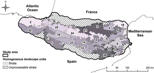
The study area is a mountain range (the Pyrenees) located at the border of France, Spain, and Andorra (Figure 1), covering a 50,000 km² area and spread over 400 km from the Atlantic Ocean to the Mediterranean Sea. The elevation varies from 200 m to over 3000 m. The general orientation of the range creates an East–West thermal gradient. A temperate oceanic climate is observed at the West, with mild and rainy winters and cool wet summers, thus following a cold sub-oceanic climate in the centre and a Mediterranean climate in the East, with mild winters and hot, dry summers (Soubeyroux et al. 2011).

Figure 1. Study area.

The precipitation amount is characterized by an important contrast, the annual average ranging from 1200 mm to 2400 mm. These altitudinal and climatic gradients determine varied ecological conditions. The forest vegetation of the study area presents a great diversity as well as a complex spatial distribution (Alcaraz-Segura, Paruelo, and Cabello 2006). The dominant tree species are beech (Fagus sylvatica), pine (Pinus sylvestris, Pinus uncinata, Pinus nigra), green oak (Quercus ilex), and different deciduous species. Numerous mixed types have been noted, particularly mixed forests of silver fir and beech (Daubet, De Miguel Magaña, and Maurette 2007), of mixed deciduous or evergreen oaks, and matoral areas.

2.2. Data

2.2.1. Images

MOD13Q1 products of Terra-MODIS were used for this study: 16 day composite images at 250 m spatial resolution with 23 syntheses available per year. In this product, NDVI (Rouse et al. 1973) and enhanced vegetation index (EVI) (Huete et al. 2002) are processed, and both vegetation indices were used in this study. Data set preprocessing included clipping the images to fit the study area, re-projecting them into the French geodesic system, cloud masking using quality data, and data errors correction using the adaptive Savitzky–Golay algorithm with TIMESAT Software (Jönsson and Eklundh 2004). Images were processed for the 2007–2011 period, short and recent enough to avoid long-term interactions but long enough not to be influenced by the climatic conditions of a particular year. In compliance with the OBIA methodology used (Bisquert, Bégué, and Deshayes 2015), the stratification process used EVI images. The original 16 day composites were processed to create monthly synthesis. Then, for each month, the five years (2007–2011) were averaged to produce a time series of 12 monthly average EVI images.

The supervised classification process used both NDVI and EVI images. In our classification improvement process based on a phenological approach, vegetation indices were identified as the most suitable phenological monitoring indicators to compose the temporal signature (Pettorelli et al. 2005). Images acquired in winter (December, January, February) were left out. Two periods of 3 years (2007–2009 and 2009–2011) were defined, to compare their results and establish that the values analysed are not period dependent. The three years were averaged to produce two time series of 16 day average NDVI composites, each one with 17 images.

2.2.2. Forest maps

A mapping database was created for the entire study area from national forest inventories, namely the ‘Inventaire Forestier National’ (IFN, http://inventaire-forestier.ign.fr/spip/) for France, the ‘Mapa Forestal de España’ (MFE, http://www.magrama.gob.es/es/biodiversidad/servicios/banco-datos-naturaleza/informacion-disponible/mfe50.aspx) for Spain, and the ‘Mapa Forestal del Principat d’Andorra’ (MFPA, http://www.iea.ad/mapa-forestal-del-principat-d-andorra) for Andorra. The different nomenclatures collected were harmonized. A final forest-type nomenclature was created from this database, composed of 18 mixed or mono-species forest types. It also includes four natural vegetation types, corresponding to alpine and mountain heathland and grassland (Table 1).

Table 1. Forest map nomenclature.

Class	Vegetation type
Deciduous oaks	Broadleaf forest
Mixed deciduous forest
Mixed mountain deciduous forest
Beech
Pyrenean oak
Holm oak
Evergreen oaks
Mountain pine	Coniferous forest
Aleppo pine
Pyrenean pine
Scots pine
Monterey pine
Silver fir
Beech and silver fir	Mixed broadleaf /coniferous forest
Wooded garrigue	Shrubland
Unwooded garrigue
Spanish matorral
Mountain Spanish matorral
Grassland	Heathland and grassland
Mountain heathland
Alpine heathland
Alpine grassland
Bare soil, rocks	-
Water	-

To assess the problem of scale difference between the forest map and coarse-resolution images, and to limit the edge effects, we chose to process only the pixels completely included in the polygons of the forest map. They cover about 25% of the study area. The gridded forest map of these fully included pixels was used for training and accuracy assessment in the classification process.

2.2.3. Land-use data

The Corine Land Cover (year 2006) database was used to carry out a statistical evaluation of the delineation of the HLUs obtained with OBIA analysis (http://www.eea.europa.eu/data-and-maps/data/corine-land-cover-2006-raster-3).

2.2.4. Digital elevation model

The digital elevation model (DEM) has been used as an ancillary data for supervised classification and OBIA analysis. It was extracted from the Shuttle Radar Topography Mission (SRTM) database. A version corrected by the Consortium for Spatial Information (CGIAR-CSI)  was used to create the elevation plan (Jarvis et al. 2008). A change of the spatial resolution from 90 m to 250 m was performed from the initial data, averaging the elevation values.

2.3. Method

2.3.1. HLUs delineation

The first step is to delineate HLUs using an existing object segmentation method . This method was applied to delimitate HLU fitted to our study area. The process consists in identifying the best combination of satellite-derived variables (spectral, textural, and temporal) and the best image segmentation parameters. The method was applied using a time series of monthly EVI average values calculated over the 2007–2011 period, and Haralick textural indices (Bauer et al. 1994), calculated on this series of images, with the ENVI software (Exelis Visual Information Solutions, Boulder, Colorado). The five indices are homogeneity, contrast, dissimilarity, entropy, and second moment. A 5 × 5 pixel window was used for their calculation. OBIA was applied with the ECognition software (Trimble, München, Germany). Two optimization steps were performed beforehand.

The first stage aims to decrease the number of variables composing the segmentation input data, initially 72 images: 12 EVI images + (12 × 5) texture images. Therefore, two successive principal component analyses (PCAs) were applied with the FactoMine R software (Lê, Josse, and Husson 2008). The first analysis was applied to all monthly images of each index (EVI and textural index), in order to identify the most representative dates. The three most representative dates were thus selected. Then, for each chosen date, a second PCA was applied to all the images (EVI or textural index), to analyse the correlation between them and to select the most representative images.

The second optimization stage aims to choose the best EVI/textural index combination and to optimize the segmentation parameters. This optimization is related to the homogeneity criteria, which has a direct influence on the HLU delineation. It is expressed by the scale parameter, which defines the maximal allowable heterogeneity threshold and therefore determines the size of the obtained segments. Different segmentations were performed, based on different EVI and textural indices combinations: EVI + homogeneity, EVI + entropy, EVI + secondary moment, EVI + contrast, and EVI + dissimilarity. As indicated in the original method, scale parameter values increasing from 5 to 50 were tested to perform the segmentation (Bisquert, Bégué, and Deshayes 2015).

The best combination and optimal scale parameters were chosen with two unsupervised evaluation methods of these segmentations, the respective methods of Zhang (Zhang, Xiao, and Feng 2012) and of Johnson (Johnson and Xie 2011). The Zhang method consists in analysing the inter-segment dissimilarity by comparing each segment to the global image. The Johnson method corresponds to a complementary approach and consists in evaluating the dissimilarity by comparing between joined segments. Each segmentation was therefore evaluated by calculating two statistical indices, respectively, named the Z and J indices (Bisquert, Bégué, and Deshayes 2015). For each of the five studied combinations, by varying the scale parameter from 5 to 50, two distinct assessment curves were obtained. The choice of the best EVI/textural index combination was based on the shape of the curves. For an appropriate segmentation, two curves, slowly decreasing to a minimum that corresponds to the optimal scale parameter, and then increasing, must be obtained. The two Z and J index curves must show those evolutions simultaneously. In the end, the textural index for which the two curves correspond to an optimal theoretical shape is selected and the optimum value of the scale parameter corresponds to their minimum. The HLU delineation in the study area is then carried out by an object segmentation based on those variables and parameters.

2.3.2. Strata definition and characterization

Strata definition: The HLU obtained by segmentation corresponds to the strata needed to clip the study area in this classification improvement approach. A preliminary step was needed to ensure that the strata obtained are adapted to this work. A first classification trial was performed with them, which showed that for some strata, the classification process could not be applied. These strata, called ‘unprocessable strata’, had a very small forest-cover area with at least one vegetation class presenting an insufficient amount of training pixels. The choice was made to merge those ‘critical strata’ with contiguous strata in order to increase the forest area and the class pixels amounts for the training data set. The fusion criterion was the land-cover similarity. To evaluate this criterion, the Corine Land Cover database (2006) was used. After extracting the different portions of land-cover classes, a Spearman correlation value (Spearman 1904) was calculated for each pair of contiguous strata. It was defined that a ‘critical stratum’ could merge with its adjacent stratum when its correlation value was higher than +0.9. The strata not meeting this criterion could not merge and therefore could not be mapped.

Computation of strata topographical and landscape indices: The obtained strata were characterized with a set of topographical or landscape indices. The eight selected indices are often used in landscape ecology (Forman and Godron 1986; Turner 1989). They were calculated for each stratum from the DEM or from the forest reference data. They are distributed into three categories (Table 2). Topographical indices report the stratum area and the more or less mountainous and uneven landform nature, which has a direct influence on the spatial composition and organization of vegetation. Area and spatial organization indices characterize the extent of the stratum forest cover and the diversity of the forest-cover patches. Several indices are based on patches. From an ecological perspective, patches are communities or species assemblages surrounded by a matrix with a dissimilar community structure or composition (Forman and Godron 1981). They represent areas of relatively homogeneous environmental conditions where the patch boundaries are distinguished by discontinuities in environmental character states from their surroundings. For this study, a patch was considered as a set of contiguous pixels from the same type. The indices relating to the patches area can also be considered as indicators of land fragmentation. Composition indices, including the Shannon index (Shannon 1948), characterize the diversity of the forest types composing the stratum forest cover.

Table 2. Indices describing the topographical and landscape characteristics of the strata.

Index	Description	Equation
Topographical indices
Area (ha)	Area of a stratum	AS: Stratum area (ha)
Elevation (standard deviation) (m)	Standard deviation of elevation values into a stratum	(1) eij: elevation (m) into the stratum E: Sum of the elevation values (m) into the stratum n: Number of elevation values for the stratum
Slope (average) (°)	Average slope value into a stratum
Area-derived and spatial organization landscape indices
Total forest-cover rate (%)	Total forest-cover rate for a stratum	AF: Total forest-cover area (m^2) AS: Stratum area (m^2)
Patch area (average) (ha)	Patch area average for a stratum	AS: Stratum area (m^2) n: Number of patches
Patch area (standard deviation) (ha)	Patch area standard deviation for a stratum	aij: IJ patch area (m^2) AS: Stratum area (m^2) n: Number of patches
Composition landscape indices
Number of classes	Number of classes for each stratum	-
Shannon Diversity index	Index indicating the class area rate of dispersion for a stratum	(5) Pi: Rate between a class area and the total area of all the classes

2.3.3. Supervised classification

The study area was mapped with a per-pixel supervised classification approach. The NDVI and EVI time series of the 2007–2009 and 2009–2011 periods were classified without stratification. Then, for each series, an independent classification was processed for each stratum and the results were merged for accuracy assessment. Because of its robustness, the Maximum Likelihood Classifier (MLC) classification algorithm was used for this process. All processing operations were performed with the ArcGis10 software (ESRI, Redlands, CA).

2.3.4. Accuracy assessment

The training data set was developed using a random sampling design (about 6.7% of the study area). Accuracy assessment was carried out using all the classified pixels. For each process, an error matrix was created and two indicators were calculated: kappa coefficient (κ) (Congalton 1991; Foody 2002; Stehman and Czaplewski 1998) and the reject fraction (RF). For our study, the RF identifies the portion of pixels that will remain unclassified due to the lowest possibility of correct assignments (a 1% threshold was chosen). These indicators were calculated and compared for the two studied periods, with and without stratification, and for two geographic levels, per stratum and globally for the whole study area (Table 3). The effect of stratification on the classification results was mainly analysed by observing the evolution of κ and RF while using stratification. Producer’s accuracy (PA) was also presented for a detailed analysis by class.

Table 3. Indicators used for accuracy assessment.

Processes		Accuracy indicators
Date	Classification	kappa coefficient (κ)	Reject fraction (RF)	Producer’s accuracy (PA)
2007–2009 2009–2011	Without stratification	Global	Global – (per class)	Global – (per class)
		Per stratum	Per stratum
	With stratification	Global	Global – (per class)	Global – (per class)
		Per stratum	Per stratum

2.3.5. Analysis of the influence of strata topographical and landscape features

In this section, the objective was to highlight the influence of the characteristics of the strata on the classification accuracy. Therefore, the eight topographical and landscape indices, calculated for each stratum, were compared with the different κ and RF values. A coefficient of determination, R², was calculated to characterize this relation, and a 0.01 α significance threshold was applied.

3. Results

3.1. Stratification

3.1.1. HLUs delineation

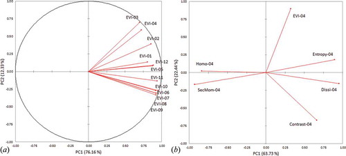
The first PCA was applied to EVI images and to texture indices, to select the most representative dates. The results achieved for the whole indices (e.g. EVI in Figure 2(a)) led to the selection of the months of January, April, and September, corresponding to the winter, spring, and autumn images. The second PCA was therefore applied to all indices (EVI and textural indices) corresponding to the three selected months (e.g. April in Figure 2(b)). The results of the second PCA indicate that entropy and dissimilarity are positively correlated, whereas they are negatively correlated to the second moment and homogeneity. Contrast is slightly correlated to any texture index. EVI is poorly correlated to any texture index. Therefore, because of a very poor correlation with EVI data, no textural index was eliminated for the study.

Figure 2. PCA results: (a) projection on the two first factors (PC1 and PC2) of the monthly average EVI images; (b) projection on the two first factors (PC1 and PC2) of the five texture indices (Dissi, Dissimilarity; SecMom, Second Moment; Homo, Homogeneity) and EVI for the month April (04).

Figure 3 presents the results obtained by calculating the Zang and Johnson indices, for different values of the scale parameter, from the unsupervised evaluation methods. The best results were identified as those obtained from the combination of EVI and second moment as its curve better corresponds to the optimal shape, with the Johnson and Zhang indices decreasing until a minimum and then increasing (Figure 3). The best scale parameter value is estimated to be between 15 and 20, for which the minimum values of both indices are identified. This analysis leads to the selection of input data and parameters that are similar to the previous study regarding the whole French territory (Bisquert, Bégué, and Deshayes 2015). The segmentation based on EVI, for three dates, second moment texture index, and a scale parameter fixed at 15, results in 56 HLUs.

Figure 3. Results (Johnson’s and Zhang’s curves) obtained using three dates of EVI and each of the five texture indices averaged over five years (2007–2011): (a) second moment, (b) contrast, (c) dissimilarity, (d) homogeneity, and (e) entropy.

3.1.2. Strata definition

Among the 56 strata obtained, 39 were identified as unprocessable strata. Among these 39, 27 were merged with their adjacent strata, and 12 strata remained without enough similarity with other adjacent strata to be merged. These 12 strata, with limited forest area, are covered mainly by agricultural land. They were set aside from this study. Finally, after merging and selecting the HLU, the study area was divided in 25 strata covering most of the forest area (Figure 4).

Figure 4. Stratification of the study area obtained after merging and eliminating unprocessable strata.

3.1.3. Stratum topographical and landscape indices

The 25 strata obtained are generally East–West oriented, such as the mountain range, but are of variable shape and dimensions, as shown in Figure 4. The value of the eight landscape indices were calculated for the 25 strata. Table 4 shows the minimum, maximum, mean, and standard deviation values for each index. Most of the values show great variability, to be related to the diversity of landscapes and forest cover of the area.

Table 4. Values calculated for the eight landscape indices describing the 25 strata.

Index	Min.	Max.	Mean	Standard deviation
Topographical indices
Area (ha)	13,242	917,244	240,950	212,307
Elevation (standard deviation) (m)	100	543	257	127
Slope (average) (°)	3	22	10	5
Area-derived and spatial organization landscape indices
Total forest-cover rate (%)	29	92	71	20
Patch area (average) (ha)	80	15,715	3054	3543
Patch area (standard deviation) (ha)	19	205	72	52
Composition landscape indices
Number of classes	3	23	11	6
Shannon Diversity index	1.35	2.77	2.07	0.41

3.2. Effect of stratification on classification accuracy

3.2.1. Global analysis

The supervised classifications were carried out for the whole area and for each stratum, for the two studied periods, using NDVI and EVI series. The use of stratification led to increased κ values from 0.53 and 0.52 to 0.65 and 0.64, for NDVI, and from 0.47 and 0.44 to 0.57 and 0.56, for EVI  (Table 5). Simultaneously, the use of stratification leads to an increase of the RF value from 6% to 13%. Stratification therefore not only leads to an increase of the number of well-classified pixels, but also leads to an increase of the proportion of unclassified pixels. There is no difference between the two studied periods. Using stratification, κ increased more than 0.1 for both vegetation indices, but NDVI gave systematically better results than EVI. From here, we chose to present only the results for NDVI and for the 2007–2009 period.

Table 5. Accuracy assessment obtained with and without stratification for the two studied periods (kappa coefficient (κ) and reject fraction).

Date	Classification	NDVI Global kappa coefficient (κ)	EVI Global kappa coefficient (κ)	Global reject fraction (RF) (%)
2007–2009	Without stratification	0.53	0.47	6
	With stratification	0.65	0.57	13
2009–2011	Without stratification	0.52	0.44	7
	With stratification	0.64	0.56	13

The PA values for each class, with and without stratification, and their differences are presented in Table 6. For each class, the PA values were improved using stratification. The values average increase from 51% to 66%. The values are also less scattered, with the PA standard deviation decreasing from 20% to 13%. The user’s accuracy values present similar results, the mean increasing from 47% to 62% and the standard deviation decreasing from 21% to 13%. This effect is not homogeneous for all classes. Wooded garrigue is the class with the minimum PA, rising from 13% without stratification to 40% with stratification. Monterrey pine is the class with the maximum PA, 93% and 96%, respectively, without and with stratification.

Table 6. Stratification effect on the producer’s accuracy, NDVI series for the 2007–2009 period.

	Producer’s accuracy (PA) (%)
Class	Without stratification	With stratification	Differences with – without	Group
Beech	74	75	1	1
Alpine heathland	63	64	1
Holm oak	58	59	1
Beech and silver fir	60	63	3
Monterey pine	93	96	3
Spanish matorral	54	60	6
Unwooded garrigue	70	80	10	2
Aleppo pine	61	70	10
Mountain pine	66	77	11
Scots pine	57	69	12
Pyrenean pine	52	64	12
Alpine grassland	54	69	15
Mixed deciduous forest	55	72	16
Grassland	57	74	17
Silver fir	61	79	18
Mixed mountain deciduous forest	20	46	26	3
Mountain Spanish matorral	24	50	26
Wooded garrigue	13	40	27
Mountain heathland	38	67	29
Pyrenean oak	40	69	29
Evergreen oaks	14	48	33
Deciduous oaks	30	64	34
Mean	51	66
St. dev.	20	13

Sorting out the UA difference values with and without stratification, three groups of classes could be distinguished (Table 6). The first group is the one for which the stratification effect is poor (from 1% to 6%). These classes were initially well classified (PA values higher than 54%), mostly mono-specific forest types (beech, Monterrey pine). However, mixed natural vegetation types (shrubland, heathland) or forest classes (mixed beech and silver fir) were found in this group too. The second group presents good PA values (from 52% to 70%) and an average increase (+13%). In this group, we found pine forest classes and some non-woody ones (grassland, garrigue).

Finally, the classes with the smallest initial values (lower than 40%) are the most improved by the use of stratification (+29% on average). With stratification, all user’s accuracy values become greater than 40%. This group is mainly formed by heterogeneous classes, mixed species (deciduous and evergreen oaks, mixed deciduous), or non-woody mixed types (garrigue, shrubland, heathland). Analysis of the error matrices showed that most errors were observed between mono-species forest types and the mixed forest types, partially composed of the same species. The phenomenon is, for instance, observed for silver fir and mixed beech-silver fir forest.

The thematic distribution of the RF between the different classes is the rate between the number of rejected pixels corresponding to one class and the total RF. It appears similar to the relative area of each class of the forest map. As previously noted, the thematic quality gain is combined to an increase of 6–7% of the RF. However, there is no significant distribution change; this increase is homogeneous for all classes.

3.2.2. Per-stratum analysis

Stratification globally improves κ but also increases RF. This effect is also true for each stratum considered individually, but is extremely variable from one stratum to another. Figure 5 shows that without using stratification, a few strata present small κ values (lower than 0.3 for five strata) and most of them present κ values around 0.5. Most strata (20) have κ values ranging between 0.3 and 0.7. RF is around the mean (6%), and only two strata have an RF value greater than 10%. The use of stratification improves the κ values of all the strata. Most of the strata (23 out of 25) have a κ value greater than 0.5. However, an increase of the RF, nearly proportional to that of κ, is noted. The RF values are all greater than 10%. Despite the overall value of 13%, eight strata present an RF value greater than 20%.

Figure 5. κ and RF values for the 25 strata with and without stratification.

From the previous results, it is noted that the strata that present the most important κ gains also present the most important RF rise. In Figure 6, the relationship between κ difference and RF difference indicates a highly significant and positive correlation between those two indicators.

Figure 6. Relation between κ and RF differences with and without stratification for the 25 strata.

The relationship between the distribution of the κ values (with and without stratification) and the stratum area enables one to identify three sets of strata, depending on their area (Figure 7): small-area strata, lower than 200,000 ha; an intermediate set, of area ranging between 200,0000 ha and 450,0000 ha; and a very-large-area strata, greater than 450,000 ha. This strata characterization, according to their area, will be repeated on the following figures and will be used as a baseline for the following interpretation of results.

Figure 7. (a) Relation between the per-stratum kappa coefficient (κ) value with stratification and the stratum area (ha). (b) Relation between the per-stratum κ value without stratification and the stratum area (ha).

3.3. Influence of the topographical and landscape indices

Coefficient of determination (R²) between the topographical and landscape indices and the κ and RF differences enabled one to identify the influence of these indices on stratification efficiency (Table 7). It should be recalled that the differences between κ and RF linked to stratification systematically increased. Significant relations (R² values greater than 0.25) were observed between the κ and RF differences and the landscape indices. For the topographical indices, the relationships are negative; they are significant at the 0.01 level, except between the mean slope and the RF difference. Among the area-derived indices, only the patch area standard deviation has a significant positive correlation with the κ and RF differences. The class number has a significant negative correlation, but not the Diversity Shannon index.

Table 7. Coefficient of determination (R²) between the stratum indicators and the per-stratum κ and RF differences for the 2007–2009 period (bold: significant for α = 0.01; (+): positive correlation; (-): negative correlation).

Index	κ difference	RF difference
Topographical indices
Stratum area (ha)	(-) 0.32	(-) 0.35
Elevation (standard deviation) (m)	(-) 0.38	(-) 0.31
Slope (mean) (°)	(-) 0.28	(-) 0.18
Area-derived landscape indices
Total forest-cover rate	(-) 0.09	(-) 0.11
Patch area (average) (ha)	(+) 0.07	(+) 0.003
Patch area (standard deviation) (ha)	(+) 0.64	(+) 0.59
Composition landscape indices
Number of classes	(-) 0.34	(-) 0.42
Diversity Shannon index	(-) 0.10	(-) 0.15

3.3.1. Influence of stratum area

A significant negative correlation was observed for the κ and RF differences (Table 6). The graphical representation of the relation between the stratum area and the κ and RF differences (Figure 8) and the study of the classified vegetation area (Figure 9) enable one to differentiate the strata into three distinct groups.

Figure 8. Relation between stratum area (ha) and κ difference.

Figure 9. Classified vegetation area (ha) – strata order by group and increasing with stratum area.

Group A, with four strata, each with an area greater than 450,000 ha, presents low classification accuracy improvements (κ difference lower than 0.1) and a poor RF increase (4–5% difference). As shown in Figure 9, group A strata are characterized by a classified vegetation area greater than 120,000 ha. Group C, with three strata, each with a very small area (lower than 100,000 ha), presents a very high κ difference and a very small κ value without stratification (between 0.06 and 0.36). The κ gain does not reflect an improvement of classification accuracy as it is linked to a very high RF, varying from 20% to 40%. Other strata have an area lower than 100,000 ha; however, their RF does not exceed 22% and their κ value without stratification is around 0.5. Group C strata are characterized by a classified vegetation area lower than 5000 ha (Figure 9), which can be considered as a critical threshold. Finally, group B contains most of the strata (18), their areas being very variable, but lower than 450,000 ha. In this group, the κ and RF differences are also very variable. In these situations, the relation between the κ difference and the strata area is not significant (Figure 8).

Although the relation between the stratum area and κ gain is linear and negative if the whole strata are considered, the three distinct groups A, B, and C must be independently considered for the interpretation of the results. This leads to the conclusion that if both extreme situations (groups A and C) are not considered, the improvement of classification is not related to the stratum area.

3.3.2. Influence of elevation standard deviation

For the whole 25 strata, the relations between the elevation standard deviation and the κ and RF differences are significant, with respective R² values of 0.38 and 0.31 (Table 7). However, for group B, the relation is not significant, with an R² value of 0.16 for the κ difference and of 0.09 for the RF difference. Thus, the elevation factor, and more precisely, the mountainous and uneven strata characteristics with the absence of relation of slopes, is not an influential factor of stratification efficiency. No threshold effect can hence be identified (Figure 10). For group A, an indirect effect of area on the results can be assumed, the biggest strata presenting the largest elevation standard deviation. Group C keeps its atypical characteristics; these strata are situated in the piedmont, in less uneven zones.

3.3.3. Influence of the standard deviation of the patches area

For the whole 25 strata, the correlation between this indicator and the κ and RF differences (with the respective R² values of 0.64 and 0.59) is significant and positive. The standard deviation of the patches area is the indicator presenting the highest R² values (Table 7). However, if the single group B is considered, the correlation is not significant for the κ difference, which cannot show a direct influence between the standard deviation of the patches area and the classification accuracy (Figure 11). The correlation remains significant for the RF difference. As the standard deviation of the patches area can be considered as a fragmentation indicator, the hypothesis could be that the higher its value, the more emphasized the fragmentation, which increases the RF by enhancing the border effect. Groups A and B are still separate on the graph, which attests the indirect influence of the stratum area.

Figure 10. Relation between the standard deviation of elevation (m) and the κ difference considering the strata groups A, B, and C.

Figure 11. Relation between standard deviation of the patch area (ha) and κ difference considering the strata groups A, B, and C.

3.3.4. Influence of the number of classes

As in the above-mentioned cases, the relation between the number of classes and the κ and RF differences is significant and negative for most of the 25 strata, with the respective R² values of 0.34 and 0.42 (Table 7). However, when only group B is taken into account, the small R² values (0.008 for the κ difference and 0.13 for the RF difference) indicate an absence of significant relation with this index. The Shannon index, which also characterizes the composition of the forest cover of the strata, is not significantly correlated to the κ and RF differences. This must be linked to the calculation of this index, partly based in the stratum area (Figure 12).

Figure 12. Relation between number of classes and κ difference considering the strata groups A, B, and C.

No other indices (total forest-cover rate, mean slope, average patches area, diversity Shannon index) present significant correlations with the κ and RF differences (Table 7). Topography, composition, and fragmentation of forest types therefore seem to have no influence on stratification efficiency.

4. Discussion

The results of this study showed that the use of stratification performed from a coarse spatial resolution time series and from an OBIA process significantly improves the supervised classification accuracy for our study area. This improvement is similar for the two studied periods (2007–2009 and 2009–2011) with, in both cases, a κ value calculated at a global scale increasing by 0.12. However, this improvement is accompanied by an increase of the RF of 6–7% at a global scale, for both periods. These global increases also occur when the results are analysed per stratum: the κ and RF rise. The spread of κ values is lower when stratification is used. A total of 22 forest and natural vegetation-type classes have been distinguished, with a varying accuracy level without stratification increasing from 13% to 93%. The use of stratification improves the user’s accuracy for all classes; finally, it varies from 40% to 80%. The improvement is more important for the types presenting an initial low accuracy value.

The characteristics of the strata have an influence on classification accuracy, and the most influential is stratum area. Two essential elements were demonstrated: first, the relation between stratum area and classification accuracy is significant. Second, minimum and maximum thresholds were identified for the stratum area, and therefore the vegetation classified area. If the strata area is over 450,000 ha and the vegetation classified area is greater than 120,000 ha, then the κ value improvements are extremely poor. If the strata area is smaller than 100,000 ha and the vegetation classified area is lower than 5000 ha, the results are notably degraded because of the very high RF. These thresholds can be integrated as recommendations for the stratification process. During the OBIA segmentation process, the stratum area is related to the scale parameter value, whose setting is important. Fixing this parameter value to 15, before the merging step, we defined 30 HLU with an area lower than 100,000 ha and one higher than 450,000 ha (Table 8). Choosing 20 as the scale parameter value resulted in 39 HLU, 15 with area lower than 100,000 ha and two higher than 450,000 ha. The number of unprocessable strata is, respectively, 39 and 31.

Table 8. Segmentation results according to 15 and 20 scale parameter values.

Scale parameter		15	20
number of HLU:	total	56	39
number of HLU:	area < 100,000 ha	30	15
number of HLU:	100,000 < area < 450,000 ha	25	22
number of HLU:	area > 450,000 ha	1	2
number of unprocessed strata		39	31

The optimum value for scale parameter is 15 or 20; indeed, for values lower than 15 or greater than 20, the number of unprocessable strata would rise, either for small- or large-area strata. The choice of the two main parameters of the OBIA processing, that is, fixing the scale parameter at 15 and selecting the second moment as the texture index, is identical to the original study at the scale of the French territory (Bisquert, Bégué, and Deshayes 2015). This confirms the robustness and reproducibility of this stratification method. Similar works were carried out in Mali (Vintrou et al. 2012) and led to different choices for the texture index. These differences can be linked to different landscape characteristics. This method, originally developed for landscape mapping, can now be recommended to improve forest-cover mapping in regions with high topographical and climatic variability. When used for classification, a merging step of the smallest strata is necessary. It can easily be carried out with the statistical approach suggested in this study, taking into account the similarity of land cover. The subdivision of the too large strata can easily be carried out using photointerpretation.

5. Conclusion

The landscape analysis stratification approach has the same efficiency level as the usual approaches encountered in the literature (Bauer et al. 1994). Only easily accessible remote-sensing data have been used and this method does not have to rely on existent thematic map or on expert knowledge. The analysis of the strata landscape characteristics leads to strata definition operational items that could be used to adjust the parameters while creating HLU and defining the strata. These items are usually area thresholds (total area and area to classify). The analysis of quality indicators shows that only κ is not sufficient to appreciate the results; it has to be balanced by an RF analysis. The obtained results enable one to conclude that the use of object segmentation as a stratification tool, in the case of a probabilistic approach, applied by pixel, improves those classification results. Despite the use of a detailed forest nomenclature (about 20 classes), the quality obtained is satisfying. This stratification tool therefore enables one to gain global accuracy besides increasing the user’s accuracy for each class. The study did not identify a particular influence of topographical and landscape stratum characteristics on stratification. It however brought to light a maximum threshold effect of the stratum area, beyond which no improvement was observed (about 450,000 ha for this study). Below a certain minimum stratum area value (100,000 ha for our study), critical conditions might occur for supervised classification, corresponding to an undersized training data set. We can thus conclude that the implementation of such a stratification must depend on a preliminary checkout of the OBIA parameters.

These first results, however, show that the applied OBIA method could be an objective and reproducible alternative to expert knowledge stratification. The question of the reproducibility of this method at a finer spatial resolution arises with the perspective of the arrival of future Sentinel-2 data. They will enable one to combine high temporal and high spatial resolution, which will be a definite contribution to the vegetation classification of large-area territories. The notion of vegetation landscape texture as well as spatial definition of forest types and their signatures from the vegetation index will be approached at another scale. It will be the same for object segmentation. In this context, the perspective of enhancing this study would consist in studying the action of stratification on such a time series.

Disclosure statement

No potential conflict of interest was reported by the authors.

References

- Alcaraz-Segura, D., J. Paruelo, and J. Cabello. 2006. “Identification of Current Ecosystem Functional Types in the Iberian Peninsula.” Global Ecology and Biogeography 15 (2): 200–212. doi:10.1111/geb.2006.15.issue-2.
- Balthazar, V., V. Vanacker, and E. F. Lambin. 2012. “Evaluation and Parameterization of ATCOR3 Topographic Correction Method for Forest Cover Mapping in Mountain Areas.” International Journal of Applied Earth Observation and Geoinformation 18 (0): 436–450. doi:10.1016/j.jag.2012.03.010.
- Bauer, M. E., T. E. Burk, A. R. Ek, P. R. Coppin, S. D. Lime, T. A. Walsh, D. K. Walters, and W. Befort. 1994. “Satellite Inventory of Minnesota Forest Resources.” Photogrammetric Engineering and Remote Sensing 60 (3): 287–298.
- Bisquert, M., A. Bégué, and M. Deshayes. 2015. “Object-Based Delineation of Homogeneous Landscape Units at Regional Scale Based on MODIS Time Series.” International Journal of Applied Earth Observation and Geoinformation 37: 72–82. doi:10.1016/j.jag.2014.10.004.
- Blaschke, T. 2010. “Object Based Image Analysis for Remote Sensing.” ISPRS Journal of Photogrammetry and Remote Sensing 65 (1): 2–16. doi:10.1016/j.isprsjprs.2009.06.004.
- Blaschke, T., G. J. Hay, M. Kelly, S. Lang, P. Hofmann, E. Addink, R. Queiroz Feitosa, et al. 2014. “Geographic Object-Based Image Analysis - Towards a New Paradigm.” ISPRS Journal of Photogrammetry and Remote Sensing 87 (0): 180–191. doi:10.1016/j.isprsjprs.2013.09.014.
- Blesius, L., and F. Weirich. 2005. “The Use of the Minnaert Correction for Land‐Cover Classification in Mountainous Terrain.” International Journal of Remote Sensing 26 (17): 3831–3851. doi:10.1080/01431160500104194.
- Boyd, D. S., and F. M. Danson. 2005. “Satellite Remote Sensing of Forest Resources: Three Decades of Research Development.” Progress in Physical Geography 29 (1): 1–26. doi:10.1191/0309133305pp432ra.
- Broich, M., S. V. Stehman, M. C. Hansen, P. Potapov, and Y. E. Shimabukuro. 2009. “A Comparison of Sampling Designs for Estimating Deforestation from Landsat Imagery: A Case Study of the Brazilian Legal Amazon.” Remote Sensing of Environment 113 (11): 2448–2454. doi:10.1016/j.rse.2009.07.011.
- Cai, H., S. Zhang, K. Bu, J. Yang, and L. Chang. 2011. “Integrating Geographical Data and Phenological Characteristics Derived from MODIS Data for Improving Land Cover Mapping.” Journal of Geographical Sciences 21 (4): 705–718. doi:10.1007/s11442-011-0874-1.
- Carrão, H., P. Gonçalves, and M. Caetano. 2007. “Use of Intra-Annual Satellite Imagery Time-Series for Land Cover Characterization Purpose.” Paper presented at the Proceedings of the 26th EARSeL Symposium, May 29-June 2, Warsaw, Poland.
- Carrão, H., P. Gonçalves, and M. Caetano. 2008. “Contribution of Multispectral and Multitemporal Information from MODIS Images to Land Cover Classification.” Remote Sensing of Environment 112 (3): 986–997. doi:10.1016/j.rse.2007.07.002.
- Cihlar, J. 2000. “Land Cover Mapping of Large Areas from Satellites: Status and Research Priorities.” International Journal of Remote Sensing 21 (6–7): 1093–1114. doi:10.1080/014311600210092.
- Clark, M. L., T. M. Aide, H. R. Grau, and G. Riner. 2010. “A Scalable Approach to Mapping Annual Land Cover at 250 M Using MODIS Time Series Data: A Case Study in the Dry Chaco Ecoregion of South America.” Remote Sensing of Environment 114 (11): 2816–2832. doi:10.1016/j.rse.2010.07.001.
- Colditz, R. R., M. Schmidt, C. Conrad, M. C. Hansen, and S. Dech. 2011. “Land Cover Classification with Coarse Spatial Resolution Data to Derive Continuous and Discrete Maps for Complex Regions.” Remote Sensing of Environment 115 (12): 3264–3275. doi:10.1016/j.rse.2011.07.010.
- Congalton, R. G. 1991. “A Review of Assessing the Accuracy of Classifications of Remotely Sensed Data.” Remote Sensing of Environment 37: 35–46. doi:10.1016/0034-4257(91)90048-B.
- Daubet, B., S. De Miguel Magaña, and A. Maurette. 2007. Livre Blanc des forêts Pyrénéennes, pour une gestion durable des Pyrénées. GEIE FORESPIR 78.
- DeFries, R., M. Hansen, and J. Townshend. 1995. “Global Discrimination of Land Cover Types from Metrics Derived from AVHRR Pathfinder Data.” Remote Sensing of Environment 54 (3): 209–222. doi:10.1016/0034-4257(95)00142-5.
- Delincé, J. 2001. “A European Approach to Area Frame Surveys.” Paper presented at the Conference on Agricultural and Environmental Statistical Applications (CAESAR), Rome, June 5–7.
- Dymond, C. C., D. J. Mladenoff, and V. C. Radeloff. 2002. “Phenological Differences in Tasseled Cap Indices Improve Deciduous Forest Classification.” Remote Sensing of Environment 80 (3): 460–472. doi:10.1016/S0034-4257(01)00324-8.
- Evans, J. P., and R. Geerken. 2006. “Classifying Rangeland Vegetation Type and Coverage Using a Fourier Component Based Similarity Measure.” Remote Sensing of Environment 105 (1): 1–8. doi:10.1016/j.rse.2006.05.017.
- Foody, G. M. 2002. “Status of Land Cover Classification Accuracy Assessment.” Remote Sensing of Environment 80 (1): 185–201. doi:10.1016/S0034-4257(01)00295-4.
- Foody, G. M., R. M. Lucas, P. J. Curran, and M. Honzak. 1997. “Mapping Tropical Forest Fractional Cover from Coarse Spatial Resolution Remote Sensing Imagery.” Plant Ecology 131 (2): 143–154. doi:10.1023/A:1009775619936.
- Forman, R. T. T., and M. Godron. 1981. “Patches and Structural Components for A Landscape Ecology.” Bioscience 31 (10): 733–740. doi:10.2307/1308780.
- Forman, R. T. T., and R. Godron. 1986. Landscape Ecology. Chichester, New York: Wiley.
- Friedl, M. A., D. K. McIver, J. C. F. Hodges, X. Y. Zhang, D. Muchoney, A. H. Strahler, C. E. Woodcock, et al. 2002. “Global Land Cover Mapping from MODIS: Algorithms and Early Results.” Remote Sensing of Environment 83 (1–2): 287–302. doi:10.1016/S0034-4257(02)00078-0.
- Friedl, M. A., D. Sulla-Menashe, B. Tan, A. Schneider, N. Ramankutty, A. Sibley, and X. Huang. 2010. “MODIS Collection 5 Global Land Cover: Algorithm Refinements and Characterization of New Datasets.” Remote Sensing of Environment 114 (1): 168–182. doi:10.1016/j.rse.2009.08.016.
- Gallego, F. J., and H. J. Stibig. 2013. “Area Estimation from a Sample of Satellite Images: The Impact of Stratification on the Clustering Efficiency.” International Journal of Applied Earth Observation and Geoinformation 22 (0): 139–146. doi:10.1016/j.jag.2012.03.003.
- Ganguly, S., M. A. Friedl, B. Tan, X. Zhang, and M. Verma. 2010. “Land Surface Phenology from MODIS: Characterization of the Collection 5 Global Land Cover Dynamics Product.” Remote Sensing of Environment 114 (8): 1805–1816. doi:10.1016/j.rse.2010.04.005.
- García-Mora, T. J., J.-F. Mas, and E. A. Hinkley. 2012. “Land Cover Mapping Applications with MODIS: A Literature Review.” International Journal of Digital Earth 5 (1): 63–87. doi:10.1080/17538947.2011.565080.
- Gertner, G., G. Wang, A. B. Anderson, and H. Howard. 2007. “Combining Stratification and Up-Scaling Method-Block Cokriging with Remote Sensing Imagery for Sampling and Mapping an Erosion Cover Factor.” Ecological Informatics 2 (4): 373–386. doi:10.1016/j.ecoinf.2007.06.002.
- Giri, C., B. Pengra, J. Long, and T. R. Loveland. 2013. “Next Generation of Global Land Cover Characterization, Mapping, and Monitoring.” International Journal of Applied Earth Observation and Geoinformation 25 (0): 30–37. doi:10.1016/j.jag.2013.03.005.
- Hay, G. J., and G. Castilla. 2006. “Object-Based Image Analysis: Strengths, Weaknesses, Opportunities and Threats (SWOT).” Paper presented at the 1st International Conference on Object-based Image Analysis (OBIA 2006) Salzburg University, Austria.
- Homer, C., and A. Galant. 2001. “Partitioning the Conterminous United States into Mapping Zones for Landsat TM Land Cover Mapping.” In USGS Draft White Paper. USGS Survey report.
- Homer, C., C. Q. Huang, L. M. Yang, B. Wylie, and M. Coan. 2004. “Development of a 2001 National Land-Cover Database for the United States.” Photogrammetric Engineering & Remote Sensing 70 (7): 829–840. doi:10.14358/PERS.70.7.829.
- Homer, C., R. Ramsey, T. Edwards, and A. Falconer. 1997. “Landscape Cover-Type Modeling Using a Multi-Scene Thematic Mapper Mosaic.” Photogrammetric Engineering & Remote Sensing 63 (1): 59–67.
- Huete, A., K. Didan, T. Miura, E. P. Rodriguez, X. Gao, and L. G. Ferreira. 2002. “Overview of the Radiometric and Biophysical Performance of the MODIS Vegetation Indices.” Remote Sensing of Environment 83 (1–2): 195–213. doi:10.1016/S0034-4257(02)00096-2.
- Hüttich, C., U. Gessner, M. Herold, B. Strohbach, M. Schmidt, M. Keil, and S. Dech. 2009. “On the Suitability of MODIS Time Series Metrics to Map Vegetation Types in Dry Savanna Ecosystems: A Case Study in the Kalahari of NE Namibia.” Remote Sensing 1 (4): 620–643. doi:10.3390/rs1040620.
- Jarvis, A., H. I Reuter, A. Nelson, and E. Guevara. 2008. Hole-filled SRTM for the globe Version 4. CGIAR-CSI SRTM 90m Database. Available from http://srtm.csi.cgiar.org.
- Johnson, B., and Z. Xie. 2011. “Unsupervised Image Segmentation Evaluation and Refinement Using a Multi-Scale Approach.” ISPRS Journal of Photogrammetry and Remote Sensing 66 (4): 473–483. doi:10.1016/j.isprsjprs.2011.02.006.
- Jönsson, P., and L. Eklundh. 2004. “TIMESAT—A Program for Analyzing Time-Series of Satellite Sensor Data.” Computers 30 (8): 833–845. doi:10.1016/j.cageo.2004.05.006.
- Justice, C. O., B. N. Holben, and M. D. Gwynne. 1986. “Monitoring East African Vegetation Using AVHRR Data.” International Journal of Remote Sensing 7 (11): 1453–1474. doi:10.1080/01431168608948948.
- Krishna Prasad, V., K. V. S. Badarinath, and A. Eaturu. 2007. “Spatial Patterns of Vegetation Phenology Metrics and Related Climatic Controls of Eight Contrasting Forest Types in India - Analysis from Remote Sensing Datasets.” Theoretical and Applied Climatology 89 (1–2): 95–107. doi:10.1007/s00704-006-0255-3.
- Kuemmerle, T., V. C. Radeloff, K. Perzanowski, and P. Hostert. 2006. “Cross-Border Comparison of Land Cover and Landscape Pattern in Eastern Europe Using a Hybrid Classification Technique.” Remote Sensing of Environment 103 (4): 449–464. doi:10.1016/j.rse.2006.04.015.
- Lê, S., J. Josse, and F. Husson. 2008. “Factominer: An R Package for Multivariate Analysis.” Journal of Statistical Software 25 (1): 1–18. doi:10.18637/jss.v025.i01.
- Lillesand, T. M. 1996. “A Protocol for Satellite-Based Land Cover Classification in the Upper Midwest.” In Gap Analysis: A Landscape Approach to Biodiversity Planning, edited by J. Scott, T. Tear, and F. Davis, 320, ASPRS.
- Nagendra, H. 2001. “Using Remote Sensing to Assess Biodiversity.” International Journal of Remote Sensing 22 (12): 2377–2400. doi:10.1080/01431160117096.
- Otukei, J. R., and T. Blaschke. 2010. “Land Cover Change Assessment Using Decision Trees, Support Vector Machines and Maximum Likelihood Classification Algorithms.” International Journal of Applied Earth Observation and Geoinformation 12 (0): S27–S31. doi:10.1016/j.jag.2009.11.002.
- Pettinger, L. R. 1982. “Digital Classification of Landsat Data for Vegetation and Land-Cover Mapping in the Blackfoot River Watershed, Southeastern Idaho.” In U. S. Geological Survey Professional Paper, edited by USGS.
- Pettorelli, N., J. O. Vik, A. Mysterud, J.-M. Gaillard, C. J. Tucker, and N. C. Stenseth. 2005. “Using the Satellite-Derived NDVI to Assess Ecological Responses to Environmental Change.” Trends in Ecology & Evolution 20 (9): 503–510. doi:10.1016/j.tree.2005.05.011.
- Redo, D. J., and A. C. Millington. 2011. “A Hybrid Approach to Mapping Land-Use Modification and Land-Cover Transition from MODIS Time-Series Data: A Case Study from the Bolivian Seasonal Tropics.” Remote Sensing of Environment 115 (2): 353–372. doi:10.1016/j.rse.2010.09.007.
- Reese, H. M., T. M. Lillesand, D. E. Nagel, J. S. Stewart, R. A. Goldmann, T. E. Simmons, J. W. Chipman, and P. A. Tessar. 2002. “Statewide Land Cover Derived from Multiseasonal Landsat TM Data: A Retrospective of the WISCLAND Project.” Remote Sensing of Environment 82 (2–3): 224–237. doi:10.1016/S0034-4257(02)00039-1.
- Ren, G., A.-X. Zhu, W. Wang, W. Xiao, Y. Huang, G. Li, D. Li, and J. Zhu. 2009. “A Hierarchical Approach Coupled with Coarse DEM Information for Improving the Efficiency and Accuracy of Forest Mapping over Very Rugged Terrains.” Forest Ecology and Management 258 (1): 26–34. doi:10.1016/j.foreco.2009.03.043.
- Rouse, J. W., R. H. Haas, J. A. Schell, and D. W. Deering. 1973. “Monitoring Vegetation Systems in the Great Plains with ERTS.” Paper presented at the Third ERTS Symposium, Washington, DC.
- Shannon, C. E. 1948. “A Mathematical Theory of Communication.” Bell System Technical Journal 27 (3): 379–423. doi:10.1002/j.1538-7305.1948.tb01338.x.
- Soubeyroux, J. M., S. Jourdain, D. Grimal, F. Espejo Gil, P. Esteban, and T. Merz. 2011. “Global Approach for Inventory and Applications of Climate Data on the Pyrenees Chain.” In Colloque SHF: “Eaux en montagne”, Lyon, France, 7.
- Spearman, C. 1904. ““General Intelligence,” Objectively Determined and Measured.” The American Journal of Psychology 15 (2): 201–292. doi:10.2307/1412107.
- Stehman, S. V. 2009. “Sampling Designs for Accuracy Assessment of Land Cover.” International Journal of Remote Sensing 30 (20): 5243–5272. doi:10.1080/01431160903131000.
- Stehman, S. V., and R. L. Czaplewski. 1998. “Design and Analysis for Thematic Map Accuracy Assessment: Fundamental Principles.” Remote Sensing of Environment 64 (3): 331–344. doi:10.1016/S0034-4257(98)00010-8.
- Stehman, S. V., M. C. Hansen, M. Broich, and P. V. Potapov. 2011. “Adapting a Global Stratified Random Sample for Regional Estimation of Forest Cover Change Derived from Satellite Imagery.” Remote Sensing of Environment 115 (2): 650–658. doi:10.1016/j.rse.2010.10.009.
- Sulla-Menashe, D., M. A. Friedl, O. N. Krankina, A. Baccini, C. E. Woodcock, A. Sibley, G. Sun, V. Kharuk, and V. Elsakov. 2011. “Hierarchical Mapping of Northern Eurasian Land Cover Using MODIS Data.” Remote Sensing of Environment 115 (2): 392–403. doi:10.1016/j.rse.2010.09.010.
- Tsaneva, M. G., D. D. Krezhova, and T. K. Yanev. 2010. “Development and Testing of a Statistical Texture Model for Land Cover Classification of the Black Sea Region with MODIS Imagery.” Advances in Space Research 46 (7): 872–878. doi:10.1016/j.asr.2010.05.011.
- Tucker, C. J., and P. J. Sellers. 1986. “Satellite Remote Sensing of Primary Production.” International Journal of Remote Sensing 7 (11): 1395–1416. doi:10.1080/01431168608948944.
- Turner, M. G. 1989. “Landscape Ecology: The Effect of Pattern on Process.” Annual Review of Ecology and Systematics 20 (1): 171–197. doi:10.1146/annurev.es.20.110189.001131.
- Vintrou, E., A. Desbrosse, A. Bégué, S. Traoré, C. Baron, and D. Lo Seen. 2012. “Crop Area Mapping in West Africa Using Landscape Stratification of MODIS Time Series and Comparison with Existing Global Land Products.” International Journal of Applied Earth Observation and Geoinformation 14 (1): 83–93. doi:10.1016/j.jag.2011.06.010.
- Xie, Y., Z. Sha, and M. Yu. 2008. “Remote Sensing Imagery in Vegetation Mapping: A Review.” Journal of Plant Ecology 1 (1): 9–23. doi:10.1093/jpe/rtm005.
- Zhang, X., P. Xiao, and X. Feng. 2012. “An Unsupervised Evaluation Method for Remotely Sensed Imagery Segmentation.” IEEE Geoscience and Remote Sensing Letters 9 (2): 156–160. doi:10.1109/lgrs.2011.2163056.
- Zhou, L., R. K. Kaufmann, Y. Tian, R. B. Myneni, and C. J. Tucker. 2003. “Relation between Interannual Variations in Satellite Measures of Northern Forest Greenness and Climate between 1982 and 1999.” Journal of Geophysical Research: Atmospheres 108 (D1): 4004. doi:10.1029/2002jd002510.