Combination of stereo SAR and InSAR for DEM generation using TanDEM-X spotlight data

ABSTRACT

The objective of this work is to generate accurate digital elevation models (DEMs) from synthetic aperture radar (SAR) interferograms using the spotlight and staring spotlight modes during the TanDEM-X (TDX) science phase. We use stereo SAR with TDX or TerraSAR-X (TSX) to estimate absolute heights of natural or man-made reflectors for input to the unwrapped interferograms. The accuracy of the absolute heights in the DEMs was a few decimetres in flat regions and a few metres in the hilly and rugged terrain.

1. Introduction

The twin satellites TerraSAR-X (TSX) and TanDEM-X (TDX) have been flying in formation for several years. TSX was launched on 15 June 2007 and TDX on 21 June 2010. An early detailed overview of the TDX mission can be found in Krieger et al. (2007). A more recent overview, including the secondary mission objectives, can be found in Krieger et al. (2013). The main purpose of the TDX mission is to generate a global digital elevation model (DEM) collecting bi-static SAR data almost simultaneously, which makes it possible to generate interferograms with high coherence. To improve the quality of the raw DEM, Gonzalez et al. (2010a; 2010b) proposed using accurate height references provided by the Ice, Cloud and land Elevation Satellite (ICESat) for calibration. Avtar et al. (2015) evaluated DEM generation using TDX data in Tokyo compared with several types of DEM data: lidar, local DEM, Advanced Spaceborne Thermal Emission and Reflection Radiometer (ASTER), and Shuttle Radar Topography Mission (SRTM). An analysis of the relative height errors for different ground characteristics was performed by Rizzoli et al. (2012). The most recent results on Global TDX DEM accuracy and high-resolution DEMs can be found in Wecklich et al. (2016), Wessel et al. (2016), Lachaise and Fritz (2016), and Gruber et al. (2016).

Eldhuset and Weydahl (2011) demonstrated that stereoSAR with TerraSAR alone using only seven data sets could yield absolute height accuracy of a few decimetres for the deployed corner reflectors (CRs). Gisinger et al. (2015) developed another technique for stereo height estimation where they avoided the two-step procedure described in Eldhuset and Weydahl (2011). They carried out a much more extensive study of position and height accuracy using three test sites and 130 data takes. Eldhuset and Weydahl (2011) found a residual Doppler (equivalent to the azimuth offset), which was of the same order as the azimuth residual found in Gisinger et al. (2015) in Figure 8 b for the TMSP v4.4 processor. The updated TMSP v4.5 and v4.6 were found to be more accurate.

Figure 1. Upper left image: TSX image of 9 March 2015 in Table 1 with the selected GCPs (G1–G7). The other images are zoomed around each of the encircled GCPs.

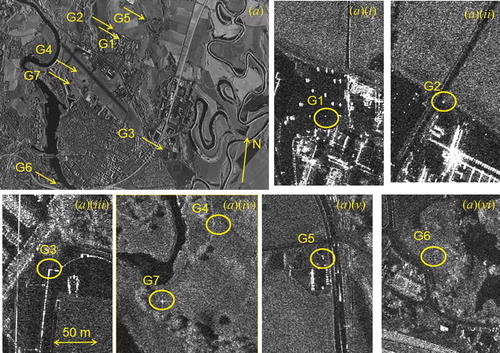
Figure 2. UTM geocoded staring spotlight image, 10 March 2015 in Table 1. Pixel spacing is 1.8 m for the Northing (vertical) and Easting (horizontal). Scene centre: 59 º 59ʹ 10ʺ N, 11º 3ʹ 0ʺ E.

Figure 3. UTM geocoded StInSAR-derived DEM, 10 March 2015 in Table 1. Pixel spacing is 1.8 m for the Northing and Easting.

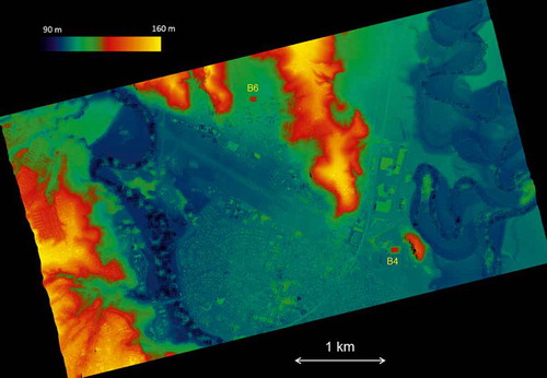
Figure 4. Sub-images of Figures 2 and 3 showing some buildings (B1–B5). B4 is shown in Figure 3.

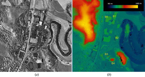
Figure 5. Staring spotlight image over Nikel in Russia on 4 February 2015 in Table 2. G1 is the GCP and A1–A3 are small regions for the estimation of height.

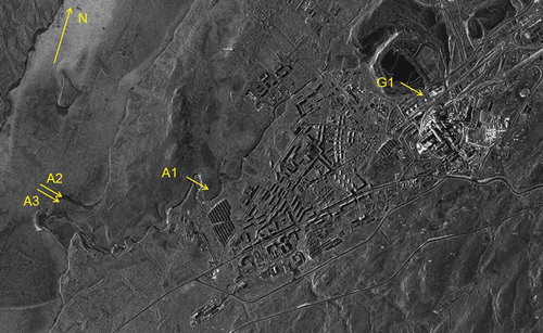
Figure 6. Interferogram from the same time and area as in Figure 5.

Figure 7. UTM geocoded DEM with a pixel spacing of 1.8 m derived from the interferogram in Figure 6. Scene centre: 69 º 24ʹ 36ʺ N, 30º 12ʹ 11ʺ E.

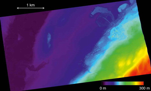
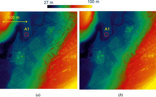
Figure 8. (a) UTM geocoded DEM of 22 December at incidence angle 47º in an area around the A1 point shown in Figure 5. (b) Average of six DEMs at 47º.

Eldhuset and Weydahl (2013) introduced a technique, called Stereo Interferometric SAR (StInSAR), where stereoSAR is used for estimation of the absolute height of ground control points (GCPs), which are used for the height estimation of interferograms. Only one interferogram was tested. We developed this software further for DEM generation using TDX scientific phase data Hajnsek et al. (2014). In this article, we use staring spotlight and high-resolution spotlight CoSSC (Co-registered Single-look Slant range Complex) data (Balss et al. 2014) from three test sites for evaluation of the absolute height accuracy in StInSAR-generated DEMs. The calibration strategy for generation of the Global TDX DEM uses ICEsat data as GCPs. The ICEsat data are historical data and changes might occur. The data set received in this work is used to validate the StInSAR software and show how very accurate absolute heights can be estimated without other data than TDX spotlight data.

2. TDX modes and data set

2.1 TDX modes

We received TDX CoSSC data during the science phase from German Aerospace Center (DLR) under an Announcement of Opportunity project (AO-project NTI_INS6664). The science phase started in October 2014 and was completed in December 2015. Within this time, two main interferometric operation modes were executed: the pursuit mono-static mode (October 2014–February 2015) and the bi-static mode (March 2015–December 2015). In the pursuit mono-static mode, the two satellites operated independently with an along-track distance of 76 km (10 s temporal separation). In the bi-static mode, the along-track distance was mostly less than 500 m and either TSX or TDX was used as a transmitter and both satellites received the scattered echo. For further details on the modes and science phase timeline, please refer to Hajnsek et al. (2014) and Tridon et al. (2014). The processing of CoSSC products has been described in Balss et al. (2014) and further information on SAR processing methods of staring spotlight data can be found in Mittermayer et al. (2014), Prats-Iraola et al. (2014), and Kraus et al. (2016).

2.2 Data set

Three test sites were selected in the AO-project: Kjeller, Nikel, and Åraksbø. For all test sites, the received TDX scenes were at different incidence angles, and can be combined for the stereo height estimation of GCPs. The data over the test site Kjeller are listed in Table 1. For this test site, there is infrastructure with GCPs such as light poles, fences, road signs, and other point-like objects in or close to small flat regions where estimation of the heights from small squares in the DEMs can be made. In addition, there were three CRs that were used in Eldhuset and Weydahl (2011). The second test site is around Nikel in Russia, close to the Norwegian border, which follows the Pasvik river. Nikel has infrastructure for the mining of nickel and heavy pollution kills the vegetation several kilometres around the town. We received 29 staring spotlight interferometric pairs at five different look angles as shown in Table 2. At test site Åraksbø in Setesdal, we received both mono-static and bi-static interferometric high-resolution spotlight image pairs, as shown in Table 3. This study area is where the author was born and he knows the nature there extremely well. The area has hilly and mountainous terrain (200–1000 m above sea level), forest, scattered houses, agriculture, a hydropower dam, and high-voltage power lines. The height of ambiguity (Amb), Incidence angle (Inc), and average coherence of the scenes are given in Tables 1–3. The residual Doppler was found to be less than 0.1 Hz for all scenes in Tables 1–3, which is only one-tenth of the residual Doppler observed in Eldhuset and Weydahl (2011).

Table 1. Ascending CoSSC interferometric pairs from test site Kjeller (scene centre: 59 º 59ʹ 10ʺ N, 11º 3ʹ 0ʺ E). The size of staring spotlight scenes is around 3 km × 6 km. The pixel size in azimuth is 0.17 m and in range 0.79 m.

	Date	Amb (m)	Inc (º)	Coherence
Staring spotlight mono-static	22 December 2014	−26.6	49.622	0.59
Staring spotlight mono-static	24 January 2015	−29.0	49.609	0.57
Staring spotlight mono-static	9 March 2015	16.8	49.612	0.57
Staring spotlight mono-static	10 March 2015	14.8	32.415	0.67
Strip map bi-static	1 November 2015	−62.1	42.672	0.73

Table 2. Ascending CoSSC mono-static staring spotlight interferometric pairs from test site Nikel (scene centre: 69 º 24ʹ 36ʺ N, 30º 12ʹ 11ʺ E). The size of staring spotlight scenes is around 3 km × 6 km. The pixel size in azimuth is 0.17 m and in range 0.79 m.

Date	Amb (m)	Inc (º)	Coherence
29 December 2014	−11.5	27.602	0.77
9 January 2015	−10.0	27.600	0.79
20 January 2015	−19.9	27.587	0.86
11 February 2015	13.4	27.604	0.80
22 February 2015	9.9	27.587	0.77
Date	Amb (m)	Inc (º)	Coherence
23 December 2014	−17.6	34.968	0.83
3 January 2015	−11.8	34.987	0.77
14 January 2015	−13.3	34.986	0.78
16 February 2015	11.7	34.980	0.76
27 February 2015	11.1	34.989	0.71
10 March 2015	17.5	34.983	0.81
Date	Amb (m)	Inc (º)	Coherence
17 December 2014	−28.9	41.430	0.81
28 December 2014	−14.0	41.453	0.76
8 January 2015	−11.4	41.452	0.72
19 January 2015	−20.0	41.453	0.78
20 February 2015	17.1	41.462	0.70
21 February 2015	−11.4	41.452	0.75
Date	Amb (m)	Inc (º)	Coherence
22 December 2014	−22.4	47.027	0.75
2 January 2015	−14.1	47.039	0.67
13 January 2015	−14.7	47.041	0.71
4 January 2015	35.1	47.041	0.75
15 January 2015	14.4	47.036	0.67
9 March 2015	18.5	47.042	0.65
Time	Amb (m)	Inc (º)	Coherence
16 December 2014	−40.2	51.837	0.65
27 December 2014	−17.0	51.868	0.67
7 January 2015	−13.4	51.866	0.62
9 February 2015	22.0	51.867	0.63
20 February 2015	13.9	51.872	0.60
9 March 2015	15.3	51.864	0.54

Table 3. Ascending CoSSC interferometric pairs from test site Åraksbø (scene centre: 58º 56ʹ 20ʺ N, 7º 47ʹ 2ʺ E). The size of spotlight scenes is around 5 km × 10 km. The pixel size in azimuth is 0.86 m and in range 0.79 m.

	Date	Amb (m)	Inc (º)	Coherence
Spotlight Mono-static	22 December 2014	−20.3	35.454	0.58
Spotlight Mono-static	24 January 2015	−24.4	35.457	0.69
Spotlight Mono-static	9 March 2015	14.2	35.458	0.47
Spotlight Mono-static	27 December 2014	−16.1	44.651	0.56
Spotlight Mono-static	18 January 2015	−15.8	44.659	0.52
Spotlight Mono-static	9 February 2015	24.8	44.650	0.55
Spotlight Mono-static	21 December 2014	−30.5	52.000	0.56
Spotlight Mono-static	23 January 2015	−26.0	52.000	0.54
Spotlight Mono-static	14 February 2015	18.7	51.994	0.48
Spotlight Bi-static	9 December 2015	47.9	35.373	0.67
Spotlight Bi-static	20 December 2015	−48.2	35.384	0.69
Spotlight Bi-static	3 December 2015	62.0	44.593	0.68
Spotlight Bi-static	14 December 2015	62.2	44.576	0.65
Spotlight Bi-static	05 November 2015	−80.0	51.963	0.64
Spotlight Bi-static	16 November 2015	−77.2	51.977	0.65

3. DEM generation using the Stinsar technique

FFI (Forsvarets Forskningsinstitutt or the Norwegian Defence Research Establishment) has developed a high-precision SAR pixel position algorithm for satellite SAR images. This algorithm is combined with a stereo height algorithm as described in Eldhuset and Weydahl (2011). The stereo height of a target is geolocated with the FFI SAR pixel position algorithm. The pixel position algorithm takes the zero-Doppler time of a given pixel, the slant range given in the product header, and an ellipsoid where the stereo height is added to the WGS84 ellipsoid, as input parameters. The outputs are absolute height, latitude, and longitude in the ITRF 2008 (International Terrestrial Reference Frame) and are used as GCPs. In the work here, we will evaluate the quality of DEMs generated with only one GCP. An example in Eldhuset and Weydahl (2013) was demonstrated where the absolute height was estimated in a wrapped interferogram using a TerraSAR image and a COSMO-SkyMed image as a stereo pair for estimation of the absolute height of a GCP. The interferograms are unwrapped by simulation of an unwrapped interferogram using digital terrain models (DTMs) or intermediate DEMs generated from stripmap TDX data. This concept was also used in Wessel et al. (2016) and was applied in the unwrapping step of European Remote Sensing Satellite (ERS) tandem InSAR (Interferometric Synthetic Aperture Radar) processing (Eldhuset et al., 2003).

The stereo processing parts in the Integrated TDX Processor (ITP) (Rossi et al., 2012) and in the StInSAR software are different. Both use the stereo principle as an aid in estimation of the absolute phase or height. However, the ITP processor generates stereo-radargrammetric shifts for all pixels for an interferometric image pair with a very small baseline (a few hundred metres). External data such as the ICESat data are needed to improve the height accuracy below 10 m (Bachmann et al. (2012)). In the StInSAR software, stereo pairs with look angle differences varying from 5 to 20 degrees are used. Only point-like targets are used, which makes it possible to estimate the absolute height to the decimetre level. No external data other than TDX data are needed.

DTMs from the Norwegian Mapping Authority (NMA) (2014) were used as an aid in phase unwrapping at the Kjeller and Åraksbø test sites. For the Russian test site Nikel, we used DTMs found in Viewfinder Panoramas (2014). The generated DEM was geocoded to WGS84 UTM (Universal Transverse Mercator) projection with software developed at FFI. At test site Kjeller, there are Norwegian trigonometric points (TPs) (Norwegian Mapping Authority, 2016)and three CRs with DGPS (Differential GPS) positions, which could be used as reference points to validate the height accuracy of the generated DEM. At test site Åraksbø we also used standard Norwegian TPs and given height of a hydro power dam as the reference point. At test sites Kjeller and Nikel, we used TDX stripmap CoSSC data for the generation of intermediate DEMs since the height of ambiguity of the stripmap interferogram was 60 m, which was around two times larger than the largest of the baselines given in Tables 1 and 2. In this way much of the wrapping of buildings in the DEM is avoided, which may be a problem when a DTM is used for unwrapping interferograms with a small height of ambiguity.

An intermediate DEM was derived with a pixel spacing of 10 m using TDX stripmap data, which is the same as the pixel size in DTMs from NMA. The pixel spacing in DTMs from Viewfinder is around 35 m. The StInSAR-derived DEM was geocoded to 1.8 m pixel size for staring spotlight images and to 2.5 m for the high-resolution spotlight images. The interferograms for staring spotlight images were averaged 2 range × 7 azimuth pixels and for spotlight images 3 × 2.

4. Results

4.1 Test site Kjeller

In Figure 1 (a) is shown the TSX CoSSC image 9 March 2015 which is listed in Table 1. It is averaged 1 range x 3 azimuth pixels. The selected GCPs (G1–G7) are indicated with arrows, and each of the GCPs is encircled in the other images in Figure 1 (a)(i)–(a)(vi). G1 in Figure 1 (a)(i) is a light pole close to FFI and G2 in Figure 1 (a)(ii) is a traffic sign close to the Oslo and Akershus University College of Applied Sciences. G3 in Figure 1 (a)(iii) is the corner of the fence around Lillestrøm Stadion. G7 in Figure 1 (a)(iv) is the first CR at Kjeller airport for ascending satellite pass and G4 in Figure 1 (a)(iv) is the location of the second reflector for descending pass. G6 in Figure 1 (a)(vi) is the location for the third reflector for descending pass. The CRs G4 and G6 are not visible in the ascending pass image shown here; however, the position and height were taken at the corner of the reflectors close to the ground and can therefore be used as GCPs. The three CRs were positioned with differential DGPS in Eldhuset and Weydahl (2011). G5 in Figure 1 (a)(v) is the wall of a small building on a farm. Table 4 lists the estimated stereo heights and measured DGPS heights of the GCPs and reference points. We used estimated stereo heights for G4 and G6 from Eldhuset and Weydahl (2011) since those CRs were deployed for descending passes. The estimated positions and stereo heights of the G7 CR were compared with the DGPS measurements. The differences of the latitude, longitude, and height found by stereo estimation and the DGPS measurements were 0.27 m, −0.15 m, and 0.0 m for the stereo pair 9/10 March and 0.45 m, 0.32 m, and 0.20 m for the 22 December/10 March pair. It should be noted that the height uncertainties are better than 0.2 m.

Table 4. Stereo-estimated heights and DGPS heights of the ground control points (GCPs) and reference points in test site Kjeller.

	Height stereo (m)	DGPS (m)	Type	Reference point	GCP
G1	112.47		Light pole	No	Yes
G2	115.30		Traffic sign	No	Yes
G3	106.20		Fence	No	Yes
G4	103.40	103.60	CR	Yes	Yes
G5	153.60		Wall	No	Yes
G6	104.22	104.00	CR	Yes	Yes
G7	103.10	102.90	CR	Yes	Yes

Figure 2 shows the UTM geocoded staring spotlight scene on 10 March in Table 1. Figure 3 shows the UTM geocoded DEM generated with the StInSAR software. We validate the absolute height accuracy of the DEM in Figure 3 by using the DGPS heights of the CRs G4, G6, and G7 as the reference heights. We estimate the absolute heights in small squares in the DEM on flat ground close to the reflectors. For each of the reference points G4, G6, and G7, we estimate the mean error (ME) and root mean square error (RMSE) of the heights of the non-reference points in Table 4, and G1, G2, G3, and G5 in the four scenes in Table 1, which means that ME and RMSE are averaged over 16 heights. This is shown in Table 5. It can be seen that the ME of absolute heights is less than 0.25 m and the RMSE is less than 0.4 m.

Table 5. Mean error (ME) and root mean square error (RMSE) heights estimated over four GCPs (G1, G2, G3, and G5) in the four staring spotlight scenes in Table 1.

Reference height	ME (m)	RMSE (m)
G4	−0.24	0.38
G6	0.22	0.32
G7	0.10	0.41

In Table 6, TPs are used as reference heights and the estimated ME and RMSE over 14 TPs and four scenes listed in Table 1 for each of the GCPs (G1–G7) in Table 1. In this table we also used the CRs as GCPs. It can be seen that the ME and RMSE are almost the same for CRs (G4, G6, G7) and the other man-made reflectors (G1, G2, G3, G5). The RMSE values using TPs as the reference heights are somewhat larger than using the CRs. This is because the TPs may be located with more roughness on the ground and trees or vegetation in the vicinity. The ME values are less than 0.38 m for all GCPs. Both Tables 5 and 6 show that one GCP is sufficient in one staring spotlight image to achieve accuracy of the absolute mean height less than one foot.

Table 6. ME and RMSE estimated over 14 trigonometric points in the four staring spotlight scenes in Table 1 for each of the GCPs.

	G1	G2	G3	G4	G5	G6	G7
ME (m)	−0.06	0.26	−0.24	0.30	−0.26	0.38	0.13
RMSE (m)	0.73	0.79	0.71	0.71	0.64	0.84	0.69

Figures 4 (a) and (b) show sub-images from Figures 2 and 3 with some buildings (B1–B5). B4 and B6 are also shown in Figure 3. The building heights were estimated by taking the average in four StInSAR DEMs generated from the scenes in Table 1. We applied a small laser pen using the Pythagoras theorem to measure the height of the buildings and compared them with the DEM and Google maps. This is shown in Table 7. In several cases (B2, B3, B4), the differences between the StInSAR DEM and the laser pen measurements were less than 0.4 m. For the large sports hall Skedsmohallen (B4), the height measured with the laser pen was 23.5 m and the averaged DEM height was 23.2 m.

Table 7. Heights of buildings B1–B7 in Figures 3 and 4 obtained with three different methods.

	StInSAR DEM (m)	Laser pen (m)	Google Earth (m)
B1	7.5	8.4	8
B2	9.6	10.0	10
B3	14.6	14.8	16
B4	23.2	23.5	24
B5	8.4	10.8	10
B6	14.6	15.3	15

4.2 Test site Nikel

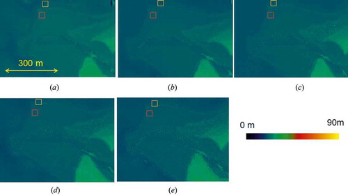
Table 2 shows that there are 29 interferometric pairs with five different incidence angles. Owing to the high latitude of this test site, many TDX passes can be acquired over short time intervals. A number of combinations of stereo pairs can be selected and several DEMs at the same incidence angle and different incidence angles can be averaged. Furthermore, the coherence is extremely high also in the pursuit mono-static mode of Tan DEM-X due to the cold and dry weather and little vegetation. Figure 5 shows a CoSSC staring spotlight image from 4 February 2015 in the region around Nikel. The ice-covered Pasvik hydropower lake can be seen to the left in the image. We selected a point-like target (G1) close to the nickel smelter as the GCP. We selected 13 stereo pairs from Table 2 and estimated the absolute height for each pair. The mean and standard deviation of the stereo heights were 91.65 m and 0.24 m, respectively. The interferogram from 4 February is shown in Figure 6. The mean coherence for this scene is 0.75. Figure 7 shows the UTM geocoded DEM using the StInSAR program. Figure 8 (a) shows a sub-image around the A1 point in Figure 5. Figure 8 (b) shows an averaged DEM generated from six DEMs with incidence angle 47º: 22 December, 2 January, 13 January, 4 February, 15 February, and 9 March in Table 2. The mean height in the A1 square in the left image is 41.15 m and the standard deviation is 0.98 m. The mean height in the A1 square in the averaged DEM in the right image is 40.70 m and the standard deviation is 0.41 m. This means that the standard deviation has been reduced from 0.98 m to 0.41 m. The averaged DEM looks smoother, especially in the dark regions, e.g. the roofs on the houses look much better. Figure 9 shows the averaged DEMs for five different incidence angles with squares drawn around the A2 and A3 points in Figure 5. If we take a new average in the squares of the five DEMs over different incidence angles, we obtain a mean height of 21.5 m and a standard deviation of 0.14 m in square A3, which is on land close to the hydropower lake. In square A2, which is on the shore, the absolute height is 21.0 m and the standard deviation is 0.12 m. In Norwegian maps, the height of the hydropower lake is 21.2 m; hence, there is only a few decimetres difference compared with the height estimated from the averaged StInSAR DEMs. The height of the hydro power lake in Norwegian maps is probably the height when excess water flows over the dam.

Figure 9. Averaged time series of DEMs at different incidence angles in a small region around the A2 and A3 points shown in Figure 5. The dates of the DEMs for each incidence angle are: (a) Incidence angle = 27°. Dates: 29 December, 9 January, 20 January, 11 February, 22 February. (b) Incidence angle = 35°. Dates: 23 December, 3 January, 14 January, 16 February, 27 February, 10 March. (c) Incidence angle = 41°. Dates: 17 December, 28 December, 8 January, 19 January, 10 February, 21 February. (d) Incidence angle = 47°. Dates: 22 December, 2 January, 13 January, 4 February, 15 February, 9 March. (e) Incidence angle = 52°. Dates: 16 December, 27 December, 7 January, 9 February, 20 February, 3 March.

4.3 Test site Åraksbø

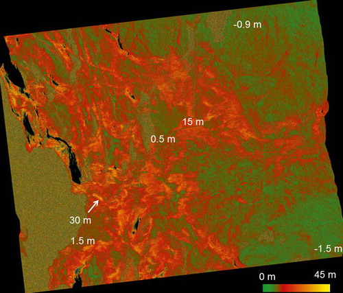
For this test site we used high-resolution spotlight images from both pursuit mono-static and bi-static modes at different incidence angles. The scenes are listed in Table 3. Åraksbø and Åraksfjorden lakes are shown in Figure 10, which is a photograph taken from powered paragliding. Figure 11 shows a sub-image of the bi-static spotlight image of 16 November 2015 in Table 3 over Åraksbø and a small part of Åraksfjorden lake. Scattered houses on small farms can be seen. The coherence images from the bi-static and mono-static modes are shown in Figure 12 (a) and (b), respectively. From Table 3, the average coherence of the bi-static images can be estimated to be 0.66 whereas the average coherence of the mono-static images is 0.55. The coherence in the bi-static images is substantially higher than in the mono-static images in some regions that are covered by mostly spruce and partly pine. A thorough evaluation of the TDX coherence during the bi-static Commissioning Phase can be found in Martone et al. (2012). Four GCPs are used as stereo points and are indicated with arrows (G1–G4) in Figure 12 (a). G1 and G4 are shown in Figures 10 and 11, respectively. G1 is a crossroad and G4 is some equipment for a tractor on the grassland. In this test site there are also five TPs that we use for the validation of height accuracy. Figure 13 shows the StInSAR DEM, which shows that the elevations vary from about 200 m close to the Åraksfjorden lake to the highest peak at 973 m in the upper right corner. Figure 14 shows the difference of the StInSAR DEM and the DTM from Norwegian mapping authority. If we compare Figures 12 and 14 we can see that the regions with lower coherence in the mono-static image also have larger heights, which indicate forest-covered areas. From Figures 13 and 14, it can be seen that the forest height is around zero when the elevations are larger than 700 m above the sea (areas with dark green, mixed with some red colour). The mean over a region in the upper right part of the image is −0.9 m. Here is almost no spruce and pine, only scattered birch. Close to the Åraksfjorden lake there is a region with a mean height of 30 m, which is an area covered with spruce. The farms in Åraksbø have a height of about 1.5 m.

Figure 10. Photograph taken by Johnny Foss over Åraksbø with powered paragliding on 19 July 2012 with licence from Norwegian airsport federation.

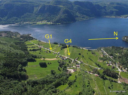
Figure 11. Bi-static spotlight image over Åraksbø on 16 November 2015 in Table 3.

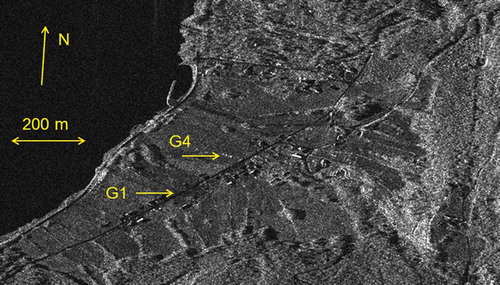
Figure 12. (a) Coherence of the bi-static image pair on 5 November 2015 in Table 3. Azimuth time difference of TSX and TDX is 0.03 s. (b) Coherence of the mono-static image pair of 21 December 2014 in Table 3. Azimuth time difference of TSX and TDX is 10 s.

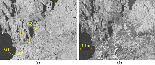
Figure 13. UTM geocoded DEM derived from the bi-static interferometric image pair of 16 November 2015 in Table 3. Pixel spacing is 2.0 m for the Northing and Easting. Scene centre: 58º 56ʹ 20ʺ N, 7º 47ʹ 2ʺ E.

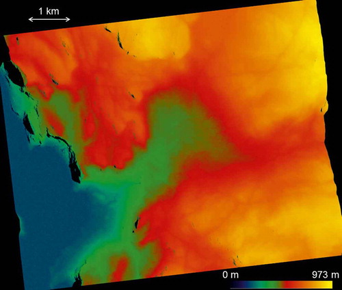
Figure 14. Difference of the DEM in Figure 13 and the DTM from NMA.

We use the height of one GCP as input to the absolute height estimation in the StInSAR DEM. Since CRs were not available in this test area, we used the three other GCPs and five TPs as reference points. Tables 8 and 9 show the estimated ME and RMSE for four mono-static and three bi-static scenes, respectively. The ME and RMSE are typically a few metres, which is quite a lot larger than at the test site Kjeller. The reason is that the TPs are located in a hilly and rugged terrain, which causes the heights to be somewhat underestimated (negative heights).

Table 8. Mean error (ME) and root mean square error (RMSE) in the four mono-static scenes from Table 3 using four stereo points and five trigonometric points as references.

	G1	G2	G3	G4
ME (m)	−3.05	−1.78	−1.91	−1.81
RMSE (m)	4.28	3.59	3.18	2.61

Table 9. Mean error (ME) and root mean square error (RMSE) in three bi-static scenes from Table 3 using four stereo points and five trigonometric points as references.

	G1	G2	G3	G4
ME (m)	−3.04	−0.25	−3.08	−2.08
RMSE (m)	4.58	3.20	4.36	3.63

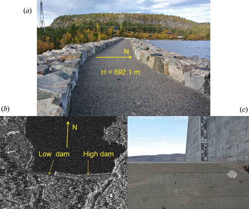
We used G1, G2, G3 and seven mono-static scenes in Table 3 and estimated the mean height (average over 3 x 7 heights) of the road upon a hydropower dam. The hydropower lake called Hovatn can be seen in the upper right part of the coherence images in Figure 12. The mean height was 691.68 m and the standard deviation was 0.67 m, which agrees very well with the measuring stick attached to the high dam. It shows 692.1 m on the road on top of the dam. Figure 15 (a) shows the road upon the dam and Figure 15 (c) shows the low and high dam with the measuring stick. Figure 15 (b) shows the low and high dam in the spotlight SAR image.

Figure 15. (a) Road upon the high hydropower dam. (b) SAR image showing low and high hydropower dam at Hovatn. (c) Low and high dam with the measuring stick. Photographs: Knut Eldhuset, October 2015.

5. Conclusions

We have used software developed at FFI for pixel location, stereo height estimation, InSAR processing, and DEM generation to estimate the absolute heights in TDX staring spotlight and high-resolution spotlight interferometric images from the scientific phase. The absolute height accuracy in the StInSAR-derived DEMs is only a few decimetres when the reference heights are selected on locally flat areas. In more rugged and hilly terrains, the heights are slightly underestimated with accuracies of a few metres.

Acknowledgement

This work was supported by the Norwegian Defence Research Establishment (FFI). We very much appreciate the kind help from the science team at DLR, Thomas Busche, and Irena Hansjek at DLR for the planning and delivery of CoSSC TanDEM-X data (AO-project NTI_INS6664). Thanks to Research Manager Richard B. Olsen at FFI and the anonymous reviewers for providing valuable comments to the manuscript.

Disclosure statement

No potential conflict of interest was reported by the author.

Additional information

Funding

This work was supported by the Norwegian Defence Research Establishment (FFI) [-].

References

- Avtar, R., A. P. Yunus, S. Kraines, and M. Yamamuro. 2015. “Evaluation of DEM Generation Based on Interferometric SAR Using Tandem-X Data in Tokyo.” Physics and Chemistry of the Earth 83-84: 166–177. doi:10.1016/j.pce.2015.07.007.
- Bachmann, M., J. H. Gonzales, G. Krieger, M. Schwerdt, J. W. Antony, and F. DeZan. 2012. “Calibration of the Bistatic Tandem-X Interferometer.” In Proceedings of the European Conference on Synthetic Aperture Radar (EUSAR 2012). Nuremberg, Germany. 23-26 April 2012.
- Balss, U., H. Breit, S. Duque, T. Fritz, and C. Rossi. 2014. “Payload Ground Segment: CoSSC Generation and Interferometric Considerations.” [Online] Available: https://tandemx-science.dlr.de/pdfs/TD-PGS-TN-3129_CoSSCGenerationInterferometricConsiderations_1.0.pdf
- Eldhuset, K., P. H. Andersen, S. Hauge, E. Isaksson, and D. J. Weydahl. 2003. “ERS Tandem Insar Processing for DEM Generation, Glacier Motion Estimation and Coherence Analysis on Svalbard.” International Journal of Remote Sensing 24: 1415–1437. doi:10.1080/01431160210153039.
- Eldhuset, K., and D. J. Weydahl. 2011. “Geolocation and Stereo Height Estimation Using Terrasar-X Spotlight Image Data.” IEEE Transactions on Geoscience and Remote Sensing 49: 3574–3581. doi:10.1109/TGRS.2011.2160951.
- Eldhuset, K., and D. J. Weydahl. 2013. “Using Stereo SAR and Insar by Combining the COSMO-Skymed and Tandem-X Mission Satellites for Estimation of Absolute Height.” International Journal of Remote Sensing 34: 8463–8474. doi:10.1080/01431161.2013.843808.
- Gisinger, C., U. Balss, R. Pail, X. Xiang Zhu, S. Montazeri, S. Gernhardt, and M. Eineder. 2015. “Precise Three-Dimensional Stereo Localization of Corner Reflectors and Persistent Scatterers with Terrasar-X.” IEEE Transactions on Geoscience and Remote Sensing 53: 1782–1802. doi:10.1109/TGRS.2014.2348859.
- Gonzáles, J. H., M. Bachmann, G. Krieger, and H. Fiedler. 2010a. “Development of the Tandem-X Calibration Concept: Analysis of Systematic Errors.” IEEE Transactions on Geoscience and Remote Sensing 48: 716–726. doi:10.1109/TGRS.2009.2034980.
- González, J. H., M. Bachmann, R. Scheiber, and G. Krieger. 2010b. “Definition of Icesat Selection Criteria for Their Use as Height References for Tandem-X.” IEEE Transactions on Geoscience and Remote Sensing. 48: 2750–2757. doi:10.1109/TGRS.2010.2041355.
- Gruber, A., B. Wessel, M. Martone, and A. Roth. 2016. “The Tandem-X DEM Mosaicking: Fusion of Multiple Acquisitions Using Insar Quality Parameters.” IEEE Journal of Selected Topics in Applied Earth Observations and Remote Sensing 9: 1047–1057. doi:10.1109/JSTARS.2015.2421879.
- Hajnsek, I., T. Busche, G. Krieger, M. Zink, D. Schulze, and A. Moreira. 2014. “Announcement of Opportunity: TanDEM-X Science Phase.” Available online at: https://tandemx-science.dlr.de/pdfs/TD-PD-PL_0032TanDEM-X_Science_Phase.pdf
- Kraus, T., B. Bräutigam, J. Mittermayer, S. Wollstadt, and C. Grigorov. 2016. “Terrasar-X Staring Spotlight Mode Optimization and Global Performance Predictions.” IEEE Journal of Selected Topics in Applied Earth Observations and Remote Sensing 9: 1015–1027. doi:10.1109/JSTARS.2015.2431821.
- Krieger, G., A. Moreira, H. Fiedler, I. Hajnsek, M. Werner, M. Younis, and M. Zink. 2007. “Tandem-X: A Satellite Formation for High-Resolution SAR Interferometry.” IEEE Transactions on Geoscience and Remote Sensing 45: 3317–3340. doi:10.1109/TGRS.2007.900693.
- Krieger, G., M. Zink, M. Bachmann, B. Bräutigam, D. Schulze, M. Martone, P. Rizzoli, et al. 2013. “Tandem-X: A Radar Interferometer with Two Formation-Flying Satellites.” Acta Astronautica 89: 83–98. doi:10.1016/j.actaastro.2013.03.008.
- Lachaise, M., and T. Fritz. 2016. “Update of the Interferometric Processing Algorithms for the Tandem-X High Resolution Dems.” In Proceedings of the European Conference on Synthetic Aperture Radar (EUSAR 2016), 6-9 June 2016. Hamburg, Germany: VDE VERLAG GMBH.
- Martone, M., B. Bräutigam, P. Rizzoli, C. Gonzales, and M. Bachmann. 2012. “Coherence Evaluation of Tandem-X Interferometric Data.” ISPRS Journal of Photogrammetry and Remote Sensing 73: 21–29. doi:10.1016/j.isprsjprs.2012.06.006.
- Mittermayer, J., S. Wollstadt, P. Prats-Iraola, and R. Scheiber. 2014. “The Terrasar-X Staring Spotlight Mode Concept.” IEEE Transactions on Geoscience and Remote Sensing 52: 6003–6016. doi:10.1109/TGRS.2013.2274821.
- Norwegian Mapping Authority (NMA). 2014. Available online at http://www.kartverket.no/en/data/Open-and-Free-geospatial-data-from-Norway/( accessed 22 September 2014).
- Norwegian Mapping Authority (NMA). 2016. Available online at: http://www.norgeskart.no/fastmerker/#5/378604/7226208 ( accessed 18 October 2016).
- Prats-Iraola, P., R. Scheiber, M. Rodriguez-Cassola, J. Mittermayer, S. Wollstadt, F. De Zan, B. Bräutigam, M. Schwerdt, A. Reigber, and A. Moreira. 2014. “On the Processing of Very High Resolution Spaceborne SAR Data.” IEEE Transactions on Geoscience and Remote Sensing. 52: 6003–6016. doi:10.1109/TGRS.2013.2294353.
- Rizzoli, P., B. Bräutigam, T. Kraus, M. Martone, and G. Krieger. 2012. “Relative Height Error Analysis of Tandem-X Elevation Data.” ISPRS Journal of Photogrammetry and Remote Sensing 73: 30–38. doi:10.1016/j.isprsjprs.2012.06.004.
- Rossi, C., F. R. Gonzales, T. Fritz, N. Yague-Martinez, and M. Eineder. 2012. “Tandem-X: Calibrated Raw DEM Generation.” ISPRS Journal of Photogrammetry and Remote Sensing 73: 12–20. doi:10.1016/j.isprsjprs.2012.05.014.
- Tridon, D. B., M. Bachmann, D. Schulze, M. D. Polimeni, M. Martone, J. Böer, and M. Zink. 2014. “Tandem-X DEM Difficult Terrain & Antarctica Acquisitions Towards the Planning of the Science Phase.” In Proceedings of the European Conference on Synthetic Aperture Radar (EUSAR 2014), 3-5 June 2014. Berlin, Germany: VDE VERLAG GMBH.
- Viewfinder Panoramas, Available online at http://viewfinderpanoramas.org/dem3.html ( accessed 26 May 2014).
- Wecklich, C., C. Gonzalez, B. Bräutigam, and P. Rizzoli. 2016. “Height Accuracy and Data Coverage Status of the Global Tandem-X DEM.” In Proceedings of the European Conference on Synthetic Aperture Radar (EUSAR 2016), 6-9 June 2016. Hamburg, Germany: VDE VERLAG GMBH.
- Wessel, B., M. Breunig, M. Bachmann, M. Huber, M. Martone, M. Lachaise, T. Fritz, and M. Zink. 2016. “Concept and First Example of Tandem-X High Resolution DEM.” In Proceedings of the European Conference on Synthetic Aperture Radar (EUSAR 2016), 6-9 June 2016. Hamburg, Germany: VDE VERLAG GMBH.