Subpixel land-cover classification for improved urban area estimates using Landsat

ABSTRACT

Urban areas are Earth’s fastest growing land use that impact hydrological and ecological systems and the surface energy balance. The identification and extraction of accurate spatial information relating to urban areas is essential for future sustainable city planning owing to its importance within global environmental change and human–environment interactions. However, monitoring urban expansion using medium resolution (30–250 m) imagery remains challenging due to the variety of surface materials that contribute to measured reflectance resulting in spectrally mixed pixels. This research integrates high spatial resolution orthophotos and Landsat imagery to identify differences across a range of diverse urban subsets within the rapidly expanding Perth Metropolitan Region (PMR), Western Australia. Results indicate that calibrating Landsat-derived subpixel land-cover estimates with correction values (calculated from spatially explicit comparisons of subpixel Landsat values to classified high-resolution data which accounts for over [under] estimations of Landsat) reduces moderate resolution urban area over (under) estimates by on an average 55.08% for the PMR. This approach can be applied to other urban areas globally through use of frequently available and/or low-cost high spatial resolution imagery (e.g. using Google Earth). This will improve urban growth estimations to help monitor and measure change whilst providing metrics to facilitate sustainable urban development targets within cities around the world.

1. Introduction

Urban areas are estimated to cover only 0.5% of Earth’s surface yet are one of the fastest growing land use per area basis (Schneider, Friedl, and Potere 2010; Bettencourt and West 2010; Schneider, Friedl, and Potere 2009). Population growth has resulted in increased urbanization with 54% of the planet’s seven billion people in 2014 residing in urban areas with an additional 2.5 billion urban dwellers projected by 2050, whilst concurrently increasing the proportion of world’s urban population to 66% (Sexton et al. 2013; Powell and Roberts 2010; Sharifi and Lehmann 2014; United Nations, Department of Economic and Social Affairs, Population Division 2014; Powell et al. 2007; Song et al. 2016). Alteration of natural land cover to anthropogenic impervious surfaces has been identified as the most extreme cumulative effect of land-cover change, generating numerous socio-economic consequences including amenity provision efficiency, ecological degradation, and the Urban Heat Island (UHI) effect (Cai et al. 2016; Howard 1988; L. Hu and Brunsell 2015; Xie and Zhou 2015). Accurate information on urban Land Cover and Land Use (LULC) is therefore imperative for monitoring expansion and planning policy targeting for future sustainable development of our cities (Bettencourt and West 2010; Wu and Murray 2003). Earth Observation (EO) enables consistent, detailed characterization of the actual urban footprint of a city having been mapped and monitored using remotely sensed data at a range of spatial and temporal scales for associated implications (Schneider, Friedl, and Potere 2010; Imhoff et al. 1997; Sexton et al. 2013; Akbari, Rose, and Taha 2003; Friedl et al. 2002). However, accurate and consistent monitoring of urban land cover is frequently precluded by coarse spatial (e.g. 1 km² Moderate Resolution Imaging Spectroradiometer (MODIS) land-cover product) and temporal (e.g. 2000 and 2010 GlobeLand30 product) resolution of such data sets (Song et al. 2016; Lu et al. 2014).

Urban mapping remains challenging due to the heterogeneity of surface materials and surface structure which contributes to pixel surface reflectance that are often difficult to disentangle (Herold et al. 2002; Lu, Moran, and Hetrick 2011; Varshney and Rajesh 2014; Schneider 2012). When delineating urban land cover from remotely sensed data, spatial resolution is considered the most important factor that provides increased visibility of discrete surface features (e.g. buildings) and greater pixel homogeneity over medium to coarse spatial resolution satellite imagery (e.g. Landsat and MODIS) (Myint et al. 2011). Nevertheless, high spatial resolution data often lack temporal acquisition consistency (e.g. airborne orthophotos) or are expensive to purchase (e.g. commercial satellite imagery). Consequently, in order to best monitor urban LULC change, data sets must have an adequate spatial and temporal resolution to discern change. In this regard, data from the Landsat series of satellites provide the longest time-series of consistent, medium spatial resolution imagery that has been extensively applied to urban area mapping (Powell et al. 2007; Schneider and Mertes 2014; Sundarakumar et al. 2012; Wilson et al. 2003; Yuan et al. 2005; Song et al. 2016).

Accurate quantification of anthropogenic landscape modification is of critical importance due to associated environmental, anthropogenic, and climatic impacts (Kalnay and Cai 2003). Urban estimates from Landsat data have been used within global biogeochemistry and climate models (Z. Zhu and Woodcock 2014), further scientific studies such as UHI investigations (Y. Hu et al. 2015) and targeted urban development policies (Schneider, Seto, and Webster 2005; Hepinstall-Cymerman, Coe, and Hutyra 2013). Whilst comparative studies (e.g. Li et al. 2014) have shown marginal holistic image accuracy difference between algorithm selection on per-pixel Landsat classification assuming sufficient training data, traditional per-pixel methods, such as the Maximum Likelihood Classifier (discussed in supplementary Section 1), have been found to significantly over or underestimate urban area from Landsat data (Lu, Moran, and Hetrick 2011; Wu and Murray 2003). Addressing this error is important when accurate classifications are required for monitoring change in land-use patterns whereby calculations of urban extent can influence decision-making (e.g. policy for sustainable urban development) (Schneider, Seto, and Webster 2005; Hepinstall-Cymerman, Coe, and Hutyra 2013; Miller and Small 2003; Bagan and Yamagata 2014).

Due to the heterogeneity of urban areas, subpixel classification methodologies have been increasingly applied to medium spatial resolution data to more accurately represent the mixture of land covers within a pixel (Lu, Moran, and Hetrick 2011; Lu and Weng 2006; Powell and Roberts 2008; Weng and Ruiliang 2013; Wang et al. 2013). This has been achieved through variations of spectral mixture analysis (SMA) where a set number of representative endmembers, frequently following the Vegetation, Impervious and Soil (V-I-S) framework, are used to model the entire image based on their spectral characteristics (Powell et al. 2007; Ridd 1995). However, endmembers may not fully represent image spectral variability or a pixel may be modelled by endmembers that do not represent materials within its field of view resulting in an inability to adequately portray the high spectral heterogeneity of the urban landscape (Powell et al. 2007). Support Vector Machine (SVM) spectral unmixing attempts to resolve this issue through consideration of a large number of training pixels which provides preferential accuracy in comparison to SMA although high dimensional data and large training samples can hinder its performance (Wang et al. 2013).

Comparatively, the novel sub and hard pixel Import Vector Machine (IVM) classifier permits simultaneous multi-class comparison whilst continuously testing training samples for validity providing a more accurate solution (Roscher, Förstner, and Waske 2012). IVM has been found to consistently outperform decision trees, artificial neural networks, and maximum likelihood algorithms (Watanachaturaporn, Arora, and Varshney 2008; Kotsiantis, Zaharakis, and Pintelas 2006; Huang, Davis, and Townshend 2002), with preferential (Braun, Weidner, and Hinz 2012) and comparable results to SVM (Roscher, Waske, and Forstner 2010). However, due to the heterogeneity of urban areas, it is important to calibrate these subpixel approaches against high spatial resolution data that capture the diverse characteristics found within urban environments (Lu, Moran, and Hetrick 2011). Perth, Western Australia (WA), is characterized by extensive urban diversity, surpassing all other major Australian and US cities in terms of suburban development (Kelly, Weidmann, and Walsh 2011; U.S. Department of Commerce 2013). It therefore provides a suitable case study for assessing the ability of Landsat to map urban development, which is a prerequisite for appropriate policy incorporation. This article describes an approach to map the urban extent of the Perth Metropolitan Region (PMR) using an IVM classifier applied to medium spatial resolution imagery. The impact of subpixel land-cover heterogeneity is investigated by comparing the urban area estimates to those derived from very high spatial resolution (20 cm) imagery. An innovative, spatially explicit correction to account for over (or under) estimation of urban area is derived which improves the urban land-cover estimates from medium resolution imagery.

2. Study area

The PMR (Figure 1(a)), WA, has experienced sustained urban development since the twenty-first century in response to a rapidly growing resource sector (Kennewell and Shaw 2008). The majority of recent urban growth within the PMR has transpired as outward low-density development resulting in a maximum population density of 3662 km² which is 33.45% and 24.83% lower than Melbourne (10,827) and Sydney (14,747), respectively (Western Australian Planning Commission 2015; ABS 2015). The notion of the ‘Australian dream,’ depicted as detached living in a green suburb, is most pronounced in Perth (Western Australian Planning Commission 2013a). As a result, 79% of the current housing is detached, compared to 62% in Sydney, 72% in Melbourne, and a national average of 74% (Kelly, Weidmann, and Walsh 2011; Western Australian Planning Commission 2013b). Globally, Australia surpasses other developed countries in terms of detached suburban living with UK having 42% of housing as either detached or semi-detached (Department for Communities and Local Government 2015). Similarly, only 64.2% of USA housing stock is detached, with Perth eclipsing all of the major 25 USA metropolitan areas in terms of detached housing (U.S. Department of Commerce 2013). Low population density and outward expansion witnessed in Perth have generated high demand for dispersed amenities and services in a non-strategic, ‘lot-by-lot fashion’ (Dhakal 2014). Suburbanization of this nature has been identified as unsustainable due to impacts on ecological systems (e.g. habitat fragmentation) and socio-economic issues (e.g. amenity provisioning costs), with accurate urban area identification essential for sustainable future planning and maximum resource efficiency, particularly in Perth owing to its globally high suburbanization and distributed population (Western Australian Planning Commission 2013a).

Figure 1. Landsat 8 operational land imager (OLI) true colour image mosaic of the Perth Metropolitan Region (9 August 2015 [path 112] and 17 September 2015 [path 113]). The locations of the high spatial resolution aerial image subsets are indicated by coloured overlays (a), with Western Australia identified in (b) and Perth city (c).

Therefore, the PMR provides a globally diverse range of urban characteristics (e.g. compact urban central business district, older residential areas, and new suburban developments) facilitating broad data set comparison opportunities between Landsat and high spatial resolution urban area estimates. The high spatial resolution data identify the complexity of these suburban and urban areas, which is obscured in medium and coarse spatial resolution data sets. This permits the extraction of individual features such as buildings, roads, and vegetation that compose the urban environment and which are represented as a spectrally mixed pixel in Landsat imagery (illustrated in Figure 2) (Myint et al. 2011).

Figure 2. Comparison of true colour high spatial resolution data (a) (acquired from 14 March 2007) and Landsat surface reflectance (b) (acquired on 6 October 2007 [path 112]), highlighting the spatial detail captured by high-resolution imagery (c) and the same areas as observed by Landsat (d) for the subset East Beechboro used within this study.

Definitive feature detection from high-resolution data can assist in refining urban area estimates produced from moderate spatial resolution satellite imagery (Lu, Moran, and Hetrick 2011; Wu and Murray 2003). More accurate satellite-derived urban area estimates are imperative for ensuring appropriate data use for policy and environmental variable applications in order to mitigate the consequences of unsustainable urban development. This aligns with the criteria of effective land-use planning within the City Resilience Framework that is designed to improve city resilience (ARUP, and The Rockefeller Foundation 2015).

3. Data

3.1. Landsat data

Cloud-free Landsat scenes were obtained for 2007 from Landsat 5 Thematic Mapper (TM), coinciding with high-resolution orthophotos (described in Section 3.2). Imagery was acquired within winter months (9 July 2007 for path 113 and 6 October 2007 for path 112) corresponding with peak vegetation green-up which limits issues concerning the spectral separation between senescent vegetation, bare earth, and some impervious surfaces (Feyisa et al. 2016; Chen et al. 2014). Landsat imagery was processed to standard terrain correction (Level 1T), geometrically and topographically corrected using ground control points and a digital elevation model from the Global Land Survey 2000 data set (Hansen and Loveland 2012). Landsat 5 TM surface reflectance values were derived from the Landsat Ecosystem Disturbance Adaptive Processing System (Hansen and Loveland 2012; Jeffrey G. Masek et al. 2006) which corrects for atmospheric effects using the Second Simulation of a Satellite Signal in the Solar Spectrum (6S) radiative transfer model (Vermote et al. 1997).

3.2. High spatial resolution airborne imagery

Radiometrically calibrated multispectral red (0.58–0.77 µm), green (0.48–0.63 µm), blue (0.41–0.54 µm), and near-infrared (0.69–1.00 µm) orthophotos were acquired over 19 cloud-free days commencing on 14 March 2007 as part of the Perth and Peel Urban Monitor Programme (Caccetta et al. 2012). Aerial imagery, obtained between 10:00 and 14:00 to reduce shadow effects, was captured using a Microsoft UltraCAM-D at a height of 1300 m resulting in a spatial resolution of 20 cm. Forward and side frame overlap of 60% and 30%, respectively, permitted automatic digital surface model (DSM) extraction using geometric control points provided by WA’s land information authority (Landgate). Extraction of ground points exclusively representing terrain variations facilitated derivation of a Ground Elevation Model which, when subtracted from the DSM, generated a Relative Elevation Model, depicting elevation relative to ground points.

Spatial and temporal inconsistencies in reflectance can arise from atmospheric scattering and absorption, instrument noise and Bidirectional Reflection Distribution Function (BRDF) effects. The latter describes the systematic variation in reflectance across an image due to differences in view and illumination angles and which is dependent on the surface 3D structure (Collings, Caccetta, and Campbell 2011). The orthophotos were provided as a surface reflectance product, corrected for multiplicative and additive errors over frames (e.g. instrument noise and atmospheric effects) and within frame viewing and illumination geometry (Caccetta et al. 2012; Collings, Caccetta, and Campbell 2011). Image preprocessing consisted of two steps. First, a combined BRDF and atmospheric correction procedure was applied to retrieve surface reflectance for each image acquisition. Linear BRDF model parameters from the Li Sparse reciprocal kernel (Wanner, Li, and Strahler 1995) were used to correct for BRDF effects. Atmospheric perturbations were corrected by assuming that the obtained digital number represented the relative reflectance affected by spatially dependent multiplicative and additive terms. These combined steps generated an internally consistent mosaicked data set. ‘True’ surface reflectance was estimated through fitting global offset and gain values to replicate laboratory measured calibration targets based on the assumption that relative reflectance requires a linear transformation to true reflectance (Collings, Caccetta, and Campbell 2011).

4. Methodology

4.1. Landsat preprocessing

The two Landsat scenes covering the study area were combined to form a seamless image mosaic following the methodology of Pan et al. (2009). Voroni diagrams were created on the bisector between images with adjacent edges defined as seamlines, identifying effective mosaic polygons that specify pixels from each image to include in the final mosaic, facilitating less visible boundaries through blending of overlapping pixels (Pan et al. 2009) (Figure 1(a)). Due to remaining residual noise in the mosaicked imagery caused by factors such as the brightening effect of thin clouds and atmospheric correction differences, surface reflectance values were standardized following the approach identified by Sexton et al. (2013):

(1) $p_{i,\mathrm{b}}=\frac{p_{x,\mathrm{b}}}{\mathrm{m}\mathrm{a}{\mathrm{x}}_{\mathrm{b}}}$(1)

where $p_{i,\mathrm{b}}$ is the standardized pixel value $\hspace{0.17em}i$, from band $\mathrm{b}$ based on the original surface reflectance $x$, standardized through division by a waveband-specific upper reflectance limit which are 0.10 (blue; 0.48 µm), 0.11 (green; 0.56 µm), 0.12 (red; 0.66 µm), 0.23 (near-infrared; 0.84 µm), 0.21 (shortwave infrared; 1.65 µm), 0.15 (shortwave infrared 2; 2.22 µm). The standardized values ($p_{i,\mathrm{b}}$) were then normalized against the summed band standardized values:

(2) $p_{j,\text{b}}=\frac{p_{i,\text{b}}}{\sum i{p}_{i,\text{b}}}$(2)

where $\sum _i{p}_{i,\mathrm{b}}$ is the sum of each standardized pixel across all bands (Sexton et al. 2013). This approach has been found to satisfactorily reduce variations generated from inherent residual noise across mosaicked imagery, for example due to differences in modelled atmospheric parameters within the LEDAPS algorithm (Sexton et al. 2013; Luo et al. 2014) (Figure 3(a)). Statistical assessment of image radiometric normalization provided in MacLachlan et al. (2017a) found that the post-processed Landsat data exhibited significantly lower inter- and intra-coefficient of variation when compared to the preprocessed data.

Figure 3. Summary of classification procedures for (a) Landsat and (b) high-resolution orthophoto data.

4.2. Landsat classification

The 2007 Landsat data were classified as a time series of data for seven sequential periods between 1990 and 2015 using an IVM classifier produced in MacLachlan et al. (2017a). The method uses a hybrid strategy that assesses whether new samples (termed import vectors) can be removed in each forward step in order to provide a smoother decision boundary that ideally leads to a more accurate solution (Roscher, Förstner, and Waske 2012). Samples are selected based on how much their incorporation decreases the objective function to minimize the decision boundary to form the optimal separating hyperplane between overlapping clusters (e.g. land-cover types) in spectral feature space (Mountrakis, Jungho, and Ogole 2011; Roscher, Förstner, and Waske 2012; J. Zhu and Hastie 2005). IVM generates two outputs: a soft (subpixel) data set that defines the probability of a pixel containing a given classification value (e.g. land-cover type) and a traditional ‘hardened’ classified data set (Braun, Weidner, and Hinz 2012). Training samples were collected from the 12 and 19 July 2005 Landsat 5 TM image composite, coinciding with peak vegetation greenness which provides the greatest spectral separability between vegetated and non-vegetated surfaces (Feyisa et al. 2016; Chen et al. 2014). Six land-cover types were defined based on existing literature (e.g. X. Hu and Weng 2009; Schneider 2012; Feyisa et al. 2016) and scene analysis which are high reflectance urban (e.g. concrete), low reflectance urban (e.g. asphalt), forest, water, grassland, and bare earth. Two urban land-cover classes are specified to reduce spectral confusion between spectrally similarly classes (e.g. urban and bare earth) (X. Hu and Weng 2009). For each land-cover type, 250 pixels were randomly identified from across the image for training the IVM classifier that follows the approach used by Foody and Mathur (2006) and Pal and Mather (2003). The IVM algorithm is parameterized using the training data that generate a classification model consisting of spectral profiles for each land-cover type, which are then matched to the Landsat mosaic during classification.

The resulting per-pixel (hardened) classification indicates that the total urban extent of the PMR has increased 45.32% (subpixel estimate of 32.96%) between 1990 (hardened estimate 706.88 km², subpixel estimate 736.93 km²) and 2015 (hardened estimate 1027.22 km², subpixel estimate 979.84 km²) (MacLachlan et al. 2017a). This can be broken down into low reflectance urban cover expanding from a hardened value of 592.83 km² (subpixel estimate 668.46 km²) to 839.00 km² (subpixel estimate 850.87 km²) and high reflectance urban cover increasing from a hardened value of 114.05 km² (subpixel estimate 135.32 km²) to 188.20 km² (subpixel estimate 214.06 km²) across the same temporal period.

4.3. Google Earth Landsat accuracy assessment

Google Earth imagery consistent with the Landsat acquisition date was used to assess the accuracy of the hardened Landsat classification following previously published methods (e.g. Dorais and Cardille 2011; Cunningham et al. 2015; Song et al. 2016; Sun et al. 2015; Bagan and Yamagata 2014; Z. Zhu and Woodcock 2014). Using the Google Earth imagery, 300 random locations (50 per land-cover class) within the PMR were visually identified and compared to the classified land-cover data, consistent with recommended land-cover accuracy sample size of Congalton (2001) (Song et al. 2016). The 2007 Landsat classification obtained an accuracy of 84.00% and a kappa coefficient of 0.78. Urban land-cover estimates had a producer’s accuracy of 83.00% and user’s accuracy of 87.37%. MacLachlan et al. (2017a) provide a full breakdown of urban temporal change and associated accuracy for all imagery in the Landsat time series (1990–2015), with the Landsat classification data available from the pangea open access publisher (DOI: 10.1594/PANGAEA.871017) (MacLachlan et al. 2017b).

4.4. Aerial image classification

Urban areas are complex, heterogeneous environments that are challenging to classify even when using high spatial resolution multispectral imagery (Varshney and Rajesh 2014; Lu, Moran, and Hetrick 2011). Within urban areas, traditional moderate and coarse spatial resolution pixel-based classification methods present multiple challenges due to the land surface spatial heterogeneity and the spectral similarity between urban and non-urban materials (Myint et al. 2011). To characterize the influence of spatial resolution on the ability to map urban areas, high spatial resolution multispectral ortho-imagery (20 cm) was classified into the four broad land-cover types. To reduce data processing requirements, four 3 km² subsets were chosen which are representative of the land-cover composition and spatial heterogeneity found within Perth (Figure 1(a)). These subsets are an out of town development area (East Beechboro), the Central Business District (CBD), an older suburban area (Palmrya, Melville), and a largely vegetated region (Keysbrook). Using the high spatial resolution multispectral imagery and a relative elevation model, an Object Based Image Analysis (OBIA) method was applied to classify each subset into vegetation, urban, bare earth, and water (Figure 3(b)). OBIA methods are often applied to high spatial resolution imagery as they include spatial, textural, and spectral information to classify the scene (Myint et al. 2011). Incorporating surface elevation measurements into urban classifications has been found to improve building (urban) extraction accuracy (Aguilar et al. 2012; Poznanska, Bayer, and Bucher 2013). Surface elevation estimates and normalised difference vegetation index data provided additional urban classification parameters, with refinement (e.g. additions and alterations) made based on object spatial, spectral, and textural properties. Unlike the Landsat imagery, the airborne imagery was collected during the late dry season when the grass was senescent which resulted in textural and spectral similarity between bare earth and roads. To mitigate the impact of potential misclassification between these features, Landgate road and, where appropriate, rail vector data set was used for identification of coincident image objects for urban assignment.

4.5. Data set comparison and Landsat refinement

In order to compare the orthophoto and Landsat land-cover classifications, the two urban (high and low reflectance) and two vegetation (woodland and grassland) Landsat land-cover classes were merged so that both land-cover classifications contained four identical classes. To facilitate comparison between the high spatial resolution orthophoto-derived classification and the Landsat classification, the orthophoto land-cover data are aggregated to Landsat spatial resolution to provide a ‘soft’ and a ‘hard’ land-cover data set. To create the soft 30 m² orthophoto-derived classification, each resampled 30 m² pixel area contains the proportion of each land-cover type within it (Lu, Moran, and Hetrick 2011) (Figure 3(b)). This data set was subsequently ‘hardened’ by assigning the pixel land-cover type according to the dominant land cover found within the 30 m² area.

The comparison methodology is to first compare the per-pixel (i.e. hardened) Landsat land-cover classification with the aggregated (30 m²) orthoimage classification. Misclassified Landsat pixels are assessed further to establish the conditions that lead to erroneous classification using the subpixel proportion information (i.e. soft classification data sets). The latter are also used to identify a spatially explicit correction model to improve urban area estimates from moderate spatial resolution imagery.

5. Results

5.1. Orthophoto and Landsat land-cover comparison

A comparison is conducted between the orthophoto land-cover classification, aggregated to 30 m² spatial resolution using the majority land cover, and the IVM ‘hardened’ Landsat classification. At its native spatial resolution (20 cm; Figures 4(a–d(i))), the orthophoto land-cover classification (Figures 4(a–d(ii))) captures the land-cover spatial heterogeneity found within each region and highlights the difference in the spatial structure between these regions.

Figure 4. (i) High spatial resolution true colour orthophotos, (ii) land-cover maps, and (iii) the agreement between the orthophoto classification resampled to 30 m² and the Landsat classification for: (a) an out of town development area (East Beechboro), (b) old inner city urban area (central business district), (c) older suburban area (Palmrya, Melville), and (d) predominantly vegetated site (Keysbrook). In (iii), areas depicted as ‘true’ indicate those 30 m² pixels where the orthophoto land-cover type, based on the dominant land cover in the 30 m² area, and Landsat land-cover type are in agreement.

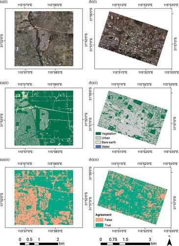
Figure 4. (Continued).

A comparison is carried out between the orthophoto land-cover classification, aggregated to 30 m² spatial resolution, and the ‘hardened’ Landsat classification. Figure 4(iii) illustrates the spatial agreement between these data sets and highlights those pixels where the same land-cover type (true) has been assigned to a pixel in both classifications. The areas that are more homogeneous at Landsat’s spatial resolution, such as the CBD (urban, Figure 4(b)) and Keysbrook (vegetation, Figure 4(d)), have greater level of agreement (73.14% and 95.68%, respectively). In contrast, the more heterogeneous subsets (East Beechboro and Palmrya, Figures 4(a,c)) have much lower levels of agreement (56.09% and 32.03%, respectively). The differences in agreement result from the subpixel heterogeneity at 30 m² spatial resolution. Table 2 shows the percentage of Landsat pixels which contain >50% of a given land-cover for each subset region.

Table 1. The percentage of different land-cover types within the classified high spatial resolution subsets (Figure 1).

Subset	Vegetation (%)	Urban (%)	Bare earth (%)	Water (%)
East Beechboro	81.00	16.56	2.37	0.07
CBD	33.33	65.66	0.91	0.10
Palmrya	57.29	42.21	0.42	0.08
Keysbrook	97.36	0.90	1.56	0.18

Table 2. The percentage of pixels which contain >50% of a given land-cover type in each region.

Subset	Vegetation (%)	Urban (%)	Bare earth (%)	Water (%)
East Beechboro	87.57	9.84	1.89	0.06
CBD	26.14	72.81	0.74	0.05
Palmrya	66.71	32.33	0.21	0.07
Keysbrook	98.90	0.05	0.88	0.11

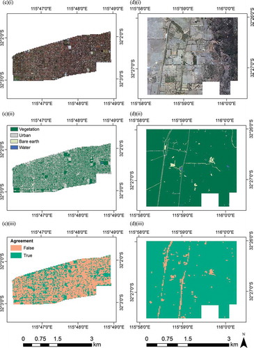
To investigate the influence of subpixel heterogeneity on the ability of Landsat to identify the pixel land-cover type, the classification accuracy is determined as a function of the percentage of urban area within each Landsat pixel for all four subsets (Figure 5). The urban percentage cover within each Landsat pixel is derived from the orthophoto land-cover classification that has been aggregated to 30 m² and that provides the proportion of each land cover within each pixel. The accuracy of the hardened Landsat classification was determined through comparison against the ‘hardened’ (e.g. aggregated to 30 m²) orthophoto land-cover classification where the per-pixel land-cover type was determined based on the land-cover type with the greatest subpixel proportion. Figure 5 indicates that the hardened Landsat classification results in a relatively high accuracy, with an average of 85.40% (excluding Keysbrook), for pixels containing >50% urban land cover (according to the high spatial resolution land-cover classification). In the subsets of East Beechboro, the CBD, and Palmrya, the overall Landsat classification accuracy drastically declines to 1.99–6.21% when urban land cover within a 30 m² pixel area decreases to 40–50%. The classification accuracy then increases with decreasing subpixel urban cover which is particularly evident with Landsat pixels containing 0–10% urban cover. Keysbrook, on the other hand, is a largely vegetated region and exhibits lower accuracy with increasing urban land cover.

Figure 5. Landsat classification accuracy as a function of the percentage urban cover within Landsat image pixels (as derived from the high spatial resolution land-cover data set) for each of the four subsets. In the Keysbrook subset, no Landsat pixels contained >60% urban land cover.

In order to understand the counter-intuitive behaviour of such as rapid decrease in classification accuracy in pixels which contain between 40% and 50% urban area (Figure 5), an analysis of the percentage of pixels classified as a given land-cover type is presented. To do so, all pixels containing different ranges in urban percentage cover (e.g. 0–10%, 20–30%, etc.) were identified using the high spatial resolution land-cover data set. The total percentage of each land-cover type was calculated for all pixels that contained urban percentage cover within each range urban percentage cover (e.g. 0–10%, 20–30%, etc.) using hardened IVM Landsat land-cover data set and the aggregated high spatial resolution land-cover data set (i.e. defined by the dominant land-cover type within a 30 m² pixel area).

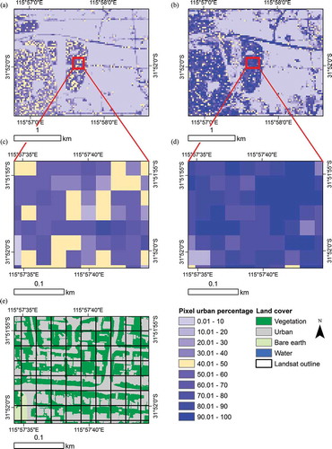
Figure 6 illustrates the percentage of pixels identified as a given land-cover type as indicated by the hardened Landsat land-cover data set and the hardened high spatial resolution orthophoto land-cover data set for pixels which contain differing percentage urban cover (e.g. 0–10%) derived using the original high spatial resolution orthophoto land-cover classification for the East Beechboro subset. This area was selected as it is an intermediate area in terms of land-cover heterogeneity (Figures 2 and 4(a)). The results indicate that the hardened Landsat classification consistently overestimates urban land cover when compared to the ‘hardened’ high spatial resolution classification which has been aggregated to 30 m² based on the dominate land cover within the Landsat pixel area for pixels with 10–50% urban defined by high-resolution data. Table 3 and Figure 7 illustrate the subpixel (30 m²) percentage urban land cover for East Beechboro with the original reflectance imagery for this area shown in Figure 2. The hardened high spatial resolution land-cover data set (left bar in each plot [Figure 6]) indicates that pixels containing <50% urban land cover are largely dominated by vegetation. In contrast, Landsat largely identifies these pixels as being either urban or vegetated to differing extents and more correctly identifies pixels with 0–10% urban land cover as being predominantly vegetated. For example, pixels containing 40–50% urban area are correctly identified as being vegetated (98.45% of pixels within this range) by the hardened high spatial resolution land-cover data set since these pixels contain on an average 54.72% vegetation, 44.83% urban, and 0.45% bare earth. In contrast, the hardened Landsat land-cover data set identifies 5.65% of pixels containing 40–50% urban cover as being vegetation, 74.28% being urban, and 20.07% being bare earth. As the percentage of urban land-cover decreases, the overall accuracy of the hardened Landsat classification increases due to the increase in Landsat vegetation cover which increases from 5.65% (40–50% urban cover) to 75.41% (0–10% urban cover). The results are similar for the other regional subsets. The rapid decrease in accuracy between 40–50% and 50–60% (Figure 5) appears extreme as the subset regions are dominated by vegetation and urban land cover (Table 1) which results in the aggregated 30 m² pixels being assigned to vegetation when the percentage urban cover is <50% (Figures 6(a–e)) or urban when the percentage urban cover is >50% (Figures 6(f–j)).

Table 3. Urban area estimates (km²) from high spatial resolution orthophoto land cover data for each subset and those from the corresponding hard and soft IVM Landsat classification. The overestimation of urban area by the hardened Landsat land cover classification is evident.

Subset	High-resolution urban area (km^2)	Percentage cover of subset area (%)	Landsat urban area (km^2)	Percentage cover of subset area (%)	Per cent difference to high resolution (%)	Landsat urban area subpixel (km^2)	Percentage cover of subset area (%)	Per cent difference to high resolution (%)
East Beechboro	1.47	16.56	3.22	36.21	118.66	3.12	35.06	111.69
CBD	5.58	65.66	7.28	85.71	30.54	6.78	79.85	21.62
Palmrya	2.70	42.21	5.50	85.94	103.60	4.90	76.55	81.42
Keysbrook	0.08	0.90	0.28	3.17	252.22	0.29	3.30	266.26

Figure 6. Land-cover type disaggregation for urban land cover (according to the orthophoto imagery) Landsat pixels in East Beechboro. The left axis indicates the total percentage cover of a given land-cover type using all of the pixels within a given range of urban percentage cover range for: (a) 0–10%, (b) 10–20%, (c) 20–30%, (d) 30–40%, (e) 40–50%, (f) 50–60%, (g) 60–70%, (h) 70–80%, (i) 80–90%, and (j) 90–100%. For each percentage urban land-cover graph, the left bar illustrates the overall percentage of pixels from the hardened high spatial resolution classification identified as a given land types whilst the right bar indicates the percentage of hardened Landsat pixels mapped as a given land-cover type.

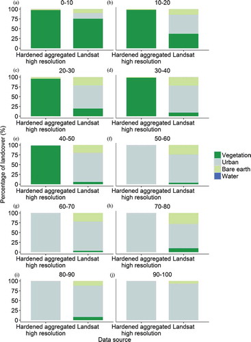
Figure 7. Comparison of percentage urban area aggregated to 30 m² from high-resolution data (a) and IVM ‘soft’ Landsat classification (b) highlighting the (overestimation) between the high (c) and moderate (d) spatial resolution estimates for the East Beechboro subset. The classified high spatial resolution data are shown in (e) with the moderate spatial resolution grid (30 m²) overlaid for context (e).

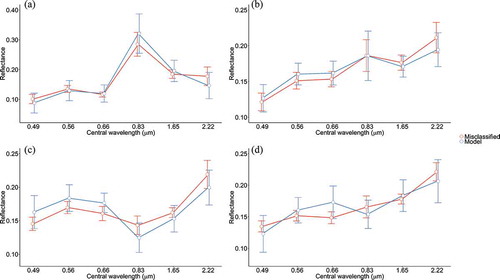
The results in Figure 6 suggest that the spectral data used to train the IVM classification (discussed in Section 4.2) contained spectrally ‘mixed’ pixels resulting in land-cover type misclassification. To investigate this, the spectral reflectance from Landsat pixels containing 20–30% urban cover for the Palmrya subset, which had the lowest overall agreement and which were identified as being mostly vegetated by the hardened high spatial resolution land-cover data set, is extracted and compared to the spectral reflectance profiles used to train the IVM classification algorithm. Figure 8 indicates that there are strong similarities between the average spectral reflectance profile used to train the IVM classification algorithm and the average spectral profile of the misclassified pixels. This suggests that the IVM classification algorithm is accurately representing the Landsat pixel spectral reflectance properties but that the training data used to develop the classification model contained a high proportion of mixed pixels.

Figure 8. Average spectral reflectance profile for misclassified pixels (red) from the Palmrya subset for pixels containing 20–30% urban cover compared to the average spectral reflectance profile of pixels used to train the IVM classification algorithm (blue). For (a) forest, (b) low urban reflectance, (c) high urban reflectance, and (d) bare earth. The error bars show the standard deviation.

Pure (i.e. homogeneous) pixels are conventionally selected to train classification models (e.g. Weng and Ruiliang 2013) but these are inherently difficult to identify in urban areas owing to the multitude of land covers within a Landsat pixel area. Using the high spatial resolution classification, the percentage of pure pixels, defined here as those containing between 90% and 100% of a single land-cover type, was identified (Table 4). It is evident that some regions contain a high percentage of pure pixels for a given land-cover type, such as vegetation in Keysbrook (92.05%), but that other land-cover types within a region typically have much lower percentages of pure pixels. Pure urban pixels are particularly limited in all subset regions. Whilst the CBD subset obtains a high percentage of pure urban pixels (28.77%), these are predominately urban areas with high spectral reflectance (e.g. concrete), differing from subsets with urban areas which have urban areas with both high and low spectral reflectance (e.g. East Beechboro; Figure 2).

Table 4. Percentage of ‘pure’ pixels (defined here as comprising 90–100% of given land cover within a Landsat pixel area) from the high-spatial resolution imagery.

Subset	Vegetation (%)	Urban (%)	Bare earth (%)	Water (%)
East Beechboro	53.93	0.15	0.34	0.03
CBD	8.98	28.77	0.35	0.00
Palmrya	5.80	2.13	0.00	0.01
Keysbrook	92.05	0.00	0.00	0.00

5.2. Comparison between Landsat and high spatial resolution impervious surface estimates

Landsat data have been widely applied to map impervious surface area in order to assess its effects on: urban growth dynamics (J. G. Masek, Lindsay, and Goward 2000), the UHI effect (Y. Hu et al. 2015), and surface run-off (Q. Weng 2001). Figure 6 indicates that the ‘hardened’ Landsat IVM classification overestimates urban land cover, particularly for pixels containing <50% urban area. The IVM classifier also provides a ‘soft’ land-cover data set that quantifies the subpixel land-cover proportions.

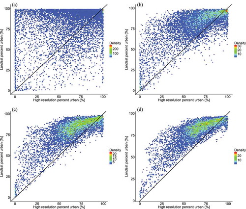
Here, we investigate the utility of the subpixel Landsat urban land-cover estimates by comparing them to those derived from the high spatial resolution land-cover data set (20 cm) which is used to provide the actual land-cover proportion within each 30 m² pixel area. Urban area estimates from each of the four subsets (Figure 1(a)) were spatially averaged over different size spatial windows (30 × 30, 90 × 90, 150 × 150, and 210 × 210 m) in order to account for any errors resulting from pixel heterogeneity, spatial mis-registration, residual atmospheric and BRDF effects, and phenological differences (Ju et al. 2012; Liang, Fang, and Chen 2001; Maiersperger et al. 2013; Ghimire, Rogan, and Miller 2010; Lu, Moran, and Hetrick 2011) that may increase the uncertainty in estimating land-cover proportions (Sexton et al. 2013; Lu, Moran, and Hetrick 2011). Comparison of impervious surface proportions at 30 m², for example the CBD subset (Figure 9), reiterates the overestimation of urban area at 30 m² spatial resolution, with a clustering of values towards the upper percentage boundaries associated with lower urban area estimates from the high spatial resolution classification. When neighbourhood averaging is applied, the agreement in urban area typically improves with increasing window size although the subset specific bias remains consistent (Table 5). It is also evident that urban area is still overestimated with decreasing urban subpixel proportion even when utilizing the subpixel IVM Landsat classification results.

Table 5. Comparison between high (20 cm²) and moderate (30 m²) spatial resolution subpixel impervious surface estimates considering differing kernel sizes over four subsets (Figure 1) within the PMR.

Subset	Kernel size (m)	R^2	Scatter	Bias	Root mean square error (RMSE)
East Beechboro	30 × 30	0.41*	26.65	18.68	32.54
	90 × 90	0.68*	16.95	18.66	25.21
	150 × 150	0.75*	14.11	18.71	23.44
	210 × 210	0.80*	12.52	18.74	22.54
CBD	30 × 30	0.26*	28.41	14.38	31.84
	90 × 90	0.53*	16.65	14.37	22.00
	150 × 150	0.61*	13.18	14.38	19.51
	210 × 210	0.66*	11.30	14.36	18.28
Palmrya	30 × 30	0.04*	26.65	34.54	43.62
	90 × 90	0.16*	13.56	34.61	37.17
	150 × 150	0.19*	10.15	34.64	36.10
	210 × 210	0.17*	8.45	34.67	35.69
Keysbrook	30 × 30	0.24*	11.85	2.51	12.11
	90 × 90	0.52*	7.47	2.51	7.88
	150 × 150	0.60*	5.89	2.50	6.40
	210 × 210	0.63*	4.98	2.50	5.57

*Statistically significant relationship (p < 0.05).

Figure 9. Relationship between the subpixel urban area percentage cover estimated from the IVM subpixel Landsat classification and the high spatial resolution orthophoto classification in the central business district (CBD) subset for (a) 30 × 30 m window, (b) 90 × 90 m window, (c) 150 × 150 m window, and (d) 210 × 210 m window.

5.3. Refining Landsat estimations using high spatial resolution data

Subpixel land-cover heterogeneity influences Landsat urban area overestimation which must be considered in order to reduce the bias and improve Landsat-derived urban area estimation (Herold et al. 2002; Lu, Moran, and Hetrick 2011; Varshney and Rajesh 2014; Schneider 2012). The complexity and diversity of urban areas identified here from high spatial resolution data, with biases ranging from −2.50% to −34.67%, highlights the inappropriateness of applying a single model to adjust the moderate spatial resolution urban area estimates in a metropolitan region (e.g. Lu, Moran, and Hetrick 2011). The Landsat subpixel urban areas estimates from all four subsets were stratified based on the Landsat subpixel derived urban area and calibrated against the percentage of urban area from the high spatial resolution classification within each moderate spatial resolution pixel area. Both data sets were averaged at the neighbourhood level using a 210 × 210 m window as this provided the best overall relationship (Table 5). Stratification of Landsat subpixel urban estimates into divisions of 10%, consistent with previous results, were selected to develop (using 50% of the data) and test (remaining 50% of the data) regression models to improve the data set agreement (Lu, Moran, and Hetrick 2011).

The applied spatially explicit models reduced the bias and root mean square error (RMSE) between the predicted (moderate spatial resolution) and observed (high spatial resolution) estimates (Table 6). It is evident from Table 6 that the adjustment made to the Landsat urban area estimates reduced the overestimation difference of urban area by between 34.38% and 80.67%, with the largest improvement found within Keysbrook. Whilst the corrected Landsat urban area estimates still overestimate the urban area compared to the high spatial resolution data set, the corrected moderate spatial resolution urban area reduces moderate resolution urban area over (under) estimation by on an average 55.08% in comparison to the high spatial resolution data set reducing the average overestimation from 11.86 km² per subset to just 0.09 km² (Table 6). In the case of this study area, this approach is appropriate for producing more accurate urban area statistics. Due to the frequently reported over and under estimation of land-cover estimates by moderate spatial resolution data, this approach can refine urban estimates for planning development policies that may inform decision-makers (Z. Zhu and Woodcock 2014; Schneider, Seto, and Webster 2005; Hepinstall-Cymerman, Coe, and Hutyra 2013). However, the derived correction values are not globally applicable since the spatial structure and makeup of urban and suburban areas varies regionally, nationally, and globally. Nevertheless, the methodology implemented here could be replicated to produce localized correction values from other sources of high-resolution imagery (e.g. digitization of Google Earth imagery) to calibrate urban area estimates from moderate spatial resolution data.

Table 6. Comparison between calibrated moderate (30 m²) and high (20 cm²) resolution subpixel impervious surface estimates with a kernel size of 210 m.

Subset	R^2	Bias	Root mean square error (RMSE)	High-resolution urban (km^2)	Uncorrected Landsat urban (km^2)	Uncorrected per cent difference to high resolution (%)	Corrected Landsat urban (km^2)	Corrected per cent difference to high resolution (%)
East Beechboro	0.84*	1.54	6.76	2.49	5.32	72.47	2.72	8.83
CBD	0.52*	−7.12	14.61	12.26	15.36	22.45	10.88	−11.93
Palmrya	0.12*	7.43	12.53	6.92	12.48	57.32	8.10	15.71
Keysbrook	0.62*	0.37	1.38	0.133	0.50	115.96	0.19	35.29

*Statistically significant relationship (p < 0.05).

6. Discussion

Refined urban estimates are vital in ensuring that suitable sustainable and strategic planning decisions are implemented (Bettencourt and West 2010; Wu and Murray 2003). The hybrid spatial resolution approach applied here to estimate urban area was necessary due to the difficulty in accurately estimating urban area using a traditional per-pixel classification method. This was due to a combination of the sensors moderate (30 m²) spatial resolution, land surface heterogeneity, and the selection of ‘mixed’ pixels for use in training the classification algorithm. The overall classification accuracy, determined using Google Earth imagery, was on an average 84.00%, which is similar to that found in other studies, albeit for different urban areas (e.g. Gislason, Benediktsson, and Sveinsson 2006; Bagan and Yamagata 2014; Sundarakumar et al. 2012; Luo et al. 2014).

Closer examination of the moderate spatial resolution classification results using a higher resolution data set indicates that when urban land cover within a 30 m² area decreases to 40–50% (based on high spatial resolution classification), the Landsat classification accuracy decreased from 85.40% to between 1.99% and 6.21%. This resulted from the Landsat classification overestimating urban area in comparison to high spatial resolution data (Figure 5) which more correctly identified these pixels as containing a greater per-pixel proportion of vegetation. Pixels containing 40–50% urban cover contained on an average 54.50% vegetation cover excluding Keysbrook. The dominance of vegetation and urban land covers in the regional subset, when ascribed to a 30 m² pixel area based on the majority land cover, results in a rapid change in classification accuracy. Strong spectral similarities between training data and misclassified pixels (Figure 8) suggest that the spectral reflectance observations used to train the classification algorithm contained spectrally mixed pixels. The average percentage urban area within a moderate spatial resolution pixel area derived from the high-resolution data was 16.56%, 65.66%, 42.21%, and 0.90% for East Beechboro, CBD, Palmyra, and Keysbrook, respectively. The percentage of ‘pure’ pixels, defined as those containing over 90% urban land cover, was 28.77% for the CBD but <2.50% for the suburban regional subsets. This highlights the difficulty in selecting pure pixels at moderate spatial resolution and in accurately disentangling mixed spectral reflectance’s without the aid of high spatial resolution data. Overestimation of urban extent was most prominent in Keysbrook, where vegetation dominates the subset (97.36%, Table 1). In this instance, Landsat-derived urban area corresponded to 0.28 km² compared to 0.08 km² from high spatial resolution classification, a difference of only 0.20 km² but which equates to 251.74%. In terms of total area difference, the East Beechboro and the CBD Landsat subsets were found to contain 1.75 and 1.70 km² more urbanized area, whilst Palmyra data overestimated urban area by 2.79 km² compared to the high spatial resolution equivalent due to its suburban nature and associated pixel heterogeneity (Figure 4).

Spatially averaging the Landsat and orthophoto land-cover classifications, to account for potential errors in the data sets (Ghimire, Rogan, and Miller 2010), improved their relationship although Landsat still overestimated urban area with differing bias per subset. Over (under) estimation of urban land from Landsat estimations could result in an under (over) prediction on further environmental variables (e.g. UHI) or policy applications. Multiple studies have used classified per-pixel moderate spatial resolution data to influence policy changes through monitoring urban growth (e.g. Schneider, Seto, and Webster 2005; Hepinstall-Cymerman, Coe, and Hutyra 2013). However, per-pixel methodologies fail to address the issue of mixed pixels, which, as shown here, can result in overestimation of urban area (average: 126.25%, equivalent to 57.58 km² within the PMR) (Lu, Moran, and Hetrick 2011). Subpixel methods attempt to remedy this issue but have been found to inaccurately separate impervious land cover from other land-cover types resulting in poor representation of impervious surface area (Lu, Moran, and Hetrick 2011). Consequently, overestimation of urban area may have resulted in suboptimal policies that fail to maximize resource and amenity efficiency (Turner, Lambin, and Reenberg 2010; Downs 2005).

Calibrating Landsat urban estimates using high spatial resolution data reduces the bias, RMSE, and improves urban area estimation. However, the range of bias values across subsets of differing urban land-cover characteristic highlights the inappropriateness of a single regression model due to pixel heterogeneity influencing overestimation (Lu, Moran, and Hetrick 2011). Spatially explicit models, as presented here, permit varying moderate spatial resolution refinement by considering the influence of surface heterogeneity. Whilst the limited availability of low-cost high spatial resolution data can preclude analysis of this type, subset digitization of Google Earth or unmanned aerial vehicle (UAV) imagery may provide a suitable alternative for calibrating Landsat data for improved urban area estimates. Enhanced estimates of urban area would facilitate planning policies that avoid potential environmental and socio-economic consequences of urban development than can result from policies based on over (or under) predicted urban area (ARUP, and The Rockefeller Foundation 2015). For example, classified Landsat data were used to identify spatial clustering, peri urban development, and specialization of land-use in Chengdu, Sichuan province, not considered by China’s original 1990 Go West policy, aimed at economically boosting the West of the country. Results were used to reform policy and remediate issues of urban management including service, infrastructure, and resource deficiencies (Schneider, Seto, and Webster 2005). However, traditional Landsat classification may over (or under) estimate urban area and result in ineffective planning, environmental, and policy decisions (Miller and Small 2003; Pravitasari et al. 2015). Therefore, classified subpixel data alongside high spatial resolution imagery (e.g. UAV, Google Earth, high spatial resolution aerial or satellite imagery) as presented here can refine urban estimates facilitating improved decision-making whilst maximizing often limited financial resources. This is especially important in developing countries in regards to directing urban development and resources based on factors including poverty, environmental hazards (e.g. flooding), and current amenity centres (Marfai, Sekaranom, and Ward 2014; Suryahadi and Sumarto 2003).

7. Conclusion

Landsat imagery from 2007 was used to map the urban extent within the PMR using an IVM classifier that provides both a per-pixel and a subpixel classified data sets. The 2007 Landsat classification overall average accuracy was 84.00% with associated kappa coefficient of 0.78. Comparison between the Landsat per-pixel urban area and urban area estimates obtained from a high spatial resolution (20 cm) orthophoto-derived classification indicates that the moderate spatial resolution classification overestimates urban extent by 126.25% on an average, which is equivalent to 57.58 km² in the study area. Similarly, when the high spatial resolution urban area estimates are compared to those derived using a subpixel Landsat classification, the latter still overestimates urban extent by 120.25%.

Accurately quantifying urban expansion within the PMR due to the large population growth over the last decade is important in order to make the efficient use of current resources and to avoid additional amenity, environmental and health expenditure that can impact sprawling cities. Landsat data provide the longest time series of medium spatial resolution imagery to map and monitor urban area. However, the reported over and underestimation inhibits accurate quantification of urbanized land cover which increases uncertainty within global climate models, environmental studies, and targeted urban planning policy. Neighbourhood averaging, to account for potential errors in the data sets, improved the agreement between the two data sets but Landsat subpixel overestimation still remained. The broad differences in bias between the difference subsets indicate that a single regression model is inappropriate to heterogeneous urban land-cover estimates. Therefore, the moderate spatial resolution urban area estimates were corrected using spatially explicit regression models which, on an average, across the four subsets reduced the bias and RMSE by 17.02 and 6.65 km² respectively, whilst reducing moderate resolution urban area over (under) estimation by 55.08%

Current and future EO satellites that provide complimentary data with enhanced spatial, spectral, and temporal resolution, such as Sentinel-2, may further reduce over or underestimation of urban area experienced by moderate spatial resolution sensors such as Landsat. Similarly, high spatial resolution satellite sensors, such as Worldview-3, are able to remediate discrepancies by capturing the fine spatial detail of urban environments but their cost and small swath limit their widespread application. This might change with companies, such as Planet, which are launching large numbers of small microsatellites that provide high spatial resolution data more frequently. Accurate urban land-cover and land-use mapping is essential in understanding the impact of urban expansion on, for example, social–ecological systems and human health and will improve future sustainable planning of our cities.

Geolocation Information

This research was conducted over the Perth Metropolitan Region, Western Australia, Australia, 31.9505°S, 115.8605°E.

Acknowledgements

This work was supported by the Economic and Social Research Council: [Grant Number ES/J500161/1]. We would like to thank the World University Network (WUN) for facilitating institutional visits, the University of Western Australia for supplying high-resolution orthophotos of the Perth Metropolitan Region and the United States Geological Survey (USGS) for providing Landsat surface reflectance imagery.

Disclosure statement

No potential conflict of interest was reported by the authors.

Supplemental data

Supplemental data for this article can be accessed here.

Additional information

Funding

This work was supported by the Economic and Social Research Council: [Grant Number ES/J500161/1] .

References

- ABS. 2015. Australian National Accounts 1988-2015. Australian Bureau of Statistics. Belconnen, ACT, Australia.
- Aguilar, M. A., R. Vicente, F. J. Aguilar, A. Fernández, and M. M. Saldaña. 2012. “Optimizing Object-Based Classification in Urban Environments Using Very High Resolution Geoeye-1 Imagery.” ISPRS Annals of the Photogrammetry, Remote Sensing and Spatial Information Sciences 1–7: 99–104. doi:10.5194/isprsannals-I-7-99-2012.
- Akbari, H., S. Rose, and H. Taha. 2003. “Analyzing the Land Cover of an Urban Environment Using High-Resolution Orthophotos.” Landscape and Urban Planning 63 (1): 1–14. doi:10.1016/S0169-2046(02)00165-2.
- ARUP, and The Rockefeller Foundation. 2015. City Resilience Framework—100 Resilient Cities. New York, NY, USA: Rockefeller Foundation.
- Bagan, H., and Y. Yamagata. 2014. “Land-Cover Change Analysis in 50 Global Cities by Using a Combination of Landsat Data and Analysis of Grid Cells.” Environmental Research Letters 9(6). IOP Publishing: 64015. doi:10.1088/1748-9326/9/6/064015.
- Bettencourt, L., and G. West. 2010. “A Unified Theory of Urban Living.” Nature 467 (913): 9–10. doi:10.1038/467912a.
- Braun, A. C., U. Weidner, and S. Hinz. 2012. “Classification in High-Dimensional Feature Spaces-Assessment Using SVM, IVM and RVM with Focus on Simulated EnMAP Data.” IEEE Journal of Selected Topics in Applied Earth Observations and Remote Sensing 5 (2): 436–443. doi:10.1109/JSTARS.2012.2190266.
- Caccetta, P., S. Collings, A. Devereux, K. Hingee, D. Mcfarlane, A. Traylen, and W. Xiaoliang. 2012. Urban Monitor : Enabling Effective Monitoring and Management of Urban and Coastal Environments Using Digital Aerial Photography Final Report – Transformation of Aerial Photography into Digital Raster Information Products. Australia: CSIRO.
- Cai, Y., H. Zhang, P. Zheng, and W. Pan. 2016. “Quantifying the Impact of Land use/Land Cover Changes on the Urban Heat Island: A Case Study of the Natural Wetlands Distribution Area of Fuzhou City, China.” Wetlands. doi:10.1007/s13157-016-0738-7.
- Chen, T., R. A. M. De Jeu, Y. Y. Liu, G. R. Van Der Werf, and A. J. Dolman. 2014. “Using Satellite Based Soil Moisture to Quantify the Water Driven Variability in NDVI: A Case Study over Mainland Australia.” Remote Sensing of Environment 140: 330–338. doi:10.1016/j.rse.2013.08.022.
- Collings, S., P. Caccetta, and N. Campbell. 2011. “Empirical Models for Radiometric Calibration of Digital Aerial Frame Mosaics.” IEEE Transactions on Geoscience and Remote Sensing 49 (7): 2573–2588. doi:10.1109/TGRS.2011.2108301.
- Congalton, R. G. 2001. “Accuracy Assessment and Validation of Remotely Sensed and Other Spatial Information.” International Journal of Wildland Fire 10: 321–328. doi:10.1071/WF01031.
- Cunningham, S., J. Rogan, D. Martin, V. DeLauer, S. McCauley, and A. Shatz. 2015. “Mapping Land Development through Periods of Economic Bubble and Bust in Massachusetts Using Landsat Time Series Data.” GIScience & Remote Sensing 1603: 2016. doi:10.1080/15481603.2015.1045277.
- Department for Communities and Local Government. 2015. English Housing Survey: Housing Stock Report, 2014-2015. London, UK: English Housing Survey. doi:10.1017/CBO9781107415324.004.
- Dhakal, S. P. 2014. “Glimpses of Sustainability in Perth, Western Australia : Capturing and Communicating the Adaptive Capacity of an Activist Group.” Consilience: the Jounral of Sustainable Development 11 (1): 167–182.
- Dorais, A., and J. Cardille. 2011. “Strategies for Incorporating High-Resolution Google Earth Databases to Guide and Validate Classifications: Understanding Deforestation in Borneo.” Remote Sensing 3 (6): 1157–1176. doi:10.3390/rs3061157.
- Downs, A. 2005. “Smart Growth: Why We Discuss It More than We Do It.” Journal of the American Planning Association 71 (4): 367–378. doi:10.1080/01944360508976707.
- Feyisa, G. L., G. Henrik Meilby, D. Jenerette, and S. Pauliet. 2016. “Locally Optimized Separability Enhancement Indices for Urban Land Cover Mapping: Exploring Thermal Environmental Consequences of Rapid Urbanization in Addis Ababa, Ethiopia.” Remote Sensing of Environment 175: 14–31. doi:10.1016/j.rse.2015.12.026.
- Foody, G. M., and A. Mathur. 2006. “The Use of Small Training Sets Containing Mixed Pixels for Accurate Hard Image Classification: Training on Mixed Spectral Responses for Classification by a SVM.” Remote Sensing of Environment 103 (2): 179–189. doi:10.1016/j.rse.2006.04.001.
- Friedl, M. A., D. K. McIver, J. C. F. Hodges, X. Y. Zhang, D. Muchoney, A. H. Strahler, C. E. Woodcock, et al. 2002. “Global Land Cover Mapping from MODIS: Algorithms and Early Results.” Remote Sensing of Environment 83 (1–2): 287–302. doi:10.1016/S0034-4257(02)00078-0.
- Ghimire, B., J. Rogan, and J. Miller. 2010. “Contextual Land-Cover Classification: Incorporating Spatial Dependence in Land-Cover Classification Models Using Random Forests and the Getis Statistic.” Remote Sensing Letters 1 (1): 45–54. doi:10.1080/01431160903252327.
- Gislason, P. O., J. A. Benediktsson, and J. R. Sveinsson. 2006. “Random Forests for Land Cover Classification.” Pattern Recognition Letters 27 (4): 294–300. doi:10.1016/j.patrec.2005.08.011.
- Hansen, M. C., and T. R. Loveland. 2012. “A Review of Large Area Monitoring of Land Cover Change Using Landsat Data.” Remote Sensing of Environment 122: 66–74. doi:10.1016/j.rse.2011.08.024.
- Hepinstall-Cymerman, J., S. Coe, and L. R. Hutyra. 2013. “Urban Growth Patterns and Growth Management Boundaries in the Central Puget Sound, Washington, 1986-2007.” Urban Ecosystems 16 (1): 109–129. doi:10.1007/s11252-011-0206-3.
- Herold, M., M. Gardner, B. Hadley, and D. Roberts. 2002. “The Spectral Dimension in Urban Land Cover Mapping from High-Resolution Optical Remote Sensing Data.” Symposium A Quarterly Journal In Modern Foreign Literatures 6: 1–8. doi:10.1109/TGRS.2003.815238.
- Howard, L. 1988. The Climate of London. London, UK: Cambridge University Press.
- Hu, L., and N. A. Brunsell. 2015. “A New Perspective to Assess the Urban Heat Island through Remotely Sensed Atmospheric Profiles.” Remote Sensing of Environment 158: 393–406. doi:10.1016/j.rse.2014.10.022.
- Hu, X., and Q. Weng. 2009. “Estimating Impervious Surfaces from Medium Spatial Resolution Imagery Using the Self-Organizing Map and Multi-Layer Perceptron Neural Networks.” Remote Sensing of Environment 113 (10): 2089–2102. doi:10.1016/j.rse.2009.05.014.
- Hu, Y., G. Jia, M. Hou, X. Zhang, F. Zheng, and Y. Liu. 2015. “The Cumulative Effects of Urban Expansion on Land Surface Temperatures in Metropolitan Jingjintang, China Yonghong.” Journal of Geophysical RESEARCH: Atmospheres RESEARCH 9932–9943. doi:10.1002/2014JD022994.Received.
- Huang, C., L. S. Davis, and J. R. G. Townshend. 2002. “An Assessment of Support Vector Machines for Land Cover Classification.” International Journal of Remote Sensing 23 (4): 725–749. doi:10.1080/01431160110040323.
- Imhoff, M. L., W. T. Lawrence, D. C. Stutzer, and C. D. Elvidge. 1997. “A Technique for Using Composite DMSP/OLS ‘City Lights’ Satellite Data to Map Urban Area.” Remote Sensing of Environment 61 (3): 361–370. doi:10.1016/S0034-4257(97)00046-1.
- Ju, J., D. P. Roy, E. Vermote, J. Masek, and V. Kovalskyy. 2012. “Continental-Scale Validation of MODIS-Based and LEDAPS Landsat ETM+ Atmospheric Correction Methods.” Remote Sensing of Environment 122: 175–184. doi:10.1016/j.rse.2011.12.025.
- Kalnay, E., and M. Cai. 2003. “Impact of Urbanization and Land-Use Change on Climate.” Nature 423: 528–531. doi:10.1038/nature01649.1.
- Kelly, J. F., B. Weidmann, and M. Walsh. 2011. The Housing We’d Choose. Grattan Institute. Melbourne, Australia: Grattan Institute.
- Kennewell, C., and B. J. Shaw. 2008. “Perth, Western Australia.” Cities 25 (4): 243–255. doi:10.1016/j.cities.2008.01.002.
- Kotsiantis, S. B., I. D. Zaharakis, and P. E. Pintelas. 2006. “Machine Learning: A Review of Classification and Combining Techniques.” Artificial Intelligence Review 26 (3): 159–190. doi:10.1007/s10462-007-9052-3.
- Li, C., J. Wang, L. Wang, H. Luanyun, and P. Gong. 2014. “Comparison of Classification Algorithms and Training Sample Sizes in Urban Land Classification with Landsat Thematic Mapper Imagery.” Remote Sensing 6 (2): 964–983. doi:10.3390/rs6020964.
- Liang, S., H. Fang, and M. Chen. 2001. “Atmospheric Correction of Landsat ETM+ Land Surface Imagery. I.\nMethods.” IEEE Transactions on Geoscience and Remote Sensing 39 (11): 2490–2498. doi:10.1109/36.964986.
- Lu, D., L. Guiying, W. Kuang, and E. Moran. 2014. “Methods to Extract Impervious Surface Areas from Satellite Images.” International Journal of Digital Earth 7 (2015): 93–112. doi:10.1080/17538947.2013.866173.
- Lu, D., E. Moran, and S. Hetrick. 2011. “Detection of Impervious Surface Change with Multitemporal Landsat Images in an Urban-Rural Frontier.” ISPRS Journal of Photogrammetry and Remote Sensing : Official Publication of the International Society for Photogrammetry and Remote Sensing (ISPRS) 66 (3): 298–306. doi:10.1016/j.isprsjprs.2010.10.010.
- Lu, D., and Q. Weng. 2006. “Use of Impervious Surface in Urban Land-Use Classification.” Remote Sensing of Environment 102 (1–2): 146–160. doi:10.1016/j.rse.2006.02.010.
- Luo, J., D. Peijun, S. Alim, X. Xie, and Z. Xue. 2014. “Annual Landsat Analysis of Urban Growth of Nanjing City from 1980 to 2013.” 2014 Third International Workshop on Earth Observation and Remote Sensing Applications (EORSA) 357–361. doi:10.1109/EORSA.2014.6927912.
- MacLachlan, A., E. Biggs, G. Roberts, and B. Boruff. 2017a. “Urban Growth Dynamics in Perth, Western Australia: Using Applied Remote Sensing for Sustainable Future Planning.” Land 6 (1): 9. doi:10.3390/land6010009.
- MacLachlan, A., E. Biggs, G. Roberts, and B. Boruff. 2017b. Classified Earth Observation Data between 1990 and 2015 for the Perth Metropolitan Region, Western Australia Using the Import Vector Machine Algorithm. PANGAEA. doi:10.1594/PANGAEA.871017.
- Maiersperger, T. K., P. L. Scaramuzza, L. Leigh, S. Shrestha, K. P. Gallo, C. B. Jenkerson, and J. L. Dwyer. 2013. “Characterizing LEDAPS Surface Reflectance Products by Comparisons with AERONET, Field Spectrometer, and MODIS Data.” Remote Sensing of Environment 136: 1–13. doi:10.1016/j.rse.2013.04.007.
- Marfai, M. A., A. B. Sekaranom, and P. Ward. 2014. “Community Responses and Adaptation Strategies toward Flood Hazard in Jakarta, Indonesia.” Natural Hazards 75 (2): 1127–1144. doi:10.1007/s11069-014-1365-3.
- Masek, J. G., E. F. Vermote, N. E. Saleous, R. Wolfe, F. G. Hall, K. F. Huemmrich, F. Gao, J. Kutler, and T.-K. Lim. 2006. “A Landsat Surface Reflectance Dataset.” IEEE Geoscience and Remote Sensing Letters 3 (1): 68–72. doi:10.1109/LGRS.2005.857030.
- Masek, J. G., F. E. Lindsay, and S. N. Goward. 2000. “Dynamics of Urban Growth in the Washington DC Metropolitan Area, 1973-1996, from Landsat Observations.” International Journal of Remote Sensing 21 (18): 3473–3486. doi:10.1080/014311600750037507.
- Miller, R. B., and C. Small. 2003. “Cities from Space: Potential Applications of Remote Sensing in Urban Environmental Research and Policy.” Environmental Science and Policy 6 (2): 129–137. doi:10.1016/S1462-9011(03)00002-9.
- Mountrakis, G., I. Jungho, and C. Ogole. 2011. “Support Vector Machines in Remote Sensing: A Review.” ISPRS Journal of Photogrammetry and Remote Sensing 66 (3): 247–259. doi:10.1016/j.isprsjprs.2010.11.001.
- Myint, S. W., P. Gober, A. Brazel, S. Grossman-Clarke, and Q. Weng. 2011. “Per-Pixel Vs. Object-Based Classification of Urban Land Cover Extraction Using High Spatial Resolution Imagery.” Remote Sensing of Environment 115 (5): 1145–1161. doi:10.1016/j.rse.2010.12.017.
- Pal, M., and P. M. Mather. 2003. “An Assessment of the Effectiveness of Decision Tree Methods for Land Cover Classification.” Remote Sensing of Environment 86 (4): 554–565. doi:10.1016/S0034-4257(03)00132-9.
- Pan, J., M. Wang, D. Li, and J. Li. 2009. “Automatic Generation of Seamline Network Using Area Voronoi Diagrams with Overlap.” IEEE Transactions on Geoscience and Remote Sensing 47 (6): 1737–1744. doi:10.1109/TGRS.2008.2009880.
- Powell, R., and D. Roberts. 2008. “Characterizing Variability of the Urban Physical Environment for a Suite of Cities in Rondônia, Brazil.” Earth Interactions 12 (13): 1–32. doi:10.1175/2008EI246.1.
- Powell, R., and D. Roberts. 2010. “Characterizing Urban Land-Cover Change in Rondônia, Brazil: 1985 to 2000.” Journal of Latin American Geography 9 (3): 183–211. doi:10.1353/lag.2010.0028.
- Powell, R., D. Roberts, P. Dennison, and L. Hess. 2007. “Sub-Pixel Mapping of Urban Land Cover Using Multiple Endmember Spectral Mixture Analysis: Manaus, Brazil.” Remote Sensing of Environment 106 (2): 253–267. doi:10.1016/j.rse.2006.09.005.
- Poznanska, A., S. Bayer, and T. Bucher. 2013. “Derivation of Urban Objects and Their Attributes for Large-Scale Urban Areas Based on Very High Resolution UltraCam True Orthophotos and nDSM – a Case Study Berlin, Germany.” Proceedings of the SPIE 13. doi:10.1117/12.2030000.
- Pravitasari, A. E., I. Saizen, N. Tsutsumida, E. Rustiadi, and D. O. Pribadi. 2015. “Local Spatially Dependent Driving Forces of Urban Expansion in an Emerging Asian Megacity: The Case of Greater Jakarta (Jabodetabek).” Journal of Sustainable Development 8 (1): 108–120. doi:10.5539/jsd.v8n1p108.
- Ridd, M. K. 1995. “Exploring A V-I-S Model for Urban Ecosystem through Remote Sensing: A Comparative Ananomy for Cities.” International Journal of Remote Sensing. doi:10.1080/01431169508954549.
- Roscher, R., W. Förstner, and B. Waske. 2012. “I 2VM: Incremental Import Vector Machines.” Image and Vision Computing 30: 263–278. doi:10.1016/j.imavis.2012.04.004.
- Roscher, R., B. Waske, and W. Forstner. 2010. “Kernel Discriminative Random Fields for Land Cover Classification.” APR Workshop on Pattern Recognition in Remote Sensing. doi:10.1109/PRRS.2010.5742801.
- Schneider, A. 2012. “Monitoring Land Cover Change in Urban and Peri-Urban Areas Using Dense Time Stacks of Landsat Satellite Data and a Data Mining Approach.” Remote Sensing of Environment 124: 689–704. doi:10.1016/j.rse.2012.06.006.
- Schneider, A., M. Friedl, and D. Potere. 2010. “Mapping Global Urban Areas Using MODIS 500-M Data: New Methods and Datasets Based on ‘Urban Ecoregions.’.” Remote Sensing of Environment 114 (8): 1733–1746. doi:10.1016/j.rse.2010.03.003.
- Schneider, A., M. A. Friedl, and D. Potere. 2009. “A New Map of Global Urban Extent from MODIS Satellite Data.” Environmental Research Letters 4 (4): 44003. doi:10.1088/1748-9326/4/4/044003.
- Schneider, A., and C. M. Mertes. 2014. “Expansion and Growth in Chinese Cities, 1978–2010.” Environmental Research Letters 9 (2): 24008. doi:10.1088/1748-9326/9/2/024008.
- Schneider, A., K. Seto, and D. Webster. 2005. “Urban Growth in Chengdu, Western China: Application of Remote Sensing to Assess Planning and Policy Outcomes.” Environment and Planning B: Planning and Design 32 (3): 323–345. doi:10.1068/b31142.
- Sexton, J. O., X.-P. Song, C. Huang, C. Saurabh, M. E. Baker, and J. R. Townshend. 2013. “Urban Growth of the Washington, D.C.–Baltimore, MD Metropolitan Region from 1984 to 2010 by Annual, Landsat-Based Estimates of Impervious Cover.” Remote Sensing of Environment 129: 42–53. doi:10.1016/j.rse.2012.10.025.
- Sharifi, E., and S. Lehmann. 2014. “Comparative Analysis of Surface Urban Heat Island Effect in Central Sydney.” Journal of Sustainable Development 7 (3): 23–34. doi:10.5539/jsd.v7n3p23.
- Song, X.-P., J. O. Sexton, C. Huang, S. Channan, and J. R. Townshend. 2016. “Characterizing the Magnitude, Timing and Duration of Urban Growth from Time Series of Landsat-Based Estimates of Impervious Cover.” Remote Sensing of Environment 175: 1–13. doi:10.1016/j.rse.2015.12.027.
- Sun, G., X. Chen, X. Jia, Y. Yao, and Z. Wang. 2015. “Combinational Build-Up Index (CBI) for Effective Impervious Surface Mapping in Urban Areas.” IEEE Journal of Selected Topics in Applied Earth Observations and Remote Sensing 1–12. doi:10.1109/JSTARS.2015.2478914.
- Sundarakumar, K., M. Harika, S. K. Aspiya Begum, S. Yamini, and K. Balakrishna. 2012. “Land Use And Land Cover Change Detection And Urban Sprawl Analysis Of Vijayawada City Using Multitemporal Landsat.” International Journal of Engineering Science and Technology 4 (1): 170–178.
- Suryahadi, A., and S. Sumarto. 2003. “Poverty and Vulnerability in Indonesia before and after the Economic Crisis.” Asian Economic Journal 17 (1): 45–64. doi:10.1111/1351-3958.00161.
- Turner, B., E. Lambin, and A. Reenberg. 2010. “The Emergence of Land Change Science for Global Environmental Change and Sustainability.” PNAS 103 (128): 13070–13075. doi:10.1073/pnas.0704119104.
- U.S. Department of Commerce. 2013. 2013 Housing Profile: United States. U.S. Department of Housing and Uban Development. Washington, USA: United States Census Bureau.
- United Nations, Department of Economic and Social Affairs, Population Division. 2014. World Urbanization Prospects: The 2014 Revision, Highlights (ST/ESA/SER.A/352). New York, NY, USA. doi:10.4054/DemRes.2005.12.9.
- Varshney, A., and E. Rajesh. 2014. “A Comparative Study of Built-Up Index Approaches for Automated Extraction of Built-Up Regions from Remote Sensing Data.” Journal of the Indian Society of Remote Sensing 42: 1–5. doi:10.1007/s12524-013-0333-9.
- Vermote, E., D. Tanre, J. L. Deuze, M. Herman, and J. J. Morcrette. 1997. Second Simulation of the Satellite Signal in the Solar Spectrum (6S). 6S User Guide Version 2. Appendix III: Description of the Subroutines. Maryland, USA: NASA-Goddard Space Flight Center.
- Wang, L., D. Liu, Q. Wang, and Y. Wang. 2013. “Spectral Unmixing Model Based on Least Squares Support Vector Machine with Unmixing Residue Constraints.” Ieee Geoscience and Remote Sensing Letters 10 (6): 1592–1596. 10.1109/LGRS.2013.2262371.
- Wanner, W., X. Li, and A. H. Strahler. 1995. “On the Derivation of Kernels for Kernel-Driven Models of Bidirectional Reflectance.” Journal of Geophysical Research 100 (D10): 21077. doi:10.1029/95JD02371.
- Watanachaturaporn, P., M. K. Arora, and P. K. Varshney. 2008. “Multisource Classification Using Support Vector Machines: An Empirical Comparison with Decision Tree and Neural Network Classifiers.” Photogrammetric Engineering and Remote Sensing 74 (2): 239–246. doi:10.14358/PERS.74.2.239.
- Weng, F., and P. Ruiliang. 2013. “Mapping and Assessing of Urban Impervious Areas Using Multiple Endmember Spectral Mixture Analysis: A Case Study in the City of Tampa, Florida.” Geocarto International 28 (7): 594–615. doi:10.1080/10106049.2013.764355.
- Weng, Q. 2001. “Modeling Urban Growth Effects on Surface Runoff with the Integration of Remote Sensing and GIS.” Environmental Management 28 (6): 737–748. doi:10.1007/s002670010258.
- Western Australian Planning Commission. 2013a. The Housing We’d Choose: A Study for Perth and Peel. the Government of Western Australia Department of Housing and Department of Planning. Perth,WA, Australia: Western Australian Planning Commission.
- Western Australian Planning Commission. 2013b. The Housing We’d Choose: A Study for Perth and Peel Summary Report. Perth,WA, Australia: Western Australian Planning Commission.
- Western Australian Planning Commission. 2015. Perth and Peel @ 3.5 Million. the Government of Western Australia Department of Planning. Perth,WA, Australia: Western Australian Planning Commission.
- Wilson, E. H., J. D. Hurd, D. L. Civco, M. P. Prisloe, and C. Arnold. 2003. “Development of a Geospatial Model to Quantify, Describe and Map Urban Growth.” Remote Sensing of Environment 86 (3): 275–285. doi:10.1016/S0034-4257(03)00074-9.
- Wu, C., and A. T. Murray. 2003. “Estimating Impervious Surface Distribution by Spectral Mixture Analysis.” Remote Sensing of Environment 84: 493–505. doi:10.1016/S0034-4257(02)00136-0.
- Xie, Q., and Z. Zhou. 2015. “Impact Of Urbanization On Urban Heat Island Effect Based On TM Imagery In Wuhan, China.” Environmental Engineering and Management Journal 14 (3): 647–655.
- Yuan, F., K. E. Sawaya, B. C. Loeffelholz, and M. E. Bauer. 2005. “Land Cover Classification and Change Analysis of the Twin Cities (Minnesota) Metropolitan Area by Multitemporal Landsat Remote Sensing.” Remote Sensing of Environment 98 (2): 317–328. doi:10.1016/j.rse.2005.08.006.
- Zhu, J., and T. Hastie. 2005. “Kernel Logistic Regression and the Import Vector Machine.” Journal of Computational and Graphical Statistics 14 (2015): 185–205. doi:10.1198/106186005X25619.
- Zhu, Z., and C. E. Woodcock. 2014. “Continuous Change Detection and Classification of Land Cover Using All Available Landsat Data.” Remote Sensing of Environment 144: 152–171. doi:10.1016/j.rse.2014.01.011.