A seasonal climatology of UV reflectivity for southern South America

ABSTRACT

A seasonal climatology for the Lambertian equivalent reflectivity (LER) in ultraviolet (UV) for southern South America is introduced. The study region was limited by 10° and 60°S and by 100° and 30°W; the data set spanned the period 1978–2015. Features of the seasonal means and of the quarterly (Q) and the interannual (IA) variabilities for each season were ascribed to atmospheric and oceanic processes of local, regional, or global origin which lead to the formation or maintenance of clouds. Shifts in the Q and IA time series were detected, most notably in the early 1990s. Linear trends were also estimated. The largest positive and negative trends in the Q time series were found along the Peruvian Andes (PA) (3.20 reflectivity units [RU] decade⁻¹) and east of the Chapada Diamantina (CD) and the Serra do Espinhaço (SE) in Brazil (−1.40 RU decade⁻¹), respectively. The largest positive and negative trends in the IA time series were found in PA (6 RU decade⁻¹, summer) and east of CD and SE (−2.50 RU decade⁻¹, spring), respectively. The linkages between UV LER and regional or global circulation indices were also studied. The largest relationships were found with the Dipole Mode Index on a Q basis and with the Southern Oscillation Index on an IA basis in winter.

1. Introduction

The Earth’s climate system is a consequence of complex interplays between its subcomponents (Levitus et al. 2001; Rial et al. 2004; Seinfeld et al. 2004). Its state is mainly driven by the balance between the heating created by the incoming solar radiation, mainly consisting of near ultraviolet (UV), visible, and near-infrared wavelengths, and the cooling by the infrared (or terrestrial) outgoing longwave radiation (OLR) (Ramanathan 1988; Charlson et al. 2007; Herman et al. 2013). Changes in this energy balance induce climate perturbations having the most notable impact in temperature (Kaufman and Fraser 1997; Seinfeld and Pandis 2016). The Intergovernmental Panel on Climate Change’s (IPCC’s) Fifth Assessment Report stressed that ‘each of the last three decades has been successively warmer at the Earth’s surface than any preceding decade since 1850’ (IPCC 2013). This warming may at least partly rely upon the contribution of aerosols and clouds to the Earth’s radiation budget (Charlson et al. 1992; Hess, Koepke, and Schult 1998); yet, there exist large uncertainties over both specific role of aerosols and clouds in climate change processes and interactions between these constituents of the atmosphere (Boucher et al. 2013).

Atmospheric aerosols are a complex chemical mixture of airborne solid and/or liquid particles. Local variations in the properties of both natural and anthropogenic aerosols are considered a ‘climate forcing’ that modulates the Earth’s radiation balance (Charlson et al. 1992; Hansen et al. 1997). This climate forcing relies upon the particles’ size, chemical composition, shape, and concentration, among other parameters (Charlson et al. 1992; Ghan et al. 2012). The effects aerosols have in the Earth’s radiation budget can be classified in direct, indirect, and semi-direct. The direct effect involves scattering and absorption of solar radiation, and scattering, absorption, and emission of terrestrial radiation, disregarding in all cases the effects on clouds (Charlson et al. 1992; Lohmann and Feichter 2005; Ghan et al. 2012). As to the indirect effect, they act as cloud condensation nuclei and ice nuclei and ultimately affect the emissivity and the reflectivity of clouds (Ghan et al. 2012). The semi-direct effect is a mixture of both previous effects: absorption heats the air and may lead to evaporation, therefore changing the clouds’ properties (Lohmann and Feichter 2005). Both direct and indirect effects tend to reduce the amount of solar radiation that reaches the Earth’s surface, whereas there is a heating in the atmospheric column due to the semi-direct effect. In addition to the impacts on temperature, aerosols also interfere with precipitation (Ramanathan et al. 2001). They could also influence the hydrological cycle through a reduction in evaporation to the extent that it can spin down the water cycle (Liepert et al. 2004).

On the other hand, the study of clouds is crucial for the understanding of the energy balance and for a proper assessment of climate change. The Earth’s cloud cover consists of a palette of different cloud types, ranging from low-level boundary layer clouds (fog) to high-level deep convective clouds (anvils) spanning most of the troposphere. Nearly 70% of the Earth’s surface is covered with clouds (IPCC 2013). They play an important role as regulators of the Earth’s radiation budget. Simply stated, clouds reflect a large fraction of the incoming solar radiation back to space and absorb terrestrial radiation and reemit it at the temperature of their tops (Ramanathan et al. 1989). The effects on solar radiation depend upon the cloud optical thickness and the size and phase of the cloud constituents; for longwave radiation, cloud-top temperatures have dependence with height, and for thin clouds, the reliance is upon emissivity, which in turn depends on the optical thickness (Arking 1991). Clouds have a strong impact on climate not only on the longer timescales but also on short-term scales, as they may have an influence in the development of disturbances through differential heating between cloudy and cloud free regions and a destabilizing effect by strong cloud-top cooling (Stowe et al. 1989 and references therein). Yet, another motivation to study clouds is that changes in cloud cover caused by natural low frequency fluctuations in circulation patterns of the atmosphere and oceans (e.g. El Niño/Southern Oscillation [ENSO]; Philander 1990), the North Atlantic Oscillation (Lamb and Peppler 1987), or the Pacific Decadal Oscillation (PDO, Newman et al. 2016) have to be considered. They may modulate the climate system’s radiative balance and consequently lead to inaccurate conclusions regarding global warming (Spencer and Braswell 2008, 2011). In spite of this complex panorama, changes in the radiation budget can at least partly be linked to variations in the cloud cover (Herman et al. 2013).

The Lambertian equivalent reflectivity (LER) of the Earth’s surface and atmosphere in UV provides valuable information on reflectivity from the oceans and land, as well as that from clouds and atmospheric aerosols, at these particular wavelengths. LER is a quantitative measure of the amount of UV energy reflected by the Earth back to space in sunlight. It represents the average reflectivity of a combination scene that includes the contribution from the Earth’s surface, clouds, and airborne aerosols, neglecting multiple Rayleigh scattering effects, and under the assumption that all the reflecting surfaces act as an ideal Lambertian reflector (Labow et al. 2011). LER values range from 0 to 1 but they are usually expressed in reflectivity units (RUs), ranging from 0 to 100. LER is useful as a cloudiness proxy (Herman and Celarier 1997; Labow et al. 2011) and also for snow cover assessments (Tanskanen and Manninen 2007). LER cannot provide disaggregated information of cloud types or amount of aerosol contributions, but it is suitable for detecting changes in regional and global cloud reflectivity amounts considering that in the absence of snow and ice, the lowest UV surface reflectivity is nearly constant in time both over land and water (Herman and Celarier 1997). The accuracy of continuous long‐term series of remotely sensed UV-derived products can be considered comparable to time series from ground-based instruments (Herman et al. 1999; Buchard et al. 2008; Damiani et al. 2014; Vaz Peres et al. 2017), therefore warranting the use of such satellite information in the assessment of climate fluctuations.

Recently, Yuchechen, Lakkis, and Canziani (2017), hereafter referred to as YLC, analysed several aspects of LER in the Southern Hemisphere (SH) band comprising all latitudes between the Equator and 60°S within the period 1978–2005. Researches devoted to study LER in SH in general, and in southern South America in particular, are scant, as they either include these regions as part of a global analysis (i.e. the linkages with local processes are missing) or tend to analyse the variable in limited areas (Damiani et al. 2015) or even at specific sites (Damiani et al. 2014). In order to fill this gap, this article uses a comprehensive data set that expands the one used in YLC to derive a seasonal LER climatology in the southern South American sector limited by 10° and 60°S latitudinally and by 100° and 30°W longitudinally for the period 1978–2015. The primary goals of this work are (1) to assess on LER linear and non-linear trends for different seasons in the study region, (2) to establish whether there exist inhomogeneities in the time series of the study variable across the specified period, and (3) to link the LER interseasonal (or quarterly [Q]) and interannual (IA) variability in southern South America to those of major tropical and extra-tropical atmospheric and oceanic processes (ENSO, PDO, among others) in order to improve our understanding on the way the region is connected to them. Following the third point, the article paves the way for LER to be used as a predictor of global change in both linear and non-linear analyses.

2. Data and methodology

The data set used in this research spans the period November 1978–December 2015. It consists of two different databases. One of them corresponds to LER values that were calculated from Total Ozone Mapping Spectrometer (TOMS) instruments retrievals aboard three different satellite missions, namely Nimbus-7 (N7), Meteor-3 (M3), and Earth Probe (EP). Version 8 daily gridded LER values, mapped to a worldwide coverage grid of 180 pixels in latitude (with a resolution of 1°) and 288 pixels in longitude (1.25° of resolution), were obtained for the three missions from the Atmospheric Composition Data & Information Service Center (ACDISC), Goddard Earth Sciences Data and Information Services Center (GES DISC), National Aeronautics and Space Administration (available at ftp://acdisc.gsfc.nasa.gov/data/s4pa/). The period spanned by each mission is November 1978–May 1993 (N7), August 1991–November 1994 (M3), and July 1996–December 2005 (EP). LER values are determined from the measurements at the 380 nm reference wavelength both for N7 and M3 (McPeters et al. 1996; Herman et al. 1996) and at 360 nm for EP (McPeters et al. 1998).

The second data set corresponds to the Ozone Monitoring Instrument (OMI) on board the Aura spacecraft, launched in July 2004 (OMI Team 2012). The supplementary LER database corresponds to the OMI/Aura Ozone Total Column Daily L2 Global Gridded 0.25°×0.25° Version 3 (OMTO3G.003) products. Given that the algorithms implemented for calculating total ozone and the related ancillary parameters from OMI-collected data Version 3 follow the TOMS Version 8 algorithms, the resulting OMI data sets can be considered a continuation of the corresponding TOMS ones (Dobber et al. 2006; OMI Team 2012). OMTO3G.003 data were obtained through the GES DISC Mirador search engine at http://mirador.gsfc.nasa.gov. The period spanned by this data set is October 2004–December 2015. LER values at 331 and 360 nm are provided in each daily archive. The longer of these two wavelengths was selected in order to homogenize the whole database. The data-processing algorithm assigns different quality flag values for distinct possible situations, whose values are provided with each record in the daily archives. Only those records flagged with a ‘0,’ i.e. good quality data, were used.

Monthly LER values at each pixel within the 1978–2015 timespan are the study variables. Given that the spatial resolution for the OMI products does not coincide with the TOMS ones, the first step was to re-grid the daily OMI database by averaging all the values included in each rectangle with dimensions 1°×1.25° (latitude × longitude) centred at each TOMS pixel. This resulted in a re-gridded OMI database that had 180 × 288 values. In order to obtain the study variables along the entire period of analysis, the final step was to amalgamate the TOMS and the re-gridded OMI data sets by calculating a seasonal mean at each pixel for each year. They were analysed on a Q basis across the entire period, as well as for the four different seasons, i.e. southern summer (December, January, and February [DJF]), southern autumn (March, April, and May [MAM]), southern winter (June, July, and August [JJA]), and southern spring (September, October, and November [SON]). January and February values at any given year were combined with the previous year’s December values to conform the corresponding DJF mean.

3. Results

3.1. Seasonal means and variabilities and shift analysis

Climatological Q and seasonal means and standard deviations (SDs) as a measure of variability are shown in Figure 1. Higher LER means in the lower half of the study region mostly occur over the oceans, both on a Q (Figure 1(a)) and on a seasonal basis (Figures 1(c), (e), (g), and (i)). These regions have a very low variability as well as shown in Figures 1(b), (d), (f), (h), and (j). Over the Pacific, the northernmost (southernmost) location of the zone separating the two regions with contrasting LER means occurs in JJA (DJF), situated approximately at 40°S (30°S). In the case of the Atlantic, the northernmost location of the boundary that separate distinct LER means seems not to be substantially altered throughout the year, as it shows a more gradual transition from higher to lower values in all seasons excepting JJA. Both oceans reflect the equatorward advance of baroclinicity in South America during winter (Karoly, Vincent, and Schrage 1998).

Figure 1. Mean values and standard deviations (SDs) for (a,b) Q, (c,d) DJF, (e,f) MAM, (g,h) JJA, and (i,j) SON. Values expressed in reflectivity units (RU).

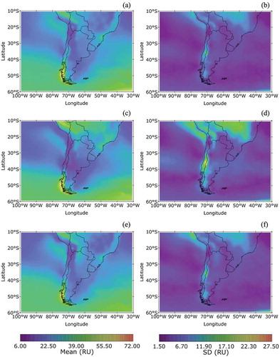
Figure 1. Continued.

In general, relative lower LER means are found over continental Argentina and their adjacent waters regardless of the season, with variability for these regions being low too. Storm track activity at these latitudes occurs throughout the year. The contours of relative vorticity and the associated track density in the lower troposphere follow the coastline, and in the upper troposphere/lower stratosphere, the track density reduces inland (Hoskins and Hodges 2005). These features suggest that the continental relative LER mean minima can be linked to the orography-forced asymmetry of the storm tracks (Inatsu and Hoskins 2004). LER means over 70 RU in the southern Andes are present all year long in a region with strong mountain wave activity (Eckermann and Preusse 1999; Pulido et al. 2013). Variability shows moderate values over this latter region, the highest of them taking place in JJA (Figure 1(h)). The Andes are much higher north of this region, approximately at 35°S, with the Aconcagua summit ranking among the highest points on Earth (6960 m, Pacino et al. 2014), only exceeded by several peaks in Asia (Lazio et al. 2010). Suitable environmental conditions for snow accumulation in JJA are hence warranted. LER means do account for this at least partially, as the highest (lowest) values in this region occur in JJA (DJF), with the caveat that they can also be related to the presence of cloudiness associated to enhanced gravity wave activity in both seasons (Yan 2010). The spring LER means being also high may respond either to wave activity (De La Torre et al. 2006) or to the snowmelt IA variability (Araneo and Compagnucci 2008), in particular through variability in the latter process. The prominent higher SDs over the region that are present throughout the year (Figure 1(b)) but has the highest values in DJF (Figure 1(d)) and in JJA (Figure 1(h)) can be explained by the aforementioned processes too.

LER mean maxima along the Brazilian coast are present across all seasons, likely tied to the forced ascent of the air caused by both Serra da Mantiqueira (SM) and Serra do Mar that run parallel to the coast (Almeida and Carneiro 1998). Persistent LER mean maxima also take place off the coasts of northern Chile and southern Peru, as seen from the annual climatology, and can be associated to high albedo stratocumuli (Eck et al. 1987; Kuang and Yung 2000; Serpetzoglou et al. 2008; references therein). A closer analysis reveals seasonality. The highest DJF LER means over the Peruvian Andes (PA) are in agreement with the establishment of a monsoonal circulation that lead to higher and colder cloud tops there (Vera et al. 2006). The high SD values represent the alternation between overcast and clear sky conditions over both continent and ocean, and these relative variability maxima extend along the coast down to 25°S. JJA has a variability pattern that is similar to the DJF one, but with high LER means shifted from the continent to the ocean. The MAM (Figures 1(e) and (f)) and SON (Figures 1(i) and (j)) pictures are similar in that they exhibit low means along the coastline with higher values to their east and west, whereas SDs are the highest over the ocean just south of 10°S.

Dubbed ‘the driest place on Earth’ (Fritz 2015), several factors conspire to make the Atacama Desert one of the most arid regions worldwide (Houston and Hartley 2003; Houston 2006). The Chilean portion of this desert has the lowermost LER values across all seasons. Furthermore, LER there virtually shows no deviations from its corresponding mean, making the skies in this area the clearest ones in the study region from a UV perspective. Lowermost LER values in the Atacama Desert and in northwestern Argentina (spanning the west of the provinces of Mendoza, Catamarca, La Rioja, Salta, and Jujuy) are simultaneous in SON. On the other hand, there exists a large area over tropical Brazil in JJA that has the season’s lowermost values, but they contrast with their higher DJF figures, a behaviour that is in agreement with a monsoon regime (Wang 1994). This region’s lower JJA climatological values (around 6 RU) are slightly over their recorded 2–3 RU albedoes (Kleipool et al. 2008), whereas they experience a fivefold increase in DJF. Variability in the region experienced a remarkable increase towards the equator in JJA. Hence, unusual overcast conditions, the sporadic presence of atmospheric aerosols, or both factors, make up the standing differences with the recorded albedoes.

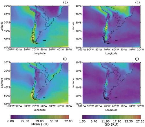
Two different kinds of loops of standardized seasonal anomalies were built in order to present the way LER values evolved within the study period. One of them is based on the Q grand-time means and variabilities (Figure S1). The other ones correspond to each season individually (Figures S2, S3, S4, and S5). In each case, the means and SDs used are the ones shown in Figure 1. Figure 2 shows a seasonal average over the maps of Figure S1. Overall, the DJF mean anomaly field (Figure 2(a)) is in agreement with Figure 1(c). Figure 2(b) shows a sign reversion in the JJA anomalies with respect to the DJF ones, and of the SON deviations (Figure 2(d)) with respect to the MAM ones (Figure 2(c)). Regarding DJF, the remarkable features are the highest anomalies over an area encompassing southern Peru, Bolivia, southern Brazil, and the associated northerly intrusion in northwestern Argentina. This intrusion is related to an enhancement of convective cloudiness due to the advection of moisture from the tropics (Nogués-Paegle and Mo 1997; Gan, Kousky, and Ropelewski 2004). Its main support is given by lee cyclogenesis (Wang and Fu 2004) and by a regional lower tropospheric low pressure system further south (Lichtenstein 1980). The extreme positive anomalies in DJF that extend along the east of the Andes in northwestern Argentina can be related to an enhancement of dynamic instability created by the concurrence of the subtropical jet (STJ), whose mean position locates over southern Bolivia/northern Argentina (Gan, Kousky, and Ropelewski 2004), and a latitudinal low level jet (LLJ) in the area (Wang and Fu 2004); the outstanding tongue-shaped anomalies are likely due to the latitudinal meanderings of the STJ. There is also a noticeable spot of positive anomalies around the Sierras de Córdoba (30°S, 65°W) whose presence has been proved to play a role in focusing convection (Rasmussen and Houze 2016). The spot of positive anomalies on the subtropical Pacific coast (30°S, 75°W) has a rather different origin. The similarity with the east of the Andes is that the region is under the influence of a southerly LLJ which is more frequent in late SON and in DJF (Garreaud and Muñoz 2005). The subtropical southeastern Pacific is dominated by large-scale subsidence within a semi-permanent anticyclone that sinks the air to create a subsidence inversion. However, the mean vertical velocity is upwards at the LLJ’s exit region. Figure 2 shows that increased positive anomalies there are in line with this. Their relative smaller anomalies when compared to the ones east of the Andes can be tied to less moisture availability given that the southerly LLJ flows over the cool surface waters of the Humboldt Current. DJF negative anomalies occur in the central portion of the study region, whereas positive anomalies dominate south of approximately 40°S in connection with the southernmost position of the storm tracks. Overall, Figure 2(a) resembles the DJF mean contours of OLR (Satyamurty, Nobre, and Silva Dias 1998, see their Figure 3C.3). In particular, the season’s tropical maxima anomalies can be attributed to deep convection in view of the associated cloudiness being related to OLR minima (Waliser, Graham, and Gautier 1993).

Figure 2. Seasonal mean values of standardized anomalies, calculated over the panels of Figure S1, for (a) DJF, (b) MAM, (c) JJA, and (d) SON.

In general, both lower anomalies and less contrasting values occur in the entire domain during MAM. An important exception is represented by an arch of maxima anomalies over northern Argentina (30°S, 60°W) that extends latitudinally and is shifted slightly to the east of its DJF counterpart. As in DJF, it can also be related to the dynamic instability created by the concurrence of the STJ and the LLJ, which is present throughout the year (Marengo et al. 2004; Wang and Fu 2004). Despite this, SON anomalies at the same region are less prominent than in MAM, possibly because of a lesser availability of moisture. Expectedly, the MAM and SON anomalies fields are generally the least distorted ones.

Anomalies in Figure S1 ranged from −4.13 to 5.25 across the study period. The lowermost values took place in SON 1978 over the Pacific Ocean (30°S, 75°W), in the centre of an area with low significant anomalies where the Pacific LLJ’s exit region locates, whereas the uppermost values occurred in southern Patagonia in JJA 1994. Apart from these two extreme cases, deviations from the long-term Q mean, such as the extreme positive anomalies in the southeastern Pacific in DJF 1994, the signal of a wave train between 50° and 60°S in JJA 2003, or the extreme positive deviations along the Central Andes in DJF 2012, are worth noting. Figure 3 shows the evolution of the percentages of positive and negative and of significant and not significant anomalies for each of the maps in Figure S1. Figure 3(a) shows an apparent increase in positive values since 1991. In order to evaluate the presence of any break in these time series, a shift-detecting algorithm based in Rodionov (2004) was carried out using mobile windows ranging between 2 and 6 years, i.e. eight and 24 consecutive seasons, respectively. The algorithm was set to skip the analysis for any mobile window if there was at least one missing value in the timescale involved. Results indicate that the positive anomalies indeed experienced an upward shift in JJA 1991 for the 3.25 and 3.50 years timescales. The long timescale had a shift slightly stronger than the short one; the mean upward shift was at around 32%. Unfortunately, longer timescales for this shift could not be evaluated owing to the algorithm’s skipping condition for missing data. Nevertheless, the 1991 shift was detectable enough to add to others found in the early 1990s in different variables (Barrucand, Rusticucci, and Vargas 2008; and references therein; Yu et al. 2015). By contrast, the time series of significant values (Figure 3(b)) shows no shifts at all.

Figure 3. Percentages of the total number of (a) positive and negative standardized anomalies in the study region for each of the seasons under analysis and (b) significant and not significant standardized anomalies for these seasons.

The deviations shown in Figures S2–S5 are IA and season specific. DJF anomalies (Figure S2) lay within the −2.40–4.85 range. The minimum values were recorded in 2012 over the southeastern Pacific (22.5°S, 77°W) and the maximum deviations took place in 1994 in an area slightly shifted southeastwards from the same region. The MAM anomalies (Figure S3) ranged between −3.13 and 3.44. The minimum values occurred in central Paraguay in 2003; the maximum values took place off the coasts of the Brazilian state of Bahia (BA) in 2009. The JJA anomalies (Figure S4) ranged between −3.31 and 5.19. The lowermost value took place in 1996 within a large area with negative anomalies covering northern Argentina, whereas the higher deviations were recorded in 1994 over the eastern portion of the Santa Cruz province, in the Argentine Patagonia. The SON anomalies (Figure S5) ranged between −3.81 and 3.50; they reached the lowermost values in 2015 in northeastern BA and the maximum anomalies were recorded in 1978 over the southwestern Atlantic, within a spot of significant values, located approximately at (50°S, 45°W) and enclosed by a greater area of non-significant positive deviations. It is hard to assess on the particular causes of the aforementioned seasonal extreme values due to the possible combination of several effects. Nonetheless, the DJF minima can be partly attributed to the PDO, as it coincides with the longest and strongest PDO negative phase of the last decades and the region shows a positive correlation with this index (see Section 3.3). Similarly, the strong 1997/98 El Niño can be recalled for the presence of positive anomalies in northeastern Argentina in DJF 1998 in agreement with the El Niño-related precipitation patterns in the region (Ropelewski and Halpert 1987).

A shift analysis on the time series of the total number of positive anomalies for the maps in Figures S2–S5 was carried out (not shown). The analysed timescales ranged from 3 to 10 years. At least one shift was recorded in all seasons. The shift analysis results are as follows.

1. There was a downward shift for the DJF series in 1984, with an average value of approximately −27% for two timescales involved (3 and 4 years).

2. There was an upward shift for the rest of the time series in 1991. The timescales involved for MAM, JJA, and SON led to average shifts of approximately 28% (3 and 4 years), 40% (4 years), and approximately 47% (3 and 4 years), respectively. Longer timescales could not be evaluated due to the restrictions imposed on the algorithm regarding missing data. As mentioned above, a shift in the early 1990s is in agreement with the existing literature.

3. There were two further upward shifts for JJA in 2004 and 2005. The former case comprises the 6–8 years timescales with an average shift of 23%. The latter case comprises a single timescale of 9 years, with a shift of approximately 21%.

4. MAM had two further upward shifts in 2005 and 2006. The timescales involved in the first case ranged from 3 to 8 years, with an average shift of around 21%. A single timescale (9 years) led to a shift of approximately 18% for the 2006 case.

The time series of significant values was analysed in a similar fashion. A single shift was recorded for them: it occurred in DJF 1984 for the shorter analysed timescale only, and it led to a shift of around 18%. This being the only detected shift in the time series of significant values and it taking place within a period with no sensor or satellite changes (i.e. it corresponds to the TOMS in the N7 campaign) is a result that strengthens its factuality. All in all, the contribution of the different sensors or satellites to all the aforementioned inhomogeneities cannot be completely ruled out.

3.2. Trends

A trend analysis was carried out on the LER mean seasonal values at each pixel in two different ways. Linear trends were estimated, and it was also checked whether there was a trend of any kind (i.e. not necessarily linear) using the Mann–Kendall test (see e.g. Motiee and McBean 2009). All these trends were statistically tested to a 95% of significance. Figure 4 shows the linear trend for both Q and IA cases. Q trends (Figure 4(a)) range between −0.04 and 0.10 RU season⁻¹ (i.e. between −1.60 and 4 RU decade⁻¹, respectively) if individual pixels are considered. There are 1906 pixels (out of 2800, or 68% of the domain) with a significant trend. Collectively, the pixels with the strongest significant negative and positive trends are located inland. The largest positive ones are found along the PA (approximately 3.20 RU decade⁻¹), whereas the largest negative (around −1.40 RU decade⁻¹) occur in southeastern Brazil in a region located between Serra do Espinhaço (SE) and the Chapada Diamantina (CD) and the coastline, spanning the easternmost portions of the states of Minas Gerais (MG) and BA. Another interesting feature is that most of the pixels over the oceans have a significant positive trend.

Figure 4. Trends in LER mean seasonal values within the study period for (a) Q, (b) DJF, (c) MAM, (d) JJA, and (e) SON. Values expressed in RU decade⁻¹. Significant values to a 95% confidence level are cross-hatched.

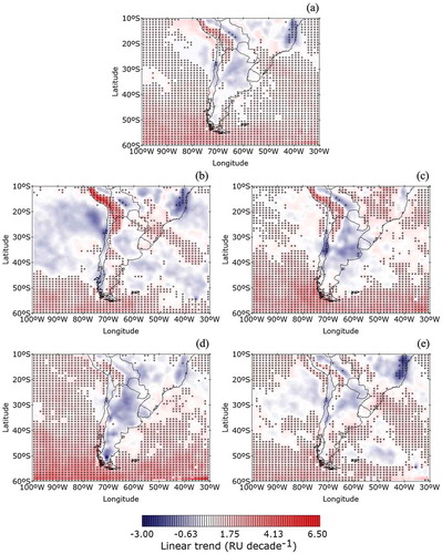
DJF (Figure 4(b)) has 918 pixels with a significant trend (33% of the total). The location of the largest significant trends replicates the Q ones along the PA and in the easternmost parts of MG and BA, positive in the former case (approximately 6 RU decade⁻¹) and negative in the latter one (around −1.70 RU decade⁻¹). Significant positive trends during the season are more numerous over the oceans and they are generally confined to latitudes beyond 45°S. A remarkable exception occurs in a northwest-by-southeast axis radiating from southern Brazil that is in juxtaposition with a band of moisture flux convergence (BMFC) due to the combination of several factors that lead to intense precipitation over the La Plata Basin (Silva and Berbery 2006). Positive trends here are in the order of 1.50 RU decade⁻¹. Even though trends were estimated in Herman et al. (2013), they did not calculate them on seasonal time series. However, the outcome of this work is qualitatively in agreement with theirs as most of the positive and negative trends are located over the oceans and land, respectively. One of the most remarkable differences is that we found no significant trends over the Pacific Ocean off the coasts of Chile and Peru, whereas Herman et al. (2013) did. By contrast, YLC found a positive trend at the same region; yet, they analysed a shorter period. These disparities highlight the sensitivity of trends to the different spacing and to the length of the input time series.

In MAM (Figure 4(c)), the number of pixels with a significant trend increases with respect to DJF to 1462 (52% of the domain), and there are a large number of oceanic pixels with a positive trend as well. The significant positive trends in the PA that extend south along the Andes to northwestern Argentina in DJF are also present in MAM; yet, they are weaker (approximately 3.5 RU decade⁻¹ at its maximum). Another region with positive trends is the Brazilian Highlands in southern Brazil, just over the area where there is a marked contrast between DJF and JJA due to the monsoon. Trends for this region, in the order of 1.50 − 2 RU decade⁻¹, can be interpreted as an indicator that the monsoon there is exceeding its canonical summer time frame and extends into the autumn in the last years. These results are in concordance with earlier findings (Marengo et al. 2009).

The point count with a significant trend in JJA (Figure 4(d)) is even higher than in MAM with 1737 pixels (62% of the domain). The majority of them are located over the oceans where their trend is positive, and the trend strength increases southwards. Generally, trends over the Pacific are stronger than over the Atlantic, particularly between 50° and 60°S. The Bolivian Andes and their surroundings also have a positive trend (in the order of 2 RU decade⁻¹). Although JJA seems to have the most number of negative trends, it also has the least concentration of significant ones.

The number of pixels with a significant trend in SON (Figure 4(e)) is 1354 (48% of the domain). As in DJF, significant negative anomalies (in the order of −2.5 RU decade⁻¹) are mostly concentrated east of MG and BA. Quite the rest of the significant trends occur in oceanic pixels and are positive. Two situations in the Atlantic basin are worth noting. The first one corresponds to the location of the BMFC in DJF. Pixels there, with a significant trend of 2 RU decade⁻¹ on average, span a larger area than in DJF. Given that the South Atlantic Convergence Zone (SACZ) develops in early summer (Satyamurty, Nobre, and Silva Dias 1998) and that the summer seesaw pattern in precipitation goes along with it (Silva and Berbery 2006), one possible explanation for the SON significant trends at the BMFC region relies upon an earlier advance of the processes that lead to the SACZ, particularly the southward migration of the sub-tropical high (Satyamurty, Nobre, and Silva Dias 1998), in line with a widening of the tropical belt (Eastman and Warren 2009; Birner 2010; and references therein). The second situation corresponds to the south of the province of Buenos Aires in Argentina, the only season exhibiting significance in the region.

By contrast to Figure 4, Figure S6 shows the pixels at which a trend of any kind was detected. The reciprocity between the corresponding maps in Figure 4 and S6 is striking, and such resemblance may imply an acceleration or deceleration in non-linear trends over the last years. Nevertheless, the study of non-linear trends is beyond the scope of the present work.

3.3. Correlations with circulation indices

In order to evaluate the possible linkages of the study variable with different global atmospheric processes, the Spearman’s correlation coefficient r between the standardized anomalies of seasonal LER values and of 14 global circulation indices were calculated. This coefficient establishes a relationship between the correlated variables through a monotonic function. A greater value of the absolute value of r links significant conditions of a given index to identifiable LER anomalies, so it is one way to address on the regional features of LER which are associated to particular states of the global atmosphere and its variability. The indices included in the analysis are the Dipole Mode Index (DMI, Saji et al. 1999; monthly values retrieved from http://www.jamstec.go.jp/frcgc/research/d1/iod/DATA/dmi.monthly.txt), the PDO (Mantua et al. 1997; monthly values retrieved from http://www.esrl.noaa.gov/psd/data/correlation/pdo.data), the Quasi-biennial Oscillation (QBO, Baldwin et al. 2001; monthly values retrieved from https://www.esrl.noaa.gov/psd/data/correlation/qbo.data), the Southern Oscillation Index (SOI, Ropelewski and Jones 1987; monthly values retrieved from http://www.cpc.ncep.noaa.gov/data/indices/soi), and the Madden-Julian Oscillation (MJO, Zhang 2005) at 10 different longitudes (data in pentads retrieved from http://www.cpc.ncep.noaa.gov/products/precip/CWlink/daily_mjo_index/proj_norm_order.ascii and seasonal means calculated thereof).

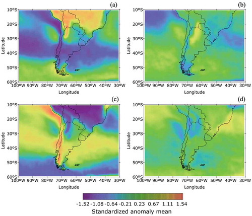
Figure 5 shows the values of r for the Q case. The correlation between the DMI and LER (Figure 5(a)) has significant r values at 1480 pixels (Table 1), or 53% of the domain. r is positive and located over the oceans with the exception of few negative values over MG and BA. The uppermost (lowermost) value of r in this case is 0.38 (−0.18). Regarding the PDO (Figure 5(b)), significant positive values of r occur over the continent in northern Argentina, whereas significant negative values take place over the oceans, with the largest concentration of such pixels in the Pacific, southwest of the landmass, and in the Atlantic, east of BA, where the lowermost values of r for this map are found. The number of pixels with significant values of r is less numerous in this case (15% of the domain) than in the DMI case; yet, the significant negative values are stronger (the uppermost and lowermost values in the PDO case are 0.29 and −0.32, respectively). Significant correlations with the QBO (Figure 5(c)) account for just 3% of the pixels, so the QBO does not seem to affect the region’s troposphere in the considered timescale.

Table 1. Number of pixels with a significant value of the Spearman’s correlation coefficient between LER and the specified indices.

Index		Q	DJF	MAM	JJA	SON
DMI		1480	261	743	447	862
PDO		424	184	237	268	132
QBO		87	43	104	60	121
SOI		761	471	275	708	559
MJO	20°E	109	45	80	190	73
	70°E	446	173	259	298	350
	80°E	533	286	324	314	468
	100°E	499	369	303	270	446
	120°E	263	292	148	55	437
	140°E	29	160	101	168	130
	160°E	375	72	127	305	268
	120°W	494	286	363	310	404
	40°W	456	353	289	225	432
	10°W	112	203	71	100	302

The total number of pixels in the study region is 2800.

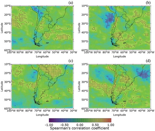
Figure 5. Spearman’s correlation coefficients between the Q standardized anomalies of LER and of (a) the DMI, (b) the PDO, (c) the QBO, (d) the SOI, (e) the MJO at 80°E, and (f) the MJO at 120°W. Significant values to a 95% confidence level are cross-hatched.

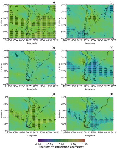
As to the SOI (Figure 5(d)), there are 761 points (27% of the domain) with significant correlations, most of them negative, whose lowest values occur over central Argentina. In this map, the uppermost and lowermost values of r are 0.25 and −0.39, respectively. The correlation pattern over the continent is in agreement with an increase of precipitation in the area during the negative phases of the index (El Niño) and a reduction of precipitation during the positive phase (La Niña) (Ropelewski and Halpert 1987; Ropelewski and Halpert 1989). The subtropical-to-mid-latitude Atlantic can be considered part of the same area. Furthermore, the correlation map shows other regions that are significantly linked to the SOI, most notably the exit region of the southerly LLJ off the Chilean coast and the region with strong mountain wave activity across the year further south, both with a direct relationship, and the subtropical Pacific west of 80°W, between 30° and 40°S, with negative correlations.

Even though the MJO is given at 10 different longitudes (20°E, 70°E, 80°E, 100°E, 120°E, 140°E, 160°E, 120°W, 40°W, and 10°W), it is not necessary to discuss the correlations with all these indices in view of the resemblance between some of them, which rely upon the different phases of the MJO across the Tropics (Zhang 2005). A map worth discussing is the one for the MJO at 80°E (Figure 5(e)), which can be interpreted as a teleconnection with convection whose core locates in eastern India. The map has the largest number of significant positive correlations (totalling 533 pixels, or 19% of the grid) and with no significant negative values for r. The uppermost value of r is 0.31. The map also noticeably resembles the SOI counterpart, in accordance with a direct relationship between the MJO and the SOI (Zhang 2005). Following this, the area covered by significant correlations is roughly the same as that for the SOI, with the exception of the eastern portion of the province of Buenos Aires, Uruguay, and adjacent waters. The exit region of the southerly LLJ off the coast of Chile is also excluded. The 80°E and 120°W (Figure 5(f)) correlation maps are spatially in resemblance but with an inverted polarity, in agreement with the MJO’s longitudinal phasing. By contrast to these two maps, the one for the MJO at 140°E (not shown) has the least number of significant correlations (Table 1).

The correlation maps for DJF, MAM, JJA, and SON are shown for the DMI, the SOI, and the MJO at 80°E (Figures 6–8, respectively). All these maps share two distinct characteristics with respect to the corresponding Q ones: extreme correlations are stronger and, in general, their significant values are circumscribed to certain areas. Concerning the DMI in DJF (Figure 6(a)), LER is significantly linked to it in 261 points (approximately 9% of the domain), mostly of them with a positive value of r and located mainly over the Drake Passage (DP) and surrounding waters. The number of significant pixels for the correlations in MAM (Figure 6(b)) increases to 743 (27% of the domain), with concentrations of positive values of r along the DP, the subtropical Pacific, the mid-latitude Atlantic, the subtropical Andes, over the eastern portions of MG and BA, and along and off the coasts of the Brazilian states of Espirito Santo (ES) and BA. In JJA (Figure 6(c)), the count of significant correlations is 447 (around 16% of the grid), most of them positive and with spots across the Pacific and even stronger values in the Atlantic between 30° and 40°S. The Andes also have a significant positive signal between these two latitudes, and a dipole locates over the coasts of BA and ES. SON (Figure 6(d)) has the most number of points with a significant correlation (862, or 31% of the domain). Most of them locate in the Atlantic south of 30°S and in the Argentine Patagonia south of 40°S. The Andes also have a significant signal between 10° and 40°S, along with a northwest-by-southeast diagonal in the Pacific between 30° and 40°S. On the other hand, significant negative correlations occur in the Pacific, approximately at 25°S, slightly north of the Chilean LLJ’s exit region, and over SM in Brazil. Excluding the negative values, the MAM and SON correlation patterns have a strong resemblance with the Q counterpart.

Figure 6. Spearman’s correlation coefficients between the standardized anomalies of LER and of the DMI for (a) DJF, (b) MAM, (c) JJA, and (d) SON. Significant values to a 95% confidence level are cross-hatched.

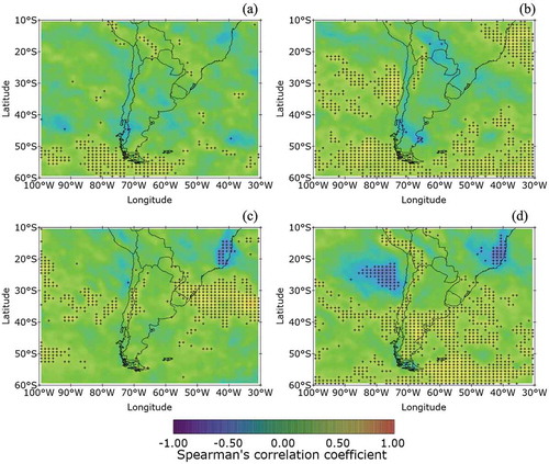
Figure 7. As in Figure 6 but for the standardized anomalies of LER and of the SOI.

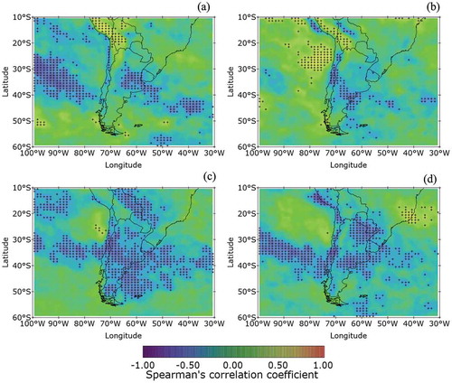
Figure 8. As in Figure 6 but for the standardized anomalies of LER and of the MJO at 80°E.

The SOI in DJF (Figure 7(a)) has 471 pixels with significant correlation (17% of the domain), the majority of which are negative. There are two regions with the most number of contiguous points in such condition, namely the Pacific between 30° and 40°S and central-eastern Argentina, whose significant negative correlations extend southeast to also include the Atlantic along 40°S. These two regions were also present in the Q case; yet, the former (latter) one spans a larger (smaller) area in the summertime. On the other hand, the largest number of positive correlations occurs in the Peruvian and the Bolivian Andes (PBA). There is a resemblance between the SOI and the correlation map associated to the MJO at 80°E with an inverted polarity (Figure 8(a)). Regarding MAM (Figure 7(b)), there are 275 pixels (or roughly 10% of the total) with significant r values. The main concentration of significant positive correlations occur over the PBA and off the Chilean coast between 20° and 30°S, approximately in the LLJ’s exit region. The largest number of contiguous significant negative correlations extend from northern Chile to the northeastern Patagonia in Argentina, approximately along the so-called dry diagonal (Houston and Hartley 2003; Garreaud 2009) between 20° and 40°S, extending eastwards approximately along the latter latitude, from 70° to 60°W. As in DJF, the correlation map with the SOI has a resemblance with the one for the MJO at 80°E (Figure 8(b)) but with an indirect polarity. However, the number of pixels that have a significant correlation with the MJO at 80°E exceeds the one for the SOI since it includes additional spots in the Atlantic Ocean.

The most striking SOI/LER relationship takes place in JJA (Figure 7(c)) when the number of points with significant values rises to 708 (or a quarter of the domain). During this season, significant negative correlations cover the continent, south of 25°S, almost entirely, with the exception of southern Brazil and Uruguay. Also included as part of the same area are the adjacent waters of the Atlantic and the Pacific along 30°S. Since negative (positive) values of the SOI are associated to ENSO warm (cold) events, a negative (positive) correlation implies a direct (indirect) relationship between ENSO warm (cold) events and cloudiness or snow. The STJ, which constitutes a known source for cyclogenesis processes especially at their polar flank (Hoskins and Hodges 2005), reaches its southernmost position during this season (see e.g. Garreaud 2009). Needless to say, even though the ENSO plays an important role in South America’s IA variability (Satyamurty, Nobre, and Silva Dias 1998), it is not the only forcing. Hence, the results just partly tie the ENSO forcings to cyclogenesis processes in the region, in view of the close connection between cyclogenesis and cloudiness. There is another region of significant adjoining points between 10° and 20°S that span the Bolivian lowlands, southwestern Brazil, and northern Paraguay. As a matter of fact, precipitation in the Bolivian portion of this area has a maximum in summer; yet, winter amounts are less important but still sizeable owing to the advection of cold air along the Andes (Ronchail et al. 2002). Results for this region regarding ENSO cold events during JJA are quite in agreement with the existing literature as drier conditions (i.e. less cloudiness) are expected. As for ENSO warm events, the signal in precipitation is not as strong and seems to rely upon a number of regional factors. The similarity between the correlation maps of the SOI and the MJO at 80°E is just partial in this season as significant correlations over the continent south of 20°S vanishes (Figure 8(c)).

The number of points with a significant correlation with the SOI reduces to 559 (or 20% of the domain) for SON (Figure 7(d)). Expectedly, the correlation map for this season resembles its JJA counterpart due to the thermal inertia in both oceans (e.g. Hoskins and Hodges 2005), and in the ENSO as a global process as well. Nonetheless, significance spans a reduced area but there are a greater number of spots with adjoining significant pixels. Three are the major regions with contiguous significant negative values of r. The most noticeable one lies between 30° and 40°S. It extends between 100° and 50°W forming a ‘U’ shape, with a disruption in significance over the Andes. Considering that ENSO plays an important role in South America’s IA variability and that all these maps show the relationships between the SOI and cloudiness, this disruption may be related to reinforcements in both decay of the systems upstream of the Andes and their regeneration downstream of the topography during ENSO warms events. This hypothesis is supported by below average geopotential heights in the lower atmosphere during ENSO warm events (Aceituno 1989). The other two regions with adjoining significant negative correlations are northern Argentina and southern Paraguay (NASP), which again can be related to more intense cyclogenesis during ENSO warm events due to a strengthened STJ (Kousky, Kagano, and Cavalcanti 1984; Aceituno 1989), and northern Chile and the southern Peru coastline. By contrast, there exists just one area with significant positive correlations that is located east of SM, centred over the Brazilian state of Rio de Janeiro (RJ). This region and NASP define a dipole in correlations that is quite in agreement with Kousky and Cavalcanti’s (1988) OLR spatial ‘seesaw’ pattern of their fourth rotated empirical orthogonal function, with the associated time series being mostly positive during ENSO warm events, most notably during the 1982/83 warm episode. Again, there is a resemblance between the correlation maps of the SOI and the MJO at 80°E (Figure 8(d)) in that they share the same regions but with opposite polarity; yet, the number of pixels with significant correlations (468 for the MJO at 80°E, cf. Table 1) is smaller than the SOI one.

As to the PDO, in DJF (Figure S7(a)), the number of significant correlations decreases to 184 (approximately 7% of the domain) when compared with the Q case. Even though there are scattered spots of positive and negative r values, the region with the largest concentration of positive correlations lies in the subtropical Pacific, in the stratocumulus region off the Chilean and the Peruvian coasts. On the other hand, the largest number of negative correlations concentrates off the coasts of BA and ES in a region that presents correlations of the same kind in the Q case but with stronger values during the summertime. MAM (Figure S7(b)) has 237 pixels (around 8% of the domain) with significant correlations, whose values are predominantly negative and mostly concentrated in two regions: approximately over the Chilean LLJ’s region of influence and to the south-westernmost tip of the landmass. These two areas match the ones for the DMI but with an opposite polarity in correlations. The number of pixels with significant values of r in JJA (Figure S7(c)) is slightly over the one in MAM, but they are much more scattered. Negative values dominate with the largest concentration of them located over the Pacific, approximately at 95°W between 40° and 50°S. SON (Figure S7(d)) has the least number of significant correlations. The most remarkable feature for this season is the thin line of significant positive values of r in the Peruvian coast that extend into the south along the subtropical Andes between 20° and 40°S.

The index used here to represent the QBO is the zonal mean of the 30 hPa wind at the Equator. Strong easterlies at the Equator define a negative anomaly or the east phase, whereas weak easterlies or westerlies lead to the west phase. The QBO has a relatively small number of significant r values across all seasons (Table 1). The most number of adjoining points with significant correlations occur in SON (Figure S8(d)) off the Chilean and the Peruvian coasts, in a stratocumulus-prone region (Klein and Hartmann 1993; Corbo and Weller 2007) and in MAM (Figure S8(b)) over the DP and east of it. The prominent signal at the two aforementioned seasons in the regions specified is worth noting. In particular, in the SON case, the stratocumulus region overlaps with the equatorial eastern Pacific upwelling zone, whose variability is strongly tied to the ENSO. This could be related to the known ENSO/QBO entanglement (Baldwin et al. 2001, and references therein), but the LER/SOI correlations at the same region are not significant. Hence, the SON signal is strictly related to the QBO. The correlations in both MAM and SON are negative, i.e. more (less) cloudiness in these regions is expected for the QBO east (west) phase. Since the QBO is the only used index that includes information from the stratosphere, these results show an apparent teleconnection between the tropical stratosphere and the troposphere. Research efforts linking the equatorial stratospheric QBO with the extratropical troposphere are scarce in the Northern Hemisphere (see e.g. Coughlin and Tung 2001; Ruzmaikin et al. 2005) and it is a vacant topic in the SH to the best of our knowledge.

4. Summary and concluding remarks

A UV LER climatology for southern South America was introduced. The study region comprised the area limited by 10° and 60°S and 30° and 100°W. The period of analysis was 1978–2015 including data collected from TOMS instruments aboard three different satellites and the OMI on board the Aura spacecraft. Across the study period, seasonal means at each pixel were calculated for DJF, MAM, JJA, and SON. Long-term means and variabilities were derived thereupon on Q and IA bases. In view of the usefulness of LER as a proxy for cloudiness, most of the features of the mean and the variability fields could be attributed to atmospheric and oceanic processes of local, regional, or global origin which lead to the formation or to the presence of clouds of any kind.

An algorithm for the detection of breaks was applied to the Q and the IA time series of both positive and significant standardized anomalies. As to the Q time series, a 32% strong upward shift in positive values was detected in winter 1991. By contrast, the time series of significant values showed no breaks at all. As to the IA time series, the single downward shift took place in summer 1984 with strength of 27%. The rest of the detected breaks in positive anomalies had an upward shift. They occurred in all the seasons with the exception of DJF. In particular, the 1991 break affected MAM, JJA, and SON. In addition, there were shifts in the mid-2000s that generally spanned timescales closer to the decade, which had an influence in the MAM and JJA values. Separately, a single shift was detected for the DJF significant values in 1984.

A linear trend analysis on the mean seasonal values revealed that, on a Q basis, most of the pixels exhibiting a significant trend were located over the oceans and had an upward trend. However, the strongest trends were located over mountainous terrain, along the PA for the positive values (approximately 3.20 RU decade⁻¹) and in southeastern Brazil, in the portion of land located between the SE and the CD and the coastline for the negative ones (around −1.40 RU decade⁻¹). In the IA case, summer replicates the location of the regions with extreme values of the trends but with stronger figures (6 and −1.70 RU decade⁻¹). A remarkable feature is the presence of significant positive trends (in the order of 1.50 RU decade⁻¹) in a BMFC along a northwest-by-southeast axis over the subtropical Atlantic. As to MAM, the significant positive trends in the Brazilian Highlands (1.50–2 RU decade⁻¹), over a region that has monsoonal characteristics, are worth noting. The result was ascribed to an extension of the monsoonal conditions into autumn. Significant positive trends along the PA were also present during the season, with weaker values though (3.50 RU decade⁻¹ at most). Oceanic pixels aside, the most noticeable feature of JJA is the vanishing of significance over the central PA, whereas positive trends over the Andes in southern Peru and Bolivia are still significant but they have a weaker intensity than in MAM (2 RU decade⁻¹ at most). In SON, the significant negative trends east of SE and CD (with maximum values in the order of −2.50 RU decade⁻¹) and the positive trends along the BMFC region, covering a larger area than in DJF with a trend of 2 RU decade⁻¹ on average, are the two remarkable features of the season.

Linkages between LER and general circulation indices were addressed by means of the Spearman’s correlation coefficient between the standardized anomalies of both variables. The indices included in the analysis were the DMI, the PDO, the QBO, the SOI, and the MJO. The Q correlations are generally smaller than the IA ones. On a Q basis, the DMI seems to have a direct influence (i.e. positive values of the DMI are associated to more cloudiness) on both oceans and in central Argentina. The correlation pattern for the SOI is in agreement with an increase (decrease) in precipitation during El Niño (La Niña) events over an area covering central Argentina and the subtropical-to-mid-latitude Atlantic. The SOI also has a signal in the subtropical Pacific and in the exit region of the southerly LLJ off the subtropical Chilean coast. The correlation pattern for the MJO at some latitudes is similar to that of the SOI but with a direct or inverted polarity. This responds both to known relationships between the MJO and the SOI and to the longitudinal phasing of the MJO. On the other hand, the QBO does not seem to have a notable effect in the troposphere given the small number of pixels with a significant correlation.

Interannually, the aestival relationship between LER and the DMI is positive and it occurs in a major area located over the DP and its surroundings. Significance includes the DP also in MAM, along with the subtropical Pacific, the mid-latitude Atlantic, the subtropical Andes, and southeastern Brazil, with positive correlations in all these cases. The strongest positive correlations during JJA occur in the subtropical Atlantic. Spots of positive correlations are present in the subtropical Pacific and in the Andes between 30° and 40°S, and there is a dipole of correlations over the southeastern Brazilian coast, with negative values situated inland. The most number of significant positive correlations occur in SON, most of them located in the Atlantic beyond 30°S and over continental Argentina south of 40°S, whereas significant negative correlations are found north of the southerly LLJ’s exit region in the Pacific and over SM in Brazil.

Regarding the PDO, the regions with the summertime most concentration of contiguous significant positive and negative values are the stratocumulus region in the Pacific and the coasts of the Brazilian states of ES and BA, respectively. The Pacific presents the most number of autumntime significant negative correlations, with two loci of maxima correlations situated in the area of influence of the Chilean LLJ and further south, in the south-westernmost tip of the continent. These two regions also have a signal with the DMI but with opposite polarity. Negative values dominate the JJA correlations field, with the most concentration of significant values centred at 45°S and 95°W. SON has the least number of significant correlations, with the most notable feature being the thin line of positive values extending from 20° to 40°S along the Andes. In the Q case, the QBO has a relatively small number of pixels with a significant correlation and something similar occurs for each season on an IA basis. However, the large areas covered by significant negative correlations over the DP and east of it in MAM, and in the Pacific stratocumulus region in SON, are worth noting.

Unlike other indices, the SOI has an important signal in the study region on both Q and IA bases. In the first case, most of the significant correlations are negative. There is a major region, encompassing central Chile, central-eastern Argentina, and the subtropical-to-mid-latitude Atlantic, whose significant negative correlations are in agreement with known precipitation patterns associated to El Niño. A more reduced area of contiguous significant negative correlations spans the Pacific west of 80°W, between 30° and 40°S. On the other hand, significant positive correlations occur in the Pacific LLJ’s exit region and in the south-westernmost portion of the continent where there is strong wave activity all year round. In DJF, the most number of contiguous significant positive correlations occur in the PBA, whereas the Pacific west of 80°W and central Argentina also present significant negative correlations, but with a larger (smaller) extension that in the Q case for the former (latter) region. The PBA also present significant positive correlations in MAM, whereas the largest concentration of significant negative anomalies during the season extends from northern Chile down to the Argentine Patagonia along the dry diagonal. The overall largest concentration of significant negative correlations occurs in JJA, with the continent south of 25°S being almost entirely covered by them, a result partly tied to cyclogenesis processes. There is another region with such negative correlations spanning eastern Bolivia, southwestern Brazil, and northern Paraguay. The correlation maps for JJA and SON are quite in resemblance given the thermal inertia in both oceans, as well as in the ENSO-related processes. Three are the major spots with adjoining significant negative correlations in springtime: a subtropical band spanning the Pacific and central Argentina with a disruption over the Andes, NASP, and northern Chile and the Peruvian coastline. A single area of significant positive correlations occurs over the Brazilian state of RJ. This region and NASP define a dipole in significant correlations that is in concordance with a seesaw pattern in the OLR. As in the Q case, the correlation maps for the MJO defined at some longitudes are similar to the SOI counterparts.

The present study was carried out by complementing the LER database that was used in YLC up to 2015. The study area was reduced to southern South America and adjacent waters in order to assess the behaviour of the variable regionally and to link it to known atmospheric and oceanic processes that have an impact in the region. In spite of including the contribution of aerosols and snow, the presented climatology has generally been linked to processes that lead to the formation or maintenance of clouds. The potential for LER as both a diagnostic and a forecast variable can be further exploited by analysing shorter timescales (e.g. monthly or daily), by studying cloud types discretionally, or by combining the variable with others of relevance. All these topics are a matter of future investigation.

Acknowledgements

We are indebted to two anonymous reviewers for their comments and suggestions; they helped improving the original manuscript in many ways. We would also like to thank PIP 2012-2014 No. 0075, PICT 2012-2927, and PIDDEF 2014 No. 26 grants.

Disclosure statement

No potential conflict of interest was reported by the authors.

Supplemental data for this article can be accessed here.

Additional information

Funding

This work was supported by the Consejo Nacional de Investigaciones Científicas y Técnicas: [Grant Number PIP 2012-2014 0075], Fondo para la Investigación Científica y Tecnológica: [Grant Number PICT-2012-2927], and Ministerio de Defensa: [Grant Number PIDDEF 26/2014].

References

- Aceituno, P. 1989. “On the Functioning of the Southern Oscillation in the South American Sector. Part II: Upper-Air Circulation.” Journal of Climate 2: 341–355. doi:10.1175/1520-0442(1989)002<0341:OTFOTS>2.0.CO;2.
- Almeida, F. F. M. de., and C. D. R. Carneiro. 1998. “Origem E Evolução Da Serra Do Mar.” Revista Brasileria De Geociências 28 (2): 135–150.
- Araneo, D. C., and R. H. Compagnucci. 2008. “Atmospheric Circulation Features Associated to Argentinean Andean Rivers Discharge Variability.” Geophysical Research Letters 35: L01805. doi:10.1029/2007GL032427.
- Arking, A. 1991. “The Radiative Effects of Clouds and Their Impact on Climate.” Bulletin of the American Meteorological Society 71 (6): 795–813. doi:10.1175/1520-0477(1991)072<0795:TREOCA>2.0.CO;2.
- Baldwin, M. P., L. J. Gray, T. J. Dunkerton, K. Hamilton, P. H. Haynes, W. J. Randel, J. R. Holton et al. 2001. “The Quasi-Biennial Oscillation.” Reviews of Geophysics 39 (2): 179–229. doi:10.1029/1999RG000073.
- Barrucand, M., M. Rusticucci, and W. Vargas. 2008. “Temperature Extremes in the South of South America in Relation to Atlantic Ocean Surface Temperature and Southern Hemisphere Circulation.” Journal of Geophysical Research 113: D20111. doi:10.1029/2007JD009026.
- Birner, T. 2010. “Recent Widening of the Tropical Belt from Global Tropopause Statistics: Sensitivities.” Journal of Geophysical Research 115: D23109. doi:10.1029/2010JD014664.
- Boucher, O., D. Randall, P. Artaxo, C. Bretherton, G. Feingold, P. Forster, V.-M. Kerminen, et al. 2013. “Clouds and Aerosols.” In Climate Change 2013: The Physical Science Basis. Contribution of Working Group I to the Fifth Assessment Report of the Intergovernmental Panel on Climate Change, edited by T. F. Stocker, D. Qin, G.-K. Plattner, M. Tignor, S. K. Allen, J. Boschung, A. Nauels, Y. Xia, V. Bex, and P. M. Midgley, 571–657. Cambridge: Cambridge University Press.
- Buchard, V., C. Brogniez, F. Auriol, B. Bonnel, J. Lenoble, A. Tanskanen, B. Bojkov, and P. Veefkind. 2008. “Comparison of OMI Ozone and UV Irradiance Data with Ground-Based Measurements at Two French Sites.” Atmospheric Chemistry and Physics 8 (2): 4517–4528. doi:10.5194/acp-8-4517-2008.
- Charlson, R. J., A. S. Ackerman, F. A.-M. Bender, T. L. Anderson, and Z. Lui. 2007. “On the Climate Forcing Consequences of the Albedo Continuum between Cloudy and Clear Air.” Tellus 59 (4): 715–727. doi:10.1111/j.1600-0889.2007.00297.x.
- Charlson, R. J., S. E. Scwartz, J. M. Hales, R. D. Cess, J. A. Coakley, J. E. Hansen Jr., and D. J. Hofmann. 1992. “Climate Forcing by Anthropogenic Aerosols.” Science 255 (5043): 423–430. doi:10.1126/science.255.5043.423.
- Corbo, K., and R. Weller. 2007. “The Variability and Heat Budget of the Upper Ocean under the Chile-Peru Stratus.” Journal of Marine Research 65: 607–637. doi:10.1357/002224007783649510.
- Coughlin, K., and -K.-K. Tung. 2001. “QBO Signal Found at the Extratropical Surface through Northern Annular Modes.” Geophysical Research Letters 28 (24): 4563–4566. doi:10.1029/2001GL013565.
- Damiani, A., R. R. Cordero, J. Carrasco, S. Watanabe, M. Kawamiya, and V. E. Lagun. 2015. “Changes in the UV Lambertian Equivalent Reflectivity in the Southern Ocean: Influence of Sea Ice and Cloudiness.” Remote Sensing of Environment 169: 75–92. doi:10.1016/j.rse.2015.07.030.
- Damiani, A., R. R. Cordero, S. Cabrera, M. Laurenza, and C. Rafanelli. 2014. “Cloud Cover and UV Index Estimates in Chile from Satellite-Derived and Ground-Based Data.” Atmospheric Research 138: 139–151. doi:10.1016/j.atmosres.2013.11.006.
- De La Torre, A., P. Alexander, P. Llamedo, C. Menéndez, T. Schmidt, and J. Wickert. 2006. “Gravity Waves above the Andes Detected from GPS Radio Occultation Temperature Profiles: Jet Mechanism?” Geophysical Research Letters 33: L24810. doi:10.1029/2006GL027343.
- Dobber, M. R., R. J. Dirksen, P. F. Levelt, G. H. J. Van Den Oord, R. H. M. Voors, Q. Kleipool, G. Jaross et al. 2006. “Ozone Monitoring Instrument Calibration.” IEEE Transactions on Geoscience and Remote Sensing 44 (5): 1209–1238. doi:10.1109/TGRS.2006.869987.
- Eastman, R., and S. G. Warren. 2009. “A 39-Yr Survey of Cloud Changes from Land Stations Worldwide 1971− 2009: Long-Termtrends, Relation to Aerosols, and Expansion of the Tropical Belt.” Journal of Climate 26: 1286–1303. doi:10.1175/JCLI-D-12-00280.1.
- Eck, T. F., P. K. Bhartia, P. H. Hwang, and L. L. Stowe. 1987. “Reflectivity of Earth’s Surface and Clouds in Ultraviolet from Satellite Observations.” Journal of Geophysical Research 92 (D4): 4287–4296. doi:10.1029/JD092iD04p04287.
- Eckermann, S. D., and P. Preusse. 1999. “Global Measurements of Stratospheric Mountain Waves from Space.” Science 286: 1534–1537. doi:10.1126/science.286.5444.1534.
- Fritz, A. 2015. “The ‘Driest Place on Earth’ Is Covered in Pink Flowers after a Crazy Year of Rain.” The Washington Post, October 29. Accessed 10 October 2017. https://www.washingtonpost.com/news/capital-weather-gang/wp/2015/10/29/the-driest-place-on-earth-is-covered-in-pink-flowers-after-a-crazy-year-of-rain/
- Gan, M. A., V. E. Kousky, and C. F. Ropelewski. 2004. “The South America Monsoon Circulation and Its Relationship to Rainfall over West-Central Brazil.” Journal of Climate 17: 47–66. doi:10.1175/1520-0442(2004)017<0047:TSAMCA>2.0.CO;2.
- Garreaud, R. D. 2009. “The Andes Climate and Weather.” Advances in Geosciences 22: 3–11. doi:10.5194/adgeo-22-3-2009.
- Garreaud, R. D., and R. C. Muñoz. 2005. “The Low-Level Jet off the West Coast of Subtropical South America: Structure and Variability.” Monthly Weather Review 133: 2246–2261. doi:10.1175/MWR2972.1.
- Ghan, S. J., X. Liu, R. C. Easter, R. Zaveri, P. J. Rasch, J.-H. Yoon, and B. Eaton. 2012. “Toward a Minimal Representation of Aerosols in Climate Models: Comparative Decomposition of Aerosol Direct, Semidirect, and Indirect Radiative Forcing.” Journal of Climate 25: 6461–6476. doi:10.1175/JCLI-D-11-00650.1.
- Hansen, J., M. Sato, A. Lacis, and R. Ruedy. 1997. “The Missing Climate Forcing.” Philosophical Transactions of the Royal Society B: Biological Sciences 352: 231–240. doi:10.1098/rstb.1997.0018.
- Herman, J., M. T. DeLand, L.-K. Huang, G. Labow, D. Larko, S. A. Lloyd, J. Mao, W. Qin, and C. Weaver. 2013. “A Net Decrease in the Earth’s Cloud, Aerosol, and Surface 340nm Reflectivity during the past 33 Yr (1979–2011).” Atmospheric Chemistry and Physics 13: 8505–8524. doi:10.5194/acp-13-8505-2013.
- Herman, J. R., and E. A. Celarier. 1997. “Earth Surface Reflectivity Climatology at 340−380 Nm from TOMS Data.” Journal of Geophysical Research 102 (D23): 28003–28011. doi:10.1029/97JD02074.
- Herman, J. R., N. Krotkov, E. Celarier, D. Larko, and G. Labow. 1999. “Distribution of UV Radiation at the Earth’s Surface from TOMS-measured UV-backscattered Radiances.” Journal of Geophysical Research 104 (D10): 12059–12076. doi:10.1029/1999JD900062.
- Herman, J. R., P. K. Bhartia, A. J. Krueger, R. D. McPeters, C. G. Wellemeyer, C. J. Seftor, G. Jaross, et al. 1996. Meteor−3 Total Ozone Mapping Spectrometer (TOMS) Data Products User’s Guide. NASA Reference Publication 1939. Greenbelt, MD. ftp://toms.gsfc.nasa.gov/pub/meteor3/METEOR3_USERGUIDE.PDF
- Hess, M., P. Koepke, and I. Schult. 1998. “Optical Properties of Aerosols and Clouds: The Software Package OPAC.” Bulletin of the American Meteorological Society 79 (5): 831–844. doi:10.1175/1520-0477(1998)079<0831:OPOAAC>2.0.CO;2.
- Hoskins, B. J., and K. I. Hodges. 2005. “A New Perspective on Southern Hemisphere Storm Tracks.” Journal of Climate 18: 4108–4129. doi:10.1175/JCLI3570.1.
- Houston, J. 2006. “Variability of Precipitation in the Atacama Desert: Its Causes and Hydrological Impact.” International Journal of Climatology 26: 2181–2198. doi:10.1002/joc.1359.
- Houston, J., and A. J. Hartley. 2003. “The Central Andean West-Slope Rainshadow and Its Potential Contribution to the Origin of Hyper-Aridity in the Atacama Desert.” International Journal of Climatology 23: 1453–1464. doi:10.1002/joc.938.
- Inatsu, M., and B. J. Hoskins. 2004. “The Zonal Asymmetry of the Southern Hemisphere Winter Storm Tracks.” Journal of Climate 17: 4882–4892. doi:10.1175/JCLI-3232.1.
- Karoly, D. J., D. G. Vincent, and J. M. Schrage. 1998. “General Circulation.” In Meteorology of the Southern Hemisphere, edited by D. J. Karoly and D. G. Vincent, 47–85. Boston: American Meteorological Society.
- Kaufman, Y. J., and R. S. Fraser. 1997. “Confirmation of the Smoke Particles Effect on Clouds and Climate.” Science 277 (5332): 1636–1639. doi:10.1126/science.277.5332.1636.
- Klein, S. A., and D. L. Hartmann. 1993. “The Seasonal Cycle of Low Stratiform Clouds.” Journal of Climate 6: 1587–1606. doi:10.1175/1520-0442(1993)006<1587:TSCOLS>2.0.CO;2.
- Kleipool, Q. L., M. R. Dobber, J. F. De Haan, and P. F. Levelt. 2008. “Earth Surface Reflectance Climatology from 3 Years of OMI Data.” Journal of Geophysical Research (113): D18308. doi:10.1029/2008JD010290.
- Kousky, V. E., and I. F. A. Cavalcanti. 1988. “Precipitation and Atmospheric Circulation Anomaly Paterns in the South American Sector.” Revista Brasileira De Meteorologia 3: 199–206.
- Kousky, V. E., M. T. Kagano, and I. F. A. Cavalcanti. 1984. “A Review of the Southern Oscillation: Oceanic-Atmospheric Circulation Changes and Related Rainfall Anomalies.” Tellus 36A: 490–504. doi:10.1111/j.1600-0870.1984.tb00264.x.
- Kuang, Z., and Y. L. Yung. 2000. “Reflectivity Variations off the Peru Coast: Evidence for Indirect Effect of Athropogenic Sulphate Aeroslos on Clouds.” Geophysical Research Letters 27 (16): 2501–2504. doi:10.1029/2000GL011376.
- Labow, G. J., J. R. Herman, L.-K. Huang, S. A. Lloyd, M. T. DeLand, W. Qin, J. Mao, et al. 2011. “Diurnal Variation of 340 Nm Lambertian Equivalent Reflectivity Due to Clouds and Aerosolos over Land and Oceans.” Journal of Geophysical Research 116: D11202. doi:10.1029/2010JD014980.
- Lamb, P. J., and R. A. Peppler. 1987. “North Atlantic Oscillation: Concept and Application.” Bulletin of the American Meteorological Society 68 (10): 1218–1225. doi:10.1175/1520-0477(1987)068<1218:NAOCAA>2.0.CO;2.
- Lazio, M. P., J. D. Van Roo, C. Pesce, S. Malik, and D. M. Courney. 2010. “Postexercise Peripheral Oxygen Saturation after Completion of the 6-Minute Walk Test Predicts Successfully Reaching the Summit of Aconcagua.” Wilderness & Environmental Medicine 21 (4): 309–317. doi:10.1016/j.wem.2010.09.003.
- Levitus, S., J. I. Antonov, J. Wang, T. L. Delworth, K. W. Dixon, and A. J. Broccoli. 2001. “Anthropogenic Warming of Earth’s Climate System.” Science 292 (5515): 267–270. doi:10.1126/science.1058154.
- Lichtenstein, E. R. 1980. “La depresión del Noroeste argentino (The north-western Argentina low pressure area).” PhD diss., Universidad de Buenos Aires (In Spanish, abstract in English)
- Liepert, B. G., J. Feichter, U. Lohmann, and E. Roeckner. 2004. “Can Aerosols Spin down the Water Cycle in a Warmer and Moister World.” Geophysical Research Letters 31: L06207. doi:10.1029/2003GL019060.
- Lohmann, U., and J. Feichter. 2005. “Global Indirect Aerosol Effects: A Review.” Atmospheric and Chemistry Physics 5: 715–737. doi:10.5194/acp-5-715-2005.
- Mantua, N. J., S. R. Hare, Y. Zhang, J. M. Wallace, and R. C. Francis. 1997. “A Pacific Interdecadal Climate Oscillation with Impacts on Salmon Production.” Bulletin of the American Meteorological Society 78 (6): 1069–1079. doi:10.1175/1520-0477(1997)078<1069:APICOW>2.0.CO;2.
- Marengo, J. A., R. Jones, L. M. Alves., and M. C. Valverde. 2009. “Future Change of Temperature and Precipitation Extremes in South America as Derived from the PRECIS Regional Climate Modeling System.” International Journal of Climatology 29: 2241–2255. doi:10.1002/joc.1863.
- Marengo, J. A., W. R. Soares, C. Saulo, and M. Nicolini. 2004. “Climatology of the Low-Level Jet East of the Andes as Derived from the NCEP−NCAR Reanalyses: Characteristics and Temporal Variability.” Journal of Climate 17 (12): 2261–2280. doi:10.1175/1520-0442(2004)017<2261:COTLJE>2.0.CO;2.
- McPeters, R. D., P. K. Bhartia, A. J. Krueger, J. R. Herman, B. M. Schlesinger, C. G. Wellemeyer, C. J. Seftor, et al. 1996. Nimbus−7 Total Ozone Mapping Spectrometer (TOMS) Data Products User’s Guide. NASA Reference Publication 1384. Greenbelt, MD. ftp://toms.gsfc.nasa.gov/pub/nimbus7/NIMBUS7_USERGUIDE.PDF
- McPeters, R. D., P. K. Bhartia, A. J. Krueger, J. R. Herman, C. G. Wellemeyer, C. J. Seftor, G. Jaross, et al. 1998. Earth Probe Total Ozone Mapping Spectrometer (TOMS) Data Products User’s Guide. NASA Reference Publication 206895. Greenbelt, MD. ftp://toms.gsfc.nasa.gov/pub/eptoms/EARTHPROBE_USERGUIDE.PDF
- Motiee, H., and E. McBean. 2009. “An Assessment of Long-Term Trends in Hydrologic Components and Implications for Water Levels in Lake Superior.” Hydrology Research 40 (6): 564–579. doi:10.2166/nh.2009.061.
- Newman, M., M. A. Alexander, T. R. Ault, K. M. Cobb, C. Deser, E. Di Lorenzo, N. J. Mantua, et al. 2016. “The Pacific Decadal Oscillation, Revisited.” Journal of Climate 29 (12): 4399–4427. doi:10.1175/JCLI-D-15-0508.1.
- Nogués-Paegle, J., and K. C. Mo. 1997. “Alternating Wet and Dry Conditions over South America during Summer.” Monthly Weather Review 125: 279–291. doi:10.1175/1520-0493(1997)125<0279:AWADCO>2.0.CO;2.
- OMI Team. 2012. Ozone Monitoring Instrument (OmiOMI) Data User’s Guide. January 5. Accessed 10 October 2017. https://docserver.gesdisc.eosdis.nasa.gov/repository/Mission/OMI/3.3_ScienceDataProductDocumentation/3.3.2_ProductRequirements_Designs/README.OMI_DUG.pdf
- Pacino, M. C., E. Jäger, R. Fosberg, A. Olesen, S. Miranda, and L. Lenzano. 2014. “Geoid Model and Altitude at Mount Aconcagua Region (Argentina) from Airborne Gravity Survey.” In Gravity, Geoid and Height Systems, Proceedings of the IAG Symposium GGHS2012, 9-12, 2012, Venice, Italy, edited by U. Marti, 179–185. Cham: Springer. DOI:10.1007/978-3-319-10837-7_23
- Philander, S. G. 1990. El Niño, La Niña, and the Southern Oscillation. San Diego: Academic Press.
- Pulido, M., C. Rodas, D. Dechat, and M. M. Lucini. 2013. “High Gravity-Wave Activity Observed in Patagonia, Southern America: Generation by a Cyclone Passage over the Andes Mountain Range.” Quarterly Journal of the Royal Meteorological Society 139: 451–466. doi:10.1002/qj.1983.
- Ramanathan, V. 1988. “The Greenhouse Theory of Climate Change: A Test by an Inadvertent Global Experiment.” Science 240 (4850): 293–299. doi:10.1126/science.240.4850.293.
- Ramanathan, V., P. J. Crutzen, J. T. Kiehl, and D. Rosenfeld. 2001. “Aerosols, Climate, and the Hydrological Cycle.” Science 294 (5549): 2119–2124. doi:10.1126/science.1064034.
- Ramanathan, V., R. D. Cess, E. F. Harrison, P. Minnis, B. R. Barkstrom, E. Ahmad, and D. Hartmann. 1989. “Cloud- Radiative Forcing and Climate: Results from the Earth Radiation Budget Experiment.” Science 243 (4887): 57–63. doi:10.1126/science.243.4887.57.
- Rasmussen, K. L., and R. A. Houze. 2016. “Convective Initiation Near The Andes In Subtropical South America.” Monthly Weather Review 144: 2351–2374. doi: 10.1175/MWR-D-15-0058.1.
- Rial, J. A., R. A. Pielke Sr., M. Beniston, M. Claussen, J. Canadell, P. Cox, H. Held, et al. 2004. “Nonlinearities, Feedbacks and Critical Thresholds within the Earth’s Climate System”. Climatic Change 65: 11–38. doi:10.1023/B:CLIM.0000037493.89489.3f.
- Rodionov, S. N. 2004. “A Sequential Algorithm for Testing Climate Regime Shifts.” Geophysical Research Letters 31: L09204. doi:10.1029/2004GL019448.
- Ronchail, J., G. Cochonneau, M. Molinier, J. L. Guyot, A. Goretti De Miranda Chaves, V. Guimarães, and E. De Oliveira. 2002. “Interannual Rainfall Variability in the Amazon Basin and Sea-Surface Temperatures in the Equatorial Pacific and the Tropical Atlantic Oceans.” International Journal of Climatology 22: 1663–1686. doi:10.1002/joc.1815.
- Ropelewski, C. F., and M. S. Halpert. 1987. “Global and Regional Scale Precipitation Patterns Associated with the El Niño/Southern Oscillation.” Monthly Weather Review 115: 1606–1626. doi:10.1175/1520-0493(1987)115<1606:GARSPP>2.0.CO;2.
- Ropelewski, C. F., and M. S. Halpert. 1989. “Precipitation Patterns Associated with the High Index Phase of the Southern Oscillation.” Journal of Climate 2: 268–284. doi:10.1175/1520-0442(1989)002<0268:PPAWTH>2.0.CO;2.
- Ropelewski, C. F., and P. D. Jones. 1987. “An Extension of the Tahiti−Darwin Southern Oscillation Index.” Monthly Weather Review 115 (9): 2161–2165. doi:10.1175/1520-0493(1987)115<2161:AEOTTS>2.0.CO;2.
- Ruzmaikin, A., J. Feynman, X. Jiang, and Y. L. Yung. 2005. “Extratropical Signature of the Quasi-Biennial Oscillation.” Journal of Geophysical Research 110: D11111. doi:10.1029/2004JD005382.
- Saji, N. H., B. N. Goswami, P. N. Vinayachandran, and T. Yamagata. 1999. “A Dipole Mode in the Tropical Indian Ocean.” Nature 401: 360–363. doi:10.1038/43854.
- Satyamurty, P., C. A. Nobre, and P. L. Silva Dias. 1998. “Meteorology of the Tropics. South America.” In Meteorology of the Southern Hemisphere, Meteorological Monographs, Vol. 27, No. 49, edited by D. J. Karoly and D. G. Vincent, 119–139. Boston: American Meteorological Society.
- Seinfeld, J. H., G. R. Carmichael, R. Arimoto, W. C. Conant, F. J. Brechtel, T. S. Bates, T. A. Cahill et al. 2004. “Regional Climatic and Atmospheric Chemical Effects of Asian Dust and Pollution.” Bulletin of the American Meteorological Society 85 (3): 367–380. doi:10.1175/BAMS-85-3-367.
- Seinfeld, J. H., and S. Pandis. 2016. Chap. 4 In Atmospheric Chemistry and Physics: From Air Pollution to Climate Change. 3rd ed ed. Hoboken, NJ: John Wiley and Sons.
- Serpetzoglou, E., B. A. Albrecht, P. Kollias, and C. W. Fairall. 2008. “Boundary Layer, Cloud, and Drizzle Variability in the Southeast Pacific Stratocumulus Regime.” Journal of Climate 21: 6191–6214. doi:10.1175/2008JCLI2186.1.
- Silva, V. B. S., and E. H. Berbery. 2006. “Intense Rainfall Events Affecting the La Plata Basin.” Journal of Hydrometeorology 7: 769–787. doi:10.1175/JHM520.1.
- Spencer, R. W., and W. D. Braswell. 2008. “Potential Biases in Feedback Diagnosis from Observational Data: A Simple Model Demonstration.” Journal of Climate 21: 5624–5628. doi:10.1175/2008JCLI2253.1.
- Spencer, R. W., and W. D. Braswell. 2011. “On the Misdiagnosis of Surface Temperature Feedbacks from Variations in Earth’s Radiant Energy Balance.” Remote Sensing 3: 1603–1613. doi:10.3390/rs3081603.
- Stowe, L. L., H. Y. M. Yeh, T. F. Eck, C. G. Wellemeyer, and H. L. Kyle, the Nimbus-7 Cloud Data Processing Team. 1989. Nimbus-7 Global Cloud Climatology. Part II: First Year Results. Journal of Climate 2 (7): 671–709. doi:10.1175/1520-0442(1989)002<0671:NGCCPI>2.0.CO;2.
- IPCC, 2013: Climate Change 2013: The Physical Science Basis. Contribution of Working Group I to the Fifth Assessment Report of the Intergovernmental Panel on Climate Change. T. F. Stocker, D. Qin, G.-K. Plattner, M. Tignor, S. K. Allen, J. Boschung, A. Nauels, Y. Xia, V. Bex, and P. M. Midgley, eds. Cambridge: Cambridge University Press.
- Tanskanen, A., and T. Manninen. 2007. “Effective UV Surface Albedo of Seasonally Snow-Covered Lands.” Atmospheric and Chemistry Physics 7 (1): 2759–2764. doi:10.5194/acp-7-2759-2007.
- Vaz Peres, L., H. Bencherif, N. Mbatha, A. Passaglia Schuch, A. M. Toihir, N. Bègue, T. Portafaix, et al. 2017. “Measurements of the Total Ozone Column Using a Brewer Spectrophotometer and TOMS and OMI Satellite Instruments over the Southern Space Observatory in Brazil.” Annales Geophysicae 35: 25–37. doi:10.5194/angeo-35-25-2017.
- Vera, C. S., W. Higgins, J. Amador, T. Ambrizzi, R. Garreaud, D. Gochis, D. Gutzler, et al. 2006. “Toward a Unified View of the American Monsoon Systems”. Journal of Climate 19: 4977–5000. doi:10.1175/JCLI3896.1.
- Waliser, D. E., N. E. Graham, and C. Gautier. 1993. “Comparison of the Highly Reflective Cloud and Outgoing Longwave Radiation Datasets for Use in Estimating Tropical Deep Convection.” Journal of Climate 6: 331–353. doi:10.1175/1520-0442(1993)006<0331:COTHRC>2.0.CO;2.
- Wang, B. 1994. “Climatic Regimes of Tropical Convection and Rainfall.” Journal of Climate 7: 1101–1118. doi:10.1175/1520-0442(1994)007<1109:CROTCA>2.0.CO;2.
- Wang, H., and R. Fu. 2004. “Influence of Cross-Andes Flow on the South American Low-Level Jet.” Journal of Climate 17: 1247–1262. doi:10.1175/1520-0442(2004)017<1247:IOCFOT>2.0.CO;2.
- Yan, X. 2010. “Satellite Observations of Atmospheric Gravity Waves.” PhD diss., University of Leicester
- Yu, J.-Y., H. Paek, E. S. Saltzman, and T. Lee. 2015. “The Early 1990s Change in ENSO−PSA−SAM Relationships and Its Impact on Southern Hemisphere.” Journal of Climate 28: 9393–9408. doi:10.1175/JCLI-D-15-0335.1.
- Yuchechen, A. E., S. G. Lakkis, and P. O. Canziani. 2017. “Annual Anomalies and Trends for TOMS Reflectivities (1978–2005) in the Southern Hemisphere.” International Journal of Remote Sensing 38 (12): 3483–3501. doi:10.1080/01431161.2017.1294778.
- Zhang, C. 2005. “Madden-Julian Oscillation.” Reviews of Geophysics 43 (2): RG2003. doi:10.1029/2004RG000158.