Comparison of ship wake detectability on C-band and X-band SAR

ABSTRACT

This article describes how a detectability model can be trained in the form of a binary classifier from a data set of synthetic aperture radar (SAR) images of ship wakes, augmented by automatic identification system data. While detectability models for ship signatures exist, ship wake detectability models are only available for simulated data. In order to improve existing ship wake detection algorithms on SAR imagery, there is a need for building a data-driven detectability model which may provide useful a-priori information. A binary L2-regularized logistic regression classifier is trained for each investigated data subset. The dependency on the SAR working frequency is evaluated by analysing a large number of X- and C-band images. In the X-band, the probability of detecting a wake shows dependencies on vessel size and velocity as well as prevailing wind speed. In the C-band, these dependencies are maintained, but with a general reduction in the correlation. This fact led us to the conclusion that, for our data set, ship wakes are more easily imaged in the X-band rather than in the C-band. This is an important outcome, which is supported by a qualitative and quantitative analysis of a large data set of TerraSAR-X and two independent C-band sensors, specifically RADARSAT-2 and Sentinel-1.

1. Introduction

Synthetic aperture radar (SAR) sensors are utilized by public and private users to support maritime safety and security in worldwide oceans and coastal waters (ESA 2017). Satellite SAR provides the opportunity to observe global ship traffic with large coverage and high-resolution snapshots almost independently of the weather and without being subject to illumination conditions. The automatic detection of maritime object signatures on the water surface has been researched for several years now (Eldhuset 1996; Joint Research Centre 2017), and difficulties in detecting objects consisting of non-conductive materials, such as wood or rubber, or in recognizing vessels moving with high velocity are addressed frequently (Crisp 2004; Tings, Bentes, and Lehner 2015). One solution towards overcoming these drawbacks is the exploitation of ship wake signatures to indirectly determine the existence of ships. Hence, the automatic detection of ship wake signatures is also often approached by researchers (Copeland, Ravichandran, and Trivedi 1995; Eldhuset 1996; Graziano, D’Errico, and Rufino 2016b). Localizing a ship wake is further useful to estimate parameters of a ship which are not directly extractable from the ship signature, e.g. course over ground, vessel velocity, or resolving the 180° ambiguity in vessel heading (Graziano, D’Errico, and Rufino 2016a). The appearance of ship wakes varies strongly in extent and visibility of the diverse wake components, depending on the SAR sensor, SAR frequencies, and SAR processing architectures, as well as image acquisition parameters and environmental conditions (Soloviev et al. 2010). Thus, the systematic evaluation of the detectability of wake signatures in relation to these factors provides valuable information for automatic wake detection.

In this article, data from the TerraSAR-X X-band SAR satellite, the RADARSAT-2 C-band SAR satellite, and the Sentinel-1 C-band SAR satellite are used. For these sensors, detectability analyses based on simulated SAR data are available (Zilmann, Zapolski, and Marom 2014), but statistics based on real data are still lacking. A first qualitative comparison between Sentinel-1 and TerraSAR-X was conducted by Velotto et. al. (2016). The primary goal of this study is, therefore, to identify the various SAR sensor’s frequencies, the limiting factors, and the promising conditions under which ship wakes are expected to be visible and to compare the efficiency of C-band and X-band SAR with regard to ship wake detection. Later on, the resulting detectability models could be applied to control an automatic process for wake detection.

2. C-band and X-band data preprocessing

In this study, three image data collections are used. The X-band collection includes 153 TerraSAR-X high-resolution images (Stripmap and Spotlight, all processed with the Radiometrically Enhanced setting), 46 with vertical transmit and vertical receive (VV)-polarization, and 117 with horizontal transmit and horizontal receive (HH)-polarization. The first C-band collection consists of 31 Sentinel-1 Interferometric Wide Swath (IW) Ground-Range-Detected High Resolution (GRDH) images, all with VV-polarization. The Terrain Observation by Progressive Scans (TOPS) mode operated by Sentinel-1 is the operational mode for acquiring IW data. This new SAR imaging mode is the alternative to the ScanSAR imaging mode and, although technically possible on either TerraSAR-X or RADARSAT-2, it is not implemented for routine acquisitions (Meta et al. 2009).

In order to eliminate the possibility that differences in the detectability of ship wakes on C-band and X-band data arise from the effects of this new TOPS mode or from the reduced resolution of Sentinel-1 IW images, which is lower in comparison to TerraSAR-X Stripmap and Spotlight images, a second C-band collection consisting of 30 RADARSAT-2 Fine images was analysed, all with HH-polarization. The RADARSAT-2 Fine mode provides images with a resolution similar to that of the TerraSAR-X high-resolution images.

From the X-band collection and from the two C-band collections, wake samples were manually extracted by visual inspection. In order to augment the wake signatures with information about the corresponding ships, data co-located in space and time from the automatic identification system (AIS) are used. To investigate the effect of polarization on the wake detectability, the X-band collection is split into a HH- and a VV-representation. In a summary, five training data sets are defined and tagged with an acronym for an easier referencing in the text (tags are written in brackets in the following enumeration).

1. TerraSAR-X with mixed polarization, including 527 wake samples (X1-MIX)

2. TerraSAR-X with HH-polarization, including 263 wake samples (X1-HH)

3. TerraSAR-X with VV-polarization, including 264 wake samples (X1-VV)

4. Sentinel-1 with VV-polarization, including 466 wake samples (C1-VV)

5. RADARSAT-2 with HH-polarization, including 203 wake samples (C2-HH)

For each training data set, a detectability model is trained. The detectability model presented in the next section of this article is a linear model based on logistic regression. In the model image acquisition parameters, met-ocean conditions and ship features are considered. In this stage of our investigation, we are not focusing on finding the best-fitting model for wake detection but rather use the linear model and hence have a fair comparison of the results over various operating frequencies and polarizations.

The ground truth wake visibility data have been compiled by manual inspection of each available AIS sample with the respective SAR image. Wake visibility is categorized into two classes.

1. Not detectable: Wake clearly not visible at AIS vessel position, no straight features behind the ship.

2. Detectable: Wake clearly visible at AIS vessel position, straight features behind the ship of at least small extent and identifiable as one or more out of four possible wake components which are representable on SAR (Pichel et al. 2004).

The manual inspection could introduce a human error arising from the fact that a human inspector is not able to interpret images with the same sensitivity as a machine can. Therefore, a margin for unclear wake samples which are not unambiguously identifiable has been applied to reduce this error. This means all samples with features around the ship that not only could represent a wake component but also could arise due to other artefacts like lee zones, surface slicks or propeller turbulence, are discarded. The fusion of AIS tracks and SAR ship detections plus the manual checking of the wake signatures, to the best of our knowledge, is the only feasible method for gaining the ground truth of ship wake visibility on SAR images. In Figure 1, corresponding examples of wake signatures are presented.

Figure 1. Example wake signatures distinguished by their visibility on SAR. Figure parts (a,b) do not show any wake evidence and are labelled as ‘not detectable.’ Figure parts (c,d) could show wakes, but the visible components could also arise from currents (c) or wind gusts (d); thus, such samples are discarded. All wake signatures in (e–h) are labelled with ‘detectable,’ but (e) and (f) show wake components that are less pronounced (e) or mixed with other signatures, here other wake signatures (f).

A correlation analysis has been executed to rank the parameters according to correlation based on wake visibility. The absolute correlation coefficients for each parameter are displayed in Figure 2. The correlation coefficients are based on the Pearson product–moment correlation coefficient (Pearson 1895). The parameters considered are the following.

1. Incidence angle: The sensor’s incidence angle at the position of the AIS message.

2. AIS-ship-length: The length of the ship given by the AIS message.

3. AIS-ship-width: The width of the ship given by the AIS message.

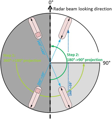
4. AIS-ship-relative-heading: The heading of the ship relative to the radar beam looking direction given by the AIS message. The heading is projected from 360° down to 90° (see Figure 3 for explanation).

5. SAR-ship-length: The length of the ship derived from the SAR signature (Tings, Bentes, and Lehner 2015).

6. SAR-ship-width: The width of the ship derived from the SAR signature (Tings, Bentes, and Lehner 2015).

7. SAR-ship-relative-heading: The heading of the ship relative to the radar beam looking direction derived from the SAR signature (Tings, Bentes, and Lehner 2015). The heading is projected from 360° down to 90° (see Figure 3 for explanation).

8. AIS-ship-velocity: The speed of the ship in knots given by the AIS message.

9. SAR-wind-speed: The wind speed in m s⁻¹ is estimated from the roughness of the sea surface in the SAR image. For TerraSAR-X, the XMOD-2 (Li and Lehner 2013; Jacobsen et al. 2015) and, for Sentinel-1 and RADARSAT-2, the CMOD-5N (Monaldo et al. 2016) geophysical model function is applied.

10. SAR-significant-wave-height: The wave height in m is estimated from sea surface features in the SAR images. For TerraSAR-X, the XWAVE (Bruck and Lehner 2013) and, for Sentinel-1, the CWAVE (Li et al. 2010) empirical model function is applied. For RADARSAT-2, a method for estimating the significant wave height is not available.

Figure 2. Plot of absolute correlation coefficients (Pearson product–moment correlation coefficients) of each parameter with the wake visibility calculated for the X1-MIX (dark green), X1-HH (green), X1-VV (light green), C1-VV (red), and C2-HH (blue) data set.

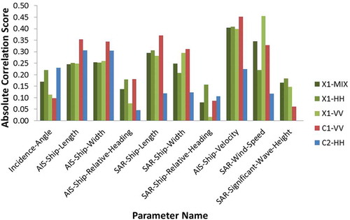
Figure 3. Projection of ship heading down to an interval of 0°–90° relative to the radar beam looking direction (dashed black arrow). The light green arrow visualizes the first projection from 360° to 180°, and the dark green arrow visualizes the second projection from 180° to 90°. The blue arrows present an example projection for one ship heading.

As the parameters AIS-ship-length, AIS-ship-width, SAR-ship-length, and SAR-ship-width represent similar ship features and are therefore almost redundant, the three parameters with lowermost correlation are discarded (i.e. AIS-ship-length, AIS-ship-width, and SAR-ship-width). Also, AIS-ship-relative-heading and SAR-ship-relative-heading are redundant and AIS-ship-relative-heading is discarded because the AIS-independent parameters are preferred in the following analyses. This means six parameters are selected for consideration in the detectability model.

1. Incidence-angle

2. SAR-ship-length

3. SAR-ship-relative-heading

4. AIS-ship-velocity

5. SAR-wind-speed

6. SAR-significant-wave-height

3. Building of detectability models using L2-regularized logistic regression

Building a detectability model is broken down to the training of a binary classifier using the parameters in Figure 2 as feature vectors and the two class labels ‘not detectable’ and ‘detectable.’ The L2-regularized Logistic Regression classifier is explained in Lin, Weng, and Keerthi (2008) and Fan et al. (2008). This classifier has been chosen because it provides linear separating hyperplanes, which are useful for interpreting the detectability model qualitatively. Other classifiers with this capability, e.g. support vector machines, are not able to calculate probabilities for class affiliation (Wu, Lin, and Weng 2004). However, the probability of belonging to the class ‘detectable’ is used here to express the detectability score. Further, the applied training data sets are small and the selection of this less complex model is also justified to prevent possible overfitting. The training data sets are non-sparse and only the selected relevant features are included. Thus, L2 regularization has been applied (Donoho and Huo 2001). As already stated in Lin, Weng, and Keerthi (2008), the classifier training corresponds to a minimization task,

(1) $\mathrm{m}\mathrm{i}{\mathrm{n}}_{\mathit{w}}\mathrm{f}\left(\mathit{w}\right)\equiv \frac{1}{2}{\mathit{w}}^{\mathrm{T}}\mathit{w}+C\sum _{i=1}^N\mathrm{l}\mathrm{o}\mathrm{g}\left(1+{\mathrm{e}}^{-y_i{\mathit{w}}^{\mathrm{T}}{x}_i}\right)$(1)

Here, $C$ is the cost parameter and set to $C=1$, $N$ defines the number of training samples, $x_i$ is the training instances, and $y_i\in \left\{1,-1\right\}$ is the class label with index $i$. $w$ describes the set of weights, which are optimized during the training process. The penalty parameter $C=1$ was determined by 10-fold cross-validation (Kohavi 1995) but identified to have almost no effect on the classification accuracy.

The classifier can be trained with an arbitrary number of parameters. If the number of highly correlated parameters is large, the L1 regularization should then be applied instead of L2 regularization (Donoho and Huo 2001). Nevertheless, in the above listing of the six selected parameters, redundant parameters had already been removed. In order to obtain a separating hyperplane, which is qualitatively interpretable in the 3D space, only three parameters out of the six parameters are used as features for building the classification models.

4. Qualitative analysis

After manual inspection and filtering of unclear wake samples as described in Section 2, the analysed data set contains only wakes that are visible over several hundreds of metres in length and a few tens in width. The resolution of the TerraSAR-X Stripmap and Spotlight images varies between 3.10 and 11.8 m in range and azimuth direction, respectively (pixel spacing between 1.50 and 5.50 m per pixel). The RADARSAT-2 Fine images have a resolution of 10.40 m in range and 6.80–7.70 m in azimuth direction (pixel spacing always equal to 6.25 m per pixel). All Sentinel-1 IW images have a resolution of around 20.40 m in range and 21.70 m in azimuth direction (pixel spacing always equal to 10.00 m per pixel). The difference in resolution in relation to the extent of the wake extent is low. Thus, it was not expected that differences in the detectability of wakes arise from the different resolutions.

In a qualitative analysis, wake samples from the same ship with comparable voyage parameters imaged by different sensors under small spatial and temporal deviations were identified. By downscaling the original TerraSAR-X images to RADARSAT-2 pixel spacing and in turn by downscaling the original TerraSAR-X and RADARSAT-2 images to Sentinel-1 pixel spacing, the influence of the different resolutions on the visibility of wakes was investigated.

For the C- and X-band data set available, many samples of moving ships in the X-band have a clear wake signature, while the same moving ship imaged in the C-band, i.e. either by RADARSAT-2 or Sentinel-1, does not show a pronounced wake signature on the sea surface. This behaviour is maintained even when a downscaling procedure has been applied on the X-band images to coincide with both pixel spacings of the C-band data sets. In our opinion, this finding can be explained by a combination of factors: first, the shorter wavelength in the X-band helps in getting a stronger response from the different wake structures; second, the smaller azimuth cut-off wavelength due to the lower altitude orbit of TerraSAR-X compared to the RADARSAT-2 and Sentinel-1 satellites helps in imaging the wave structures inside the wake and also in imaging the Kelvin wakes in case of ship movement in the azimuth direction. We believe the first factor is the most important, and to verify this statement, we will investigate this in the future by using X-band satellite SAR data from the COSMO-SkyMed constellation, which has a similar orbit altitude to RADARSAT-2 and Sentinel-1.

Figure 4 displays an example comparison of a wake sample from the same ship represented by different sensors, different resolutions, and with different local incidence angles at the ship location in the respective image plane. The overall dependency of the incidence angle on the various frequencies is further investigated in Section 5. The wake is clearly visible on the X-band images, but not on the C-band images. This statement is supported by the graphs in Figure 5, where the averaged sigma naught values of the pixels are plotted; these are located at intersections of the wake in the azimuth direction at a distance of 300 m to the wake vortices and with 400 m length as well as 20 m width. These intersections are indicated by red lines in Figure 4. The averaging was conducted over all pixels in the range direction for each row in the intersections. The graphs in Figure 5 are ordered in the same way as the cut-outs in Figure 4. Wake features in these so-called scan curves, as described in Eldhuset (1996), are only recognizable in the plots corresponding to the TerraSAR-X cut-outs.

Figure 4. Images from different sensors downscaled to identical pixel spacing; left (a), (b), and (d) TerraSAR-X (original pixel spacing 2.75 m × 2.75 m), centre (c,e) RADARSAT-2 (original pixel spacing 6.25 m × 6.25 m), and right (f) Sentinel-1 (original pixel spacing 10.00 m × 10.00 m). All images were acquired on 12 June 2015 over the German Bight. The red line indicates the wake intersections displayed in Figure 5.

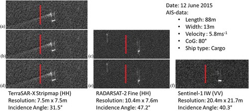
Figure 5. Scan curves of intersections with length of 400 m behind wakes with a distance to the wake vortices of 300 m.

In the X-band data collection, multiple images with dual polarization, i.e. HH- and VV-channel, are available. These images are used for a second qualitative analysis to investigate the difference of wake detectability between HH- and VV-polarized images. Figure 6 presents two examples of wake samples acquired with two polarization channels. The first example was acquired with a low incidence angle and the second example with a high incidence angle. While the sea surface of the low incidence angle example shows hardly any difference, in the VV-channel of the high incidence angle example, the contrast is higher and the wake is better distinguishable from the surrounding background. Although an example with bad wake visibility was chosen deliberately, the wake is visible on both channels. In conclusion, wakes were expected to be better visible on VV-polarized images than on HH-polarized images, but the detectability should only be slightly better. However, this statement is not valid in general, but rather the difference in detectability is subject to the setting of the parameters considered. The qualitative analysis in the next section provides more details (consider Figures 8 and 9).

Figure 6. Wake samples acquired with different incidence angles [top (a,b): incidence angle of 29.6°, and bottom (c,d): incidence angle of 44.5°] and two polarization channels [left (a) and (c)): HH-polarization, and right (b,d): VV-polarization].

Figure 7. Data set X1-MIX; Model One; TerraSAR-X high-resolution wake detectability chart based on SAR-wind-speed, AIS-ship-velocity and from left to right 25, 50, and 100 m SAR-ship-length.

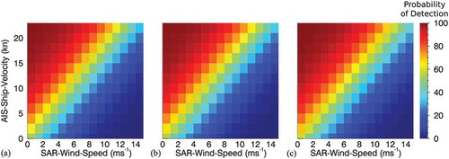
Figure 8. Data set X1-HH; Model One; TerraSAR-X high-resolution HH-polarization wake detectability chart based on SAR-wind-speed, AIS-ship-velocity and from left to right 25, 50, and 100 m SAR-ship-length.

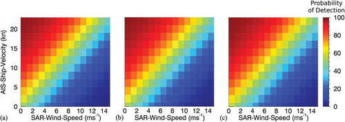
Figure 9. Data set X1-VV; Model One; TerraSAR-X high-resolution VV-polarization wake detectability chart based on SAR-wind-speed, AIS-ship-velocity and from left to right 25, 50, and 100 m SAR-ship-length.

5. Quantitative analysis based on 2D detectability charts

For each training data set, three models were built. Model One is based on the three parameters approaching the highest absolute correlation coefficients based on the X1-MIX data set, i.e. SAR-wind-speed, AIS-vessel-velocity, and SAR-ship-length. In order to have comparable models for all data sets, the correlation coefficients of the other data sets were not considered and the TerraSAR-X data set was the most extensive one. Model Two and Model Three were built only with the parameters that are extractable from SAR images without AIS augmentation. For Model Two, the parameters SAR-wind-speed, SAR-significant-wave-height, and SAR-ship-length are used. These SAR-based parameters are related to environmental conditions. As SAR-significant-wave-height could only be derived for TerraSAR-X and Sentinel-1 images, Model Two is not available for the C2-HH data set. Model Three is based on the parameters SAR-relative-heading, incidence-angle, and SAR-ship-length. These are the remaining parameters with low absolute correlation coefficients based on the X1-MIX data set. The SAR-ship-length is used in all models because it is the SAR-based parameter with the highest correlation coefficient averaged over all data sets. Also, the resulting detectability charts are more easily comparable when based on the same parameter in the third dimension. Model Two and Model Three would also be appropriate for fully automatic wake detection.

In order to outline the dependency of wake detectability on the various parameters, for each data set and for all three classification models, the 2D detectability charts are derived. By setting a fixed SAR-ship-length in all three models, the third dimension is removed and 2D probability maps can be obtained for an easier interpretation of the wake detectability trend as a function of the two parameters selected. Hence, for each model, three charts are calculated by setting a fixed value of the third dimension SAR-ship-length to 25, 50, and 100 m, respectively. Each chart is created in two steps.

1. Binning the co-domain of

   1. Model One: SAR-wind-speed and AIS-ship-velocity into integer splits,

   2. Model Two: SAR-wind-speed and SAR-significant-wave-height into integer splits, and

   3. Model Three: incidence-angle into integer splits and SAR-ship-relative-heading into 5° splits.

2. Calculating the probability of belonging to class ‘detectable,’ respectively,

   1. Model One: for each combination of SAR-wind-speed and AIS-ship-velocity bins,

   2. Model Two: for each combination of SAR-wind-speed and SAR-significant-wave-height bins, and

   3. Model Three: for each combination of incidence-angle and SAR-ship-relative-heading bins.

Figures 7-11 display the derived detectability charts for Model One, Figures 12-15 for Model Two, and Figures 16-20 for Model Three.

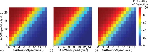
Figure 10. Data set C1-VV; Model One; Sentinel-1 medium-resolution VV-polarization wake detectability chart based on SAR-wind-speed, AIS-ship-velocity and from left to right 25, 50, and 100 m SAR-ship-length.

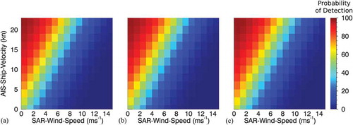
Figure 11. Data set C2-HH; Model One; RADARSAT-2 high-resolution VV-polarization wake detectability chart based on SAR-wind-speed, AIS-ship-velocity and from left to right 25, 50, and 100 m SAR-ship-length.

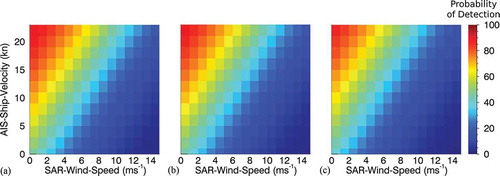
Figure 12. Data set X1-MIX; Model Two; TerraSAR-X high-resolution wake detectability chart based on SAR-wind-speed, SAR-significant-wave-height and from left to right 25, 50, and 100 m SAR-ship-length.

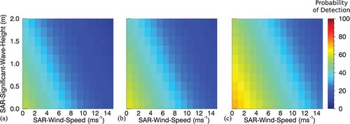
Figure 13. Data set X1-HH; Model Two; TerraSAR-X high-resolution HH-polarization wake detectability chart based on SAR-wind-speed, SAR-significant-wave-height and from left to right 25, 50, and 100 m SAR-ship-length.

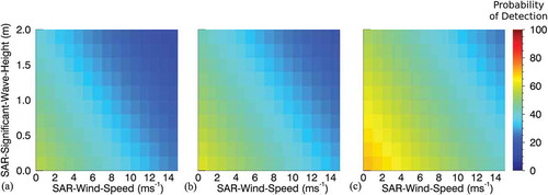
Figure 14. Data set X1-VV; Model Two; TerraSAR-X high-resolution VV-polarization wake detectability chart based on SAR-wind-speed, SAR-significant-wave-height and from left to right 25, 50, and 100 m SAR-ship-length.

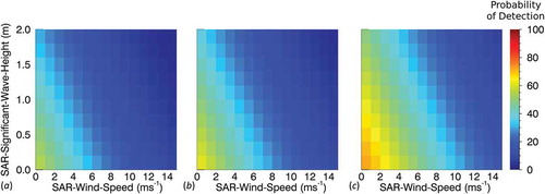
Figure 15. Data set C1-VV; Model Two; Sentinel-1 medium resolution VV-polarization wake detectability chart based on SAR-wind-speed, SAR-significant-wave-height and from left to right 25, 50, and 100 m SAR-ship-length.

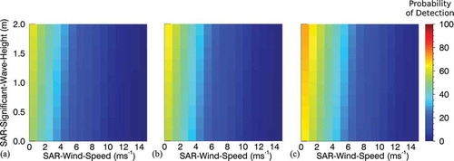
Figure 16. Data set X1-MIX; Model Three; TerraSAR-X high-resolution wake detectability chart based on incidence-angle, SAR-ship-relative-heading and from left to right 25, 50, and 100 m SAR-ship-length.

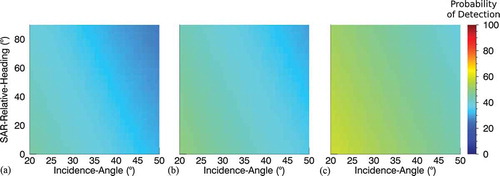
Figure 17. Data set X1-HH; Model Three; TerraSAR-X high-resolution HH-polarization wake detectability chart based on incidence-angle, SAR-ship-relative-heading and from left to right 25, 50, and 100 m SAR-ship-length.

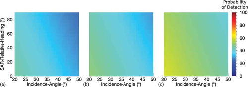
Figure 18. Data set X1-VV; Model Three; TerraSAR-X high-resolution VV-polarization wake detectability chart based on incidence-angle, SAR-ship-relative-heading and from left to right 25, 50, and 100 m SAR-ship-length.

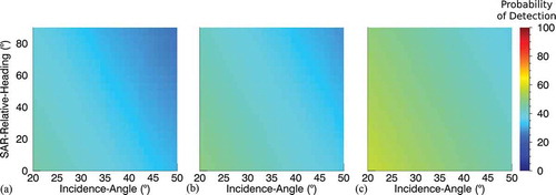
Figure 19. Data set C1-VV; Model Three; Sentinel-1 medium resolution VV-polarization wake detectability chart based on incidence-angle, SAR-ship-relative-heading and from left to right 25, 50, and 100 m SAR-ship-length.

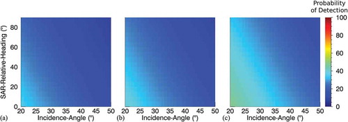
Figure 20. Data set C2-HH; Model Three; RADARSAT-2 high-resolution HH-polarization wake detectability chart based on incidence-angle, SAR-ship-relative-heading and from left to right 25, 50, and 100 m SAR-ship-length.

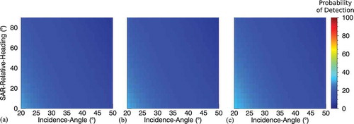
In general, a lower probability of detection of wakes in C-band data sets compared to the X-band data sets is observable. The 2D detectability charts support the following statements about the selected parameters for all SAR missions considered.

1. The lower the incidence angle, the better wakes are detectable.

2. The larger the ship, the better wakes are detectable.

3. Ships moving along the looking direction of the radar beam show wakes which are better detectable, and ships moving along the azimuth direction of the satellite show wakes which are less detectable.

4. The faster the ship movement, the better wakes are detectable.

5. The lower the SAR-derived wind speed, the better wakes are detectable.

For RADARSAT-2, the significant wave height is not available and for Sentinel-1, the charts show slightly contradictory dependencies on the significant wave height. As the method for significant wave height estimation on Sentinel-1 images is still in an experimental state, the corresponding detectability model is discarded. The following statement therefore only holds for TerraSAR-X.

• (6) The lower the SAR-derived significant wave height, the better wakes are detectable.

The magnitude with which the detectability corresponds to the parameters differs not only between the sensors but also between the polarizations, as already indicated by the correlation coefficients in Figure 2. Comparisons between the charts of Figures 8 and 9 as well as Figures 13 and 14 reveal that the detectability of wakes decreases more prominently for higher wind speed conditions in the X1-VV data set than in the X1-HH data set. Figures 8 and 9 also display a more prominent increase of detectability for higher ship velocities in the X1-VV data set than in the X1-HH data set. The same difference in magnitude can also be observed in Figures 10 and 11 between the C1-VV and C2-HH data sets, although the general detectability is lower in the C-band. Comparing only the met-ocean parameters in Figures 13 and 14, the detectability of wakes is significantly lower in the X1-VV than in the X1-HH data set, but the difference is neither pronounced in Figures 8 and 9 nor in Figures 17 and 18. We therefore conclude that, in general, detectability does not differ between HH- and VV-polarization but does depend with differing magnitudes on the selected parameters. By confronting Figures 10 and 11 with Figures 19 and 20, this conclusion is supported, since overall detectability seems higher in the C2-VV data set than in the C1-HH data set in Figures 10 and 11, in contrast to Figures 19 and 20, which show lower detectability in the C2-VV data set than in C1-HH data set.

6. Discussion and outlook

A detectability model based on L2-regularized logistic regression trained with TerraSAR-X (X1-MIX), TerraSAR-X HH-polarization (X1-HH), TerraSAR-X VV-polarization (X1-VV), Sentinel-1 VV-polarization (C1-VV), and RADARSAT-2 HH-polarization (C2-HH) data is presented. As the model is linear, linear relationships between the detectability of ship wakes and the parameters describing image acquisition settings, met-ocean conditions, and ship design features are also pronounced.

The results presented are based on models using three dimensions and therefore only considering three parameters at a time. As classification models are arbitrarily scalable to any amount of features, the proposed method for building detectability models for ship wakes is arbitrarily scalable as well. However, the results of such a high-dimensional model are more difficult to visualize, but in the future, the model would be capable of providing useful a-priori information for the automatic detection of ship wakes and the targets themselves.

In future research, non-linear relationships between the parameters should also be investigated by using a more complex non-linear detectability model. Because the respective classification model must only be capable of calculating the probabilities of class affiliation, a large number of possibilities exist. Further, the influence of the satellite orbit altitude and the resulting differences in azimuth cut-off effect should be evaluated by confrontation of TerraSAR-X with COSMO-SkyMed data.

Besides application of the model for the improvement of wake detection systems, the model could also be reversed to determine ship parameters. For the case that a wake has already been detected in a SAR image and all parameters except one are known, the model can be applied backwards to estimate the minimum value of this parameter. For example, it would be possible to derive the minimum speed a vessel must have under certain conditions to ensure that its wake is visible.

Disclosure statement

No potential conflict of interest was reported by the authors.

References

- Bruck, M., and S. Lehner. 2013. “Coastal Wave Field Extraction Using TerraSAR-X Data.” Journal of Applied Remote Sensing 7 (1): 1–19. doi:10.1117/1.JRS.7.073694.
- Copeland, A. C., G. Ravichandran, and M. M. Trivedi. 1995. “Localized Radon Transform-Based Detection of Ship Wakes in SAR Images.” IEEE Transactions on Geoscience and Remote Sensing 33 (1): 35–45. doi:10.1109/36.368224.
- Crisp, D. J. 2004. The State-of-The-Art in Ship Detection in Synthetic Aperture Radar Imagery. Edinburgh: DSTO Information Sciences Laboratory.
- Donoho, D. L., and X. Huo. 2001. “Uncertainty Principles and Ideal Atomic Decomposition.” IEEE Transactions on Information Theory 47 (7): 2845–2862. doi:10.1109/18.959265.
- Eldhuset, K. 1996. “An Automatic Ship and Ship Wake Detection System for Spaceborne SAR Images in Coastal Regions.” IEEE Transactions on Geoscience and Remote Sensing 34 (4): 1010–1019. doi:10.1109/36.508418.
- ESA. 2017. “Copernicus Observing the Earth” ESA. Accessed 21 September 2017. http://maritimesurveillance.security-copernicus.eu/
- Fan, R.-E., K.-W. Chang, C.-J. Hsieh, X.-R. Wang, and C.-J. Lin. 2008. “LIBLINEAR: A Library for Large Linear Classification.” Journal of Machine Learning Research 9: 1871–1874.
- Graziano, M. D., M. D’Errico, and G. Rufino. 2016a. “Ship Heading and Velocity Analysis by Wake Detection in SAR Images.” Acta Astronautica 128: 72–82. doi:10.1016/j.actaastro.2016.07.001.
- Graziano, M. D., M. D’Errico, and G. Rufino. 2016b. “Wake Component Detection in X-Band SAR Images for Ship Heading and Velocity Estimation.” Remote Sensing 6 (8): 1–15. doi:10.3390/rs8060498.
- Jacobsen, S., S. Lehner, J. Hieronimus, J. Schneemann, and K. Michael. 2015. “Joint Offshore Wind Field Monitoring with Spaceborne SAR and Platform-Based Doppler LiDAR Measurements.” International Archives of the Photogrammetry, Remote Sensing and Spatial Information Sciences XL-7/W3: 959–966. doi:10.5194/isprsarchives-XL-7-W3-959-2015.
- Joint Research Centre. 2017. “Blue Hub – Transform Data into Knowledge.” European Comission. Accessed 24 January 2017. https://bluehub.jrc.ec.europa.eu/
- Kohavi, R. 1995. “A Study of Cross-Validation and Bootstrap for Accuracy Estimation and Model Selection.” Proceedings of the Fourteenth International Joint Conference on Artificial Intelligence 2: 1137–1143.
- Li, X-M., and Lehner S. 2013. “Algorithm for Sea Surface Wind Retrieval from TerraSAR-X and TanDEM-X Data.” IEEE Transactions on Geoscience and Remote Sensing 2928–2939. doi:10.1109/TGRS.2013.2267780.
- Li, X., T. Koenig, J. Schulz-Stellenfleth, and S. Lehner. 2010. “Validation and Intercomparison of Ocean Wave Spectra Inversion Schemes Using ASAR Wave Mode Data.” International Journal of Remote Sensing 31 (17): 4969–4993. doi:10.1080/01431161.2010.485222.
- Lin, C.-J., R. C. Weng, and S.S Keerthi. 2008. “Trust Region Newton Method for Large-Scale Logistic Regression.” Journal of Machine Learning Research 627–650. doi:10.1145/1273496.1273567.
- Meta, A., J. Mittermayer, P. Prats, R. Scheiber, and U. Steinbrecher. 2009. “TOPS Imaging with TerraSAR-X: Mode Design and Performance Analysis.” IEEE Transactions on Geoscience and Remote Sensing 48 (2): 759–769. doi:10.1109/TGRS.2009.2026743.
- Monaldo, F., C. Jackson, L. Xiaofeng, and W. G. Pichel. 2016. “Preliminary Evaluation of Sentinel-1A Wind Speed Retrievals.” IEEE Journal of Selected Topics in Applied Earth Observations and Remote Sensing 9 (6): 2638–2642. doi:10.1109/JSTARS.2015.2504324.
- Pearson, K. 1895. “Notes on Regression and Inheritance in the Case of Two Parents.” Proceedings of the Royal Society of London 58: 240–242. doi:10.1098/rspl.1895.0041.
- Pichel, W. G., P. Clemente-Colón, C. C. Wackerman, and K. S. Friedman. 2004. “Ship and Wake Detection.” In Chap. 12 in Synthetic Aperture Radar Marine User’s Manual, edited by C. R. Jackson and J. R. Apel, 277–303. Washington, DC: U.S. Department of Commerce.
- Soloviev, A., M. Gilman, K. Young, S. Brusch, and S. Lehner. 2010. “Sonar Measurements in Ship Wakes Simultaneous with TerraSAR-X Overpasses.” IEEE Transactions on Geoscience and Remote Sensing 48 (2): 841–851. doi:10.1109/TGRS.2009.2032053.
- Tings, B., C. Bentes, and S. Lehner. 2015. “Dynamically Adapted Ship Parameter Estimation Using TerraSAR-X Images.” International Journal of Remote Sensing 37 (9): 1990–2015. doi:10.1080/01431161.2015.1071898.
- Velotto, D., C. Bentes, B. Tings, and S. Lehner. 2016. “First Comparison of Sentinel-1 and TerraSAR-X Data in the Framework of Maritime Targets Detection: South Italy Case.” IEEE Journal of Oceanic Engineering 41 (4): 993–1006. doi:10.1109/JOE.2016.2520216.
- Wu, T., C.-J. Lin, and R. C. Weng. 2004. “Probability Estimates for Multi-Class Classification by Pairwise Coupling.” Journal of Machine Learning 5: 975–1005.
- Zilmann, G., A. Zapolski, and M. Marom. 2014. “On Detectability of a Ship’s Kelvin Wake in Simulated SAR Images of Rough Sea Surface.” IEEE Transactions on Geoscience and Rome Sensing 53 (2): 609–619. doi:10.1109/TGRS.2014.2326519.