Estimating fractional cover of plant functional types in African savannah from harmonic analysis of MODIS time-series data

ABSTRACT

Assessments of tree/grass fractional cover in savannahs using remote sensing are challenging due to the heterogeneous mixture of the two plant functional types. Time-series decomposition models can be used to characterize vegetation phenology from satellite data, but have rarely been used for attributing phenological signal components to different plant functional types. Here, tree/grass dynamics are assessed in savannah ecosystems using time-series decomposition of 14 years of Moderate Resolution Imaging Spectroradiometer (MODIS) normalized difference vegetation index data acquired from 2002 to 2015. The decomposition method uses harmonic analysis and tests the individual harmonic terms for statistical significance. Field data of fractional cover of trees and grasses were collected for 28 plots in Kruger National Park, South Africa. Matching MODIS pixels were analysed for their tree/grass phenological signals. Tree/grass annual and interannual variability were then assessed based on the harmonic models. In most harmonic cycles, grass-dominated sites had higher amplitudes than tree-dominated sites, while the tree green-up started earlier than grasses, before the start of the wet season. While changes in tree phenology are gradual, grasses present higher variability over time. Tree cover showed a significant correlation with the amplitude (r (correlation coefficient) = −0.59, p = 0.001) and phase of the first harmonic term (r = −0.73, p = 0.0001) and the number of cycles of the second harmonic term (r = 0. 56, p = 0.002). Grass cover was also significantly correlated with the amplitude (r = 0. 51, p = 0.005) and phase of the first harmonic term (r = 0.55, p = 0.002) and the number of cycles of the second harmonic term (r = −0.52, p = 0.005). The positive correlation of grass cover with phase and negative correlation with number of cycles is indicating a late greening period and higher variability, respectively. Tree cover estimated from the phase of the strongest harmonic term showed a positive correlation with field-measured tree cover (R² (coefficient of determination) = 0.55, p < 0.01, slope = 0.93, root mean square error = 13.26%). The estimated tree cover also had a strong correlation with the woody cover map (r = 0.78, p < 0.01) produced by Bucini. The results show that MODIS time-series data can be used to estimate the fractional tree cover in heterogeneous savannahs from the phase of the plant functional type’s phenological behaviour. This study shows that harmonic analysis is able to discriminate between fractional cover by trees and grasses in savannahs. The quantitative analysis of tree/grass phenology from satellite time-series data enables a better understanding of the dynamics of the tree/grass competition and coexistence.

KEYWORDS:

• NDVI
• harmonic analysis
• decomposition
• vegetation phenology
• savannah
• tree cover
• grass cover

1. Introduction

Monitoring long-term changes in the composition of tree/grass cover in savannahs is required for an assessment of the ecosystem response to a changing climate (Yang, Weisberg, and Bristow 2012; Cleland et al. 2007). Remote-sensing methods are currently being developed to enable the exploration and modelling of the role of vegetation dynamics in ecosystems processes, biosphere–atmosphere exchange, and carbon cycle processes (e.g. carbon sequestration). This requires differentiation of plant functional types (PFTs). Large-scale information on the PFT composition of a landscape can reveal ecological processes leading to vegetation fluctuation and succession to assess ecosystem vulnerability to environmental change (Lu et al. 2003; Smith et al. 2014a; Smith et al. 2014b).

Tree/grass co-existence and their interactions with environmental factors have been described by several authors (Hill and Hanan 2010; Accatino et al. 2010; Scholes and Archer 1997). The influence of human activities (agriculture, wood collection) and physical factors such as rainfall, fire, geology, and herbivory on the tree/grass mixture in savannahs has been extensively studied (Sankaran, Ratnam, and Hanan 2008; Bond and Keeley 2005; Smit et al. 2010; Asner et al. 2009). Previous studies have conceptualized the distribution of vegetation in savannah as a function of soil, climatic gradient, and human activities (Foody 2003; Chamaille-Jammes, Fritz, and Murindagomo 2006; Chamaille-Jammes and Fritz 2009).

To this date, the full potential of remote sensing in mixed tree/grass plant communities using time-series analysis has not yet been realized. Challenges lie in detecting differences in tree/grass cover, structure, physiology, phenology, and seasonality. Because the signals from PFTs are mixed within pixels in medium-resolution satellite images, these components have to be unmixed (Hill et al. 2011; Hill and Hanan 2010). PFT mapping from time-series decomposition of satellite such as Moderate Resolution Imaging Spectroradiometer (MODIS) or Advanced Very High Resolution Radiometer (AVHRR) adds immense value because of the availability of long-term satellite data archives (Lu et al. 2003; Archibald and Scholes 2007).

Few studies have tried to discriminate the woody and herbaceous signals from satellite time-series data (Roderick, Noble, and Cridland 1999; Lu et al. 2003; Archibald and Scholes 2007). Finding suitable methods for analysing multi-temporal satellite data is one of the most significant challenges facing remote sensing (Martínez and Gilabert 2009). The availability of remotely sensed time-series satellite data covering more than three decades provides a vast data resource for vegetation characterization and measurement. Remotely sensed time-series data are relevant for studying plant phenology because of their consistency and repeatability at a large spatial scale (Verbesselt et al. 2010). Despite their limitations due to the phenology itself, interannual climate variability, disturbance, signal contamination, and sensor conditions, remote-sensing studies on the application of phenology in ecology, agriculture, modelling climate, and human-induced changes have been widely published. The analysis of the normalized difference vegetation index (NDVI), fraction of absorbed photosynthetically active radiation (fAPAR), and leaf area index using time-series satellite data from the AVHRR, MODIS, and Landsat for detecting vegetation phenology has been applied to the estimation of net primary productivity (Tucker and Sellers 1986; Reed et al. 1994), fire risk assessment (Hernandez-Leal, Arbelo, and Gonzalez-Calvo 2006), crop-type discrimination (Mingwei et al. 2008), biosphere/climate feedbacks (Balzter et al. 2007), and vegetation dynamics (Martínez and Gilabert 2009; Verbesselt et al. 2010).

Fractional cover of trees/grasses in African savannahs has been separated by some authors using signal decomposition methods (Lu et al. 2003; Archibald and Scholes 2007). Information based on the biochemical and biophysical properties of woody and herbaceous components can be used to discriminate the two vegetation components using spectral signatures (Hill et al. 2011; Cho et al. 2012). Tree and grass signal separation is based on the assumption that trees and grasses exhibit different biological characteristics in their life forms, which can be separated using phenological metrics assessed through moving-average method (Archibald and Scholes 2007). In savannahs, trees green up before grasses because their deeper roots rely less on water from rainfall (Whitecross, Witkowski, and Archibald 2017a). In spite of the fact that the moving-average method usually maintains the area and mean position of the seasonal peak in a time series of satellite data (Eklundha and Jönssonb 2012), one cannot assume that the moving average captures all phenology metrics including those due to noise, fire, and land degradation. There are also no standard criteria for choosing the delay time in the moving window, which consequently affects the degree of changes being observed in the data (de Beurs and Henebry 2010; Verbesselt et al. 2010).

Lu et al. (2003) developed a model that decomposes tree/grass phenology signals from AVHRR data considering vegetation biophysical characteristics and noise reduction. The model is an extension of the Seasonal-Trend Decomposition based on the Loess algorithm (Cleveland et al. 1990). Although the model retrieves periodic information on regional and global vegetation, one limitation is the selection of the threshold to determine low- and high-varying components of woody and herbaceous cover. The tendency for over- or underestimation of these components is very high and can result in false separation of the vegetation index components (Lu et al. 2003).

As an alternative approach, harmonic analysis is based on the Fourier transform and is one of the most reliable techniques for land-cover discrimination from decoupled vegetation phenological signals (Andres, Salas, and Skole 1994; Kostadinov et al. 2017). Harmonic analysis enables a phenological time series to be expressed as a sum of cosine waves and an additive term. Each individual wave is called a harmonic term and is characterized by its amplitude (height of the maximum), frequency (number of cycles), and phase (delay from time zero). Previous studies have used this method successfully to characterize seasonal changes in natural land-cover and land-use types (Jakubauskas, Legates, and Kastens 2001; Jakubauskas, Legates, and Kastens 2002; Canisius, Turral, and Molden 2007; Westra and De Wulf 2007). Jung and Chang (2015) assessed land-cover change using harmonic analysis. Muñoz Peña and Navarro (2016) applied harmonic analysis to study deforestation in Peru’s Tahuamanu province from 2001 to 2011. Moody and Johnson (2001) applied discrete Fourier analysis to derive a mean-phase-amplitude space to separate six vegetation types from different geographical regions by classifying AVHRR data. Validation results indicated that grassland had the highest accuracy (77%) and the most common confusion in their classification accuracy was between grassland and savannah (23%). This was partly due to mixed pixels being influenced by annual grass understorey variations. Mapping fractional tree/grass cover as a continuous variable is needed in African savannahs as these landscapes are dominated by gradual transitions between open and closed shrub and grasslands rather than by distinct land-cover classes and boundaries (Gessner, Ursula, Christopher Conrad, Christian Huttich, Manfred Keil, Michael Schmidt, Matthias Schramm, and Stefan Dech 2008). In addition, most previous studies on harmonic analysis do not provide analytical error structure of the estimated harmonics (Jakubauskas and David 2000; Moody and Johnson 2001).

The use of confidence intervals in time series is important as they can distinguish a statistically rare event from events within the expected range of variability at a given level of confidence (White and Nemani 2006). White and Nemani (2006) presented a statistical measure of uncertainty using confidence intervals for real-time monitoring and short-time forecasting of land surface phenology (LSP). They analysed the phenological behaviour of a group of pixels without fitting. While the uncertainty of LSP estimation can be expressed through a confidence interval, in general, the uncertainty of the metrics of LSP from harmonic analysis has not been adequately addressed in remote-sensing studies (de Beurs and Henebry 2010; Moody and Johnson 2001). Statistical techniques to estimate confidence intervals are necessary (Bloomfield 2004).

This study aimed to use harmonic analysis to satellite time-series data on tree/grass phenology by estimating statistically significant harmonic terms using the Hartley test and correcting for multiple testing with the Bonferroni method. We estimate the seasonal cycle, amplitude, and phase derived from the annual frequency over the entire time series (14 year MODIS NDVI). The study presents a novel remote-sensing approach that can in principle be applied to the assessment of tree/grass phenology in savannah sites worldwide.

2. Materials and methods

2.1. Study area

Kruger National Park (KNP) is one of the largest national parks in Africa. It is approximately 2 million hectares in size and extends 380 km from north to south and 60 km from east to west. Its elevation ranges from 260 to 839 m above mean sea level. The average annual rainfall ranges from 440 mm in the north to 750 mm in the south. The park has large perennial rivers as well as seasonally flooded dryland river channels (Figure 1). Geologically, the area is divided into two main zones. The western part is dominated by granite and the eastern part by basaltic bedrocks. Therefore, a strong influence of geological structures on soil types and plant species distribution is observable in the park (Eckhardt, Van Wilgen, and Biggs 2000; Archibald and Scholes 2007; Khalefa et al. 2013). The distribution of vegetation types is associated with climate, geology, and topography of the area.

Figure 1. Location of the study area of Kruger National Park in South Africa and its main river courses overlaid on high-resolution Google imagery. The blue circles indicate the field plot locations collected in 2015.

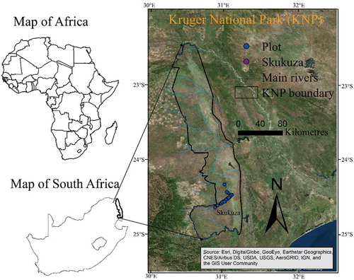
KNP is home to more than 1900 tree and grass species (Eckhardt, Van Wilgen, and Biggs 2000). The status of each PFT has been a focus of savannah ecology for many decades. The park has 20 vegetation communities (e.g. Skukuza thickets, open trees, dense trees, and bush savannah) based on a floristic classification (Eckhardt, Van Wilgen, and Biggs 2000; Archibald and Scholes 2007; Khalefa et al. 2013). The dominant tree species in the southern part include Combretum apiculatum, Acacia nigrescens, Spirostachys africana, Combretum hereroense, Sclerocarya birrea, Terminalia sericea, Combretum zeyheri, etc. The drier northern part is dominated by mopane savannah. Grass species include Aristida congesta spp., Digitaria eriantha, Erasiantha, Urochloa mosambicensis, Themeda triandra, and Panicum coloratum (Eckhardt, Van Wilgen, and Biggs 2000; Archibald and Scholes 2007; Khalefa et al. 2013).

The study area was chosen because it hosts a large diversity of vegetation types (from floristic and structural perspectives, e.g. large range of tree cover 20–80%) at the MODIS pixel size of 250 m. The distribution of vegetation types is associated with climate and topography of the area. Harmonic analysis is more applicable in a diverse area with varied species composition and large variations of environmental conditions (Moody and Johnson 2001).

2.2. MODIS NDVI time-series data

MODIS NDVI data (MOD13Q1) were obtained from the National Aeronautics and Space Administration (NASA) (http://reverb.echo.nasa.gov/reverb). MOD13Q1 is a gridded level 3 product provided at 250 m spatial resolution every 16 days. We used the quality-assured product that is already atmospherically corrected for bi-directional reflectance function effects to reduce the effects of water, clouds, and cloud shadows, etc. This data product has been used widely for retrieving vegetation information such as vegetation structure and annual net primary productivity dynamics in grassland–shrub land areas (Moreno-de Las et al. 2015), tree cover change (Gill et al. 2009), and tree–grass separation of green-up dates (Archibald and Scholes 2007). Furthermore, Jung and Chang (2015) assessed land-cover change from harmonic analysis using NDVI data. Muñoz Peña and Navarro (2016) assessed the spatio-temporal variability of NDVI to study deforestation using harmonic analysis. NDVI has also been used to examine the relationship between vegetation productivity and rainfall distribution along environmental gradients (Foody 2003; Chamaille-Jammes and Fritz 2009). NDVI is better suited to sparse vegetation such as savannahs (due to low biomass) as well as due to their heterogeneity at MODIS spatial resolution of 250 m, which can capture not only live vegetation phenology (patches of grass, shrubs, and trees) but also litter and soil backgrounds (Jung and Chang (2015)).

2.3. Bucini woody cover map

The Bucini woody cover map was provided by the Scientific Services (GIS unit) of South African National Parks. The woody cover map was produced for KNP at 90 m spatial resolution by calibrating remote-sensing data with field measurements (Bucini et al. 2009; Bucini et al. 2010). Landsat ETM+ bands (blue, green, and red (0.45–0.69 µm), infrared (0.77–0.90 µm), shortwave infrared (1.5–1.75 µm), and the shortwave infrared 2 (2.08–2.35 µm)) acquired between 2000 and 2001 and JERS-1 synthetic aperture radar (SAR) scenes (L-band, HH polarization) acquired between 1995 and 1996 were used to build multiple regression models with field woody cover data. The Landsat scenes were acquired during the beginning of the dry season to maximize the discrimination of green woody canopies from the senesced grass layer. The best predictive model included the JERS-1 backscatter and Landsat band 2 (green), and was used to predict woody cover for KNP. The validation of the woody cover showed an R² = 061, residual error = 0.89 and p < 0.0001 (Bucini et al. 2009). The map was resampled to 250 m through bilinear interpolation to match the MODIS data sets.

2.4. Field data

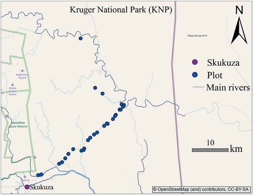
A field campaign was carried out in March 2015 towards the end of the wet season when the vegetation photosynthetic activity was still high (Archibald and Scholes 2007). Fractional vegetation cover (FVC) of four structural vegetation types was estimated visually within 25 plots (trees > 6 m, tree and shrubs 1–6 m, forbs and grasses) along the road from Skukuza to Tshokwane, following the visual estimation procedure proposed by Law et al. (2008). Three additional plots were added based on visual interpretation of Google Earth images to incorporate areas with denser tree cover than what was sampled in the field.

Trees and shrubs were merged to a single PFT group to represent overall woody cover, while forbs and grasses were merged to describe overall grass cover. Figure 2 shows the field plot locations. The field plots were established at least 50 m away from the road to avoid proximity effects on vegetation composition (Smit and Asner 2012). Considering the MODIS pixel size of 250 m each plot was chosen as a 200 m × 200 m square along the 25 km long transect. A distance of at least 1 km was maintained between subsequent plots to capture landscape variability. The procedure starts by establishing a plot boundary, then walking through the plot. It should be noted however that no subplot measurement was done during the field data collection process due to nature of the study area (Riemann et al. 2016; Mairota et al. 2015). Previous studies have highlighted the difficulty of relating field information to image data at comparable scale due to product mismatch and insufficient field data if the plots are smaller than 0.1 km² (Gill et al. 2009).

Figure 2. Relationship between the field data on per cent tree cover and the lidar/SAR tree cover estimate.

The plots spanned different vegetation types, geological conditions, and soil types and cover a gradient of tree/grass mixtures that is very distinct in terms of structure, type, density, and distribution. The plots are in the southern part of KNP where the average annual rainfall is 750 mm. The vegetation in these plot locations, as in many other parts of KNP, also had a history of fire events, drought, and destruction due present of animals such as the elephant (Asner et al. 2009; Bucini et al. 2010; Smit and Asner 2012). Tree species found in the plots include Acacia gradicortuna (e.g. plots 17, 25, and 19), Combretum (zeyheri/apiculatum) (e.g. plots 14, 10, and 6), A. nigrescens (e.g. plot 12), Dichrostachys cinerea, S. birrea, T. sericea (e.g. plot 28), Euclea divinorum (e.g. plot 11), C. hereroense (e.g. plot 19), Albizia harveyi (e.g. plot 9), T. sericea (e.g. plot 22), etc. Grass species include A. congesta spp., D. eriantha, Erasiantha spp., U. mosambicensis, T. triandra, and Panicum coloratum.

A recent study compared four methods of estimating tree canopy cover (Riemann et al. 2016). These methods include stem-mapped canopy cover (SMCC), which is derived directly from ground inventory data using modelled relationships between tree diameter at breast height and crown diameter for each tree species, the field-collected per cent canopy cover (FCC) derived through ocular estimates, photo-interpreted per cent canopy cover data (PCC) (PCC collected from leaf-on, 1 m resolution, digital colour-infrared National Agriculture Imagery Program imagery) and geographic-object-based image analysis approach that uses both high-resolution imagery and leaf-off lidar data. Root mean square error (RMSE) and coefficient of agreement (AC) were used to compare the accuracy of the methods. FCC (ocular-based method) show high agreement with PCC (AC: 0.73, RMSE = 16), GCC (AC = 0.7, 23%), and SMCC (AC = 0.78, RMSE = 14%). The FCC was also evaluated based on quality assurance data, which is collected on 4% of the plots nationwide of the original plots (revisit and re-inventory by a separate crew and all variables are re-measured). The results indicate better agreement (AC = 0.92, RMSE = 7.4) than what was observed in all the previous methods. In this study, the field-estimated tree cover was compared with a high-resolution tree cover estimated from lidar and SAR data by Naidoo et al. (2015) (Figure 3). The lidar data were acquired in April 2008 (end of wet season) when woody plants were leaf-on, and the SAR images in July–August 2008 (dry season, leaf-off) to avoid soil moisture effects on the radar signal (Mathieu et al. 2013). Validation of the SAR map with independent lidar data produced an R² = 0.8 and RMSE = 7.7%. Detail explanation on lidar/SAR estimate of tree cover can be found in Naidoo et al. (2015). The field data on per cent tree cover strongly correlated with the lidar/SAR estimate (r = 0.67, p < 0.001, Figure 3). Ocular estimates together with satellite data have promise for large area estimation of tree cover (Riemann et al. 2016).

Figure 3. Map of the study sites along the Skukuza/Tshokwane road, showing field plot locations.

2.5. Methods

2.5.1. Harmonic analysis of NDVI

Over each field plot location, the phenology features were extracted from the MODIS 16-day composite NDVI time-series data from 2004 to 2014. A discrete Fourier analysis was applied to decompose the time series into harmonic terms that characterize phenology features of woody and herbaceous vegetation. A time series can be represented as the sum of cosine waves where each wave is represented by its amplitude and phase (Jakubauskas, Legates, and Kastens 2001):

(1) $f\left(t\right)=\overline{f\left(t\right)}+\sum _{n=1}^{L/2}(A_n\mathrm{c}\mathrm{o}\mathrm{s}\frac{2\pi nt}{L}-{\mathrm{\varnothing }}_n)$(1)

where $f\left(t\right)$ stands for the NDVI for a given composite and $\overline{f\left(t\right)}$is the mean of the $f\left(t\right)$; A_n denotes the amplitude A of harmonic term n; ${\mathrm{\varnothing }}_n$ represents the phase of the nth harmonic term; and L is the number of observations in the time series (de Beurs and Henebry 2010).

The NDVI pixel time-series data covering each field plot were transformed from the time domain into the frequency domain to retrieve a periodogram. For each harmonic term, the frequency, amplitude, and phase were estimated. The harmonic analysis model implements a linear detrending method to remove the gradient from the data. It then identifies the strongest harmonic terms based on their amplitudes and tests for significance using the test by Hartley (1949). An analysis of variance (ANOVA) was used to test the null hypothesis that there are no significant harmonic terms within the time series. Multiple comparisons of the means following ANOVA used the one-tailed Bonferroni/Holm method to control the experiment-wise type I error at 5% for multiple testing (Köhl, Magnussen, and Marchetti 2006).

2.5.2. Variability of amplitude and phase of the harmonic terms

Harmonic analysis was applied to the pixel-wise NDVI time series for each field plot location. All statistically significant harmonic terms were identified. The interannual variability in amplitude and phase for these plots was then assessed. The analysis of six individual plots is presented in Section 3 for illustration. These plots cover parts of the thickets of the Sabie and Crocodile Rivers, where tree species are dominated by C./. sericea woodland, S. birrea, E. divinorum, S. africana, A. nigrescens, and Acacia welwitschii thickets in the Karoo sediments landscape.

The strongest and second strongest harmonic terms allow ecological interpretation (Scharlemann et al. 2008; Moody and Johnson 2001) as they represent the annual and biannual signals, respectively. The first harmonic term (annual signal) can be caused by either PFT while the second harmonic term is more likely to represent the PFT with bimodal (i.e. two peaks per year) phenological characteristics (Moody and Johnson 2001).

Annual rainfall data from four meteorological stations were compared using bar and line plots with the corresponding amplitude values of the second strongest harmonic term and the mean NDVI of the dry season for each year from 2002 to 2015. The stations include Skukuza and Satara (in the south), Pafuri and Mahlengeni (in the north).

2.5.3. Correlation analysis

Pearson correlation coefficients (r) between tree and grass cover measured in the field and the harmonic coefficients (number of cycles, amplitude, and phase) were calculated (α = 0.05).

2.5.4. Calibration and validation of tree cover estimates with phase values using field data

Linear regression was used to estimate per cent tree cover using the phase of the strongest harmonic term. The field data were divided into two independent sets: one half were used for calibration and the other for validation. To assess model performance for tree cover estimated from the phenology, coefficient of determination (R²) and RMSE were calculated.

3. Results

3.1. Time series of PFT per cent cover

NDVI time-series data for selected field plots with different mixtures of FVC of trees and grasses are presented in Figures 4(a–d). These graphs do not clearly represent the FVC of individual PFT except for years with an unusual event. Generally, a distinction can be made between tree- and grass-dominated sites regarding their minimum and maximum NDVI values. Most of the sites dominated by grasses show lower minima and higher maxima (NDVI values 0.1–0.8) than tree-dominated sites (>0.3). The PFTs show interannual variability in NDVI.

Figure 4. Time-series plots of selected field plots with different FVC of the tree and grass PFT: (a) tree-dominated site (plot 28) and grass-dominated site (plot 3), (b) tree-dominated site (plot 25) and grass-dominated site (plot 4), (c) mixed tree/grass site (plots 17 and 24), and (d) mixed tree/grass site (plots 21 and 11).

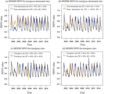
Figures 4(a,b) distinguish between a tree- and a grass-dominated site. The difference between the two is most obvious in the very dry growing season of 2002/2003. In this year, very little grass growth was observed while tree species maintained a relatively high NDVI. Biologically, trees are more resilient to water-constrained conditions than grasses. Trees usually have well-developed roots, which enable them to extract groundwater. They are less dependent on rainfall than the shallow-rooting grasses, which rely on short-lived rainfall (Whitecross, Witkowski, and Archibald 2017b). Trees are also more resistant to fire and can recover more easily after a fire once they have grown to a certain height and escaped the ‘fire trap’. In the NDVI time series, little variation between the PFTs can be observed, although trees and grasses have different growing season cycles.

3.2. Signal decomposition of MODIS NDVI time series for field plot data on tree/grass fractions

A spectral analysis through the harmonic model is applied in this section to decompose the time-series data into harmonic cycles to retrieve their amplitude and phase. Given that NDVI for the PFTs varies temporally and cannot be easily understood as a mixed signal, numeric decomposition of these values into harmonic terms to retrieve their amplitude and phase values for each cycle is applied to assess the PFT productivity and green-up period for all field plots.

3.2.1. Interannual variability of statistically significant harmonics for the field plot data

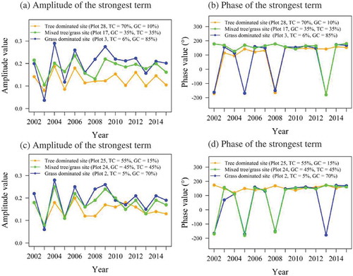
Harmonic analysis was applied to the MODIS NDVI time-series data for all 28 field plots to assess their amplitude and phase (Table 1). The strongest and second strongest harmonic terms presented here are statistically significant. There are site-specific differences in the amplitude of the strongest harmonic terms between field plots. The phase (in degrees) shows a different behaviour due to the differences in the onset of greening of the trees and grasses (Tables 1 –3). Generally, earlier green-up periods were found where tree cover was higher (e.g. plot 28 (143°) and plot 27 (145°)) and later for grass cover (e.g. plot 1 (161°) and plot 3 (164°)) in the phase of the strongest harmonic term (the annual oscillation).

Table 1. Amplitude and phase of the first and second harmonic terms of NDVI data over the field plot locations, tested with Hartley’s ANOVA F-test (α = 5%) using the Bonferroni–Holm correction (p < 0.05).

					Amplitude		Number of cycles		Phase (°)
Plot	TC (%)	GC (%)	Longitude (°)	Latitude (°)	1st	2nd	1st	2nd	1st	2nd
1	5	85	31.8632	−24.7952	0.166	0.035	14	9	161	13.3
2	5	70	31.8658	−24.7909	0.177	0.047	14	9	162	10.3
3	6	85	31.8568	−24.8024	0.182	0.042	14	5	164	−21.3
4	10.5	45	31.8540	−24.8024	0.188	0.047	14	5	162	−14.3
5	11	85	31.7916	−24.8591	0.190	0.041	14	9	158	0.75
6	11	42	31.7483	−24.9045	0.172	0.032	14	9	159	−11.3
7	12	67	31.7832	−24.8642	0.184	0.033	14	17	158	173
8	12	70	31.8411	−24.8182	0.177	0.041	14	9	161	8.95
9	17	78	31.7666	−24.8781	0.182	0.037	14	23	159	−142
10	20	70	31.7544	−24.9025	0.179	0.028	14	15	159	−43.4
11	22	35	31.7256	−24.9003	0.171	0.039	14	9	163	163
12	30	45	31.7123	−24.9122	0.199	0.037	14	15	160	−51.6
13	30	40	31.8185	−24.8366	0.181	0.044	14	9	158	−18.3
14	30	45	31.7558	−24.8990	0.177	0.029	14	15	158	−56.9
15	31	55	31.8433	−24.8155	0.174	0.042	14	9	161	4.22
16	32	35	31.8111	−24.8427	0.174	0.038	14	9	156	−16.9
17	35	35	31.6289	−24.9643	0.176	0.037	14	28	163	72.5
18	35	50	31.8206	−24.8376	0.181	0.044	14	9	157	−20.3
19	35	22	31.6948	−24.9326	0.184	0.033	14	28	161	66.6
20	35	57	31.7726	−24.8721	0.186	0.032	14	23	161	−148
21	41	35	31.8354	−24.8258	0.165	0.036	14	23	157	−15.4
22	42	30	31.7035	−24.9229	0.193	0.033	14	23	163	−160
23	45	50	31.6866	−24.9367	0.190	0.032	14	2	161	−157
24	45	45	31.8596	−24.7895	0.165	0.039	14	9	157	10.4
25	55	15	31.6374	−24.9625	0.146	0.036	14	28	152	67.6
26	65	10	31.7873	−24.7475	0.157	0.033	14	16	152	−110
27	69	20	31.8074	−24.7620	0.151	0.036	14	28	145	74.3
28	70	10	31.7487	−24.6234	0.116	0.028	14	28	143	59.7

Table 2. Significant harmonic terms of the PFTs (trees and grasses) selected with Hartley’s ANOVA F-test (p < 0.05).

Strongest terms	Tree-dominated site (plot 28)			Grass-dominated site (plot 3)
	Number of cycles	Amplitude	Phase (°)	Number of cycles	Amplitude	Phase (°)
1	14	0.115	144	14	0.182	164
2	28	0.029	−32.7	5	0.042	−21
3	10	0.028	116	9	0.040	15
4	16	0.028	64.2	23	0.036	−146
5	9	0.026	−101	16	0.035	−85.7
6	7	0.025	−112	8	0.032	−176
7	15	0.025	−14.9	17	0.031	−151
8	6	0.022	−121	39	0.030	−78.7
9	12	0.019	−52.6	7	0.029	−110
10	17	0.019	−99.6	6	0.028	−66.9

Table 3. Amplitude and phase (°) of the first harmonic term for main PFT (tree and grass) from 2002 to 2015.

	Plot 28 (TC = 70%, GC = 10%)		Plot 3 (TC = 6%, GC = 85%)		Plot 17 (TC = 35%, GC = 35%)		Plot 25 (TC = 55%, GC = 15%)		Plot 2 (TC = 5%, GC = 70%)		Plot 24 (TC = 45%, GC = 45%)
Year	Amplitude	Phase	Amplitude	Phase	Amplitude	Phase	Amplitude	Phase	Amplitude	Phase	Amplitude	Phase
2002	0.14	−171	0.20	−162	0.22	178	0.18	174	0.22	−165	0.18	−169
2003	0.08	115	0.04	156	0.10	168	0.08	148	0.06	69.5	0.08	157
2004	0.18	94.1	0.29	114	0.20	126	0.18	120	0.28	111	0.25	111
2005	0.08	142	0.11	−169	0.16	169	0.12	150	0.11	−171	0.11	−179
2006	0.18	121	0.26	159	0.24	149	0.20	139	0.25	160	0.22	153
2007	0.11	132	0.16	150	0.16	165	0.12	146	0.16	132	0.16	137
2008	0.12	−164	0.22	−150	0.13	178	0.12	169	0.24	−151	0.19	−154
2009	0.12	153	0.28	157	0.22	157	0.17	149	0.26	147	0.24	143
2010	0.15	144	0.22	154	0.20	142	0.16	138	0.19	155	0.20	153
2011	0.10	148	0.21	163	0.19	165	0.18	155	0.17	161	0.15	155
2012	0.16	144	0.22	148	0.20	164	0.16	159	0.21	150	0.19	147
2013	0.10	142	0.16	−179	0.18	−179	0.13	174	0.15	−177	0.13	173
2014	0.14	158	0.21	173	0.20	171	0.14	152	0.21	172	0.19	165
2015	0.10	153	0.20	168	0.16	180	0.13	166	0.19	169	0.17	161

Figure 5 shows 14 years of annual rainfall data for the four weather stations, their corresponding amplitude of the second strongest harmonic terms, and mean NDVI. The bar plot shows the annual rainfall for each year while the red line shows the amplitude or mean dry season MODIS NDVI. All phenology metrics respond strongly to the annual variation of rainfall.

Figure 5. Annual precipitation data from weather stations and their corresponding phenology metrics from the MODIS NDVI (2002–2015), showing Skukuza with amplitude (a) and mean dry season NDVI (b), Pafuri with amplitude (c), and mean dry season NDVI (d), Mahlengeni with amplitude (e) and mean dry season NDVI (f), SATARA with amplitude (g), and mean dry season NDVI (h).

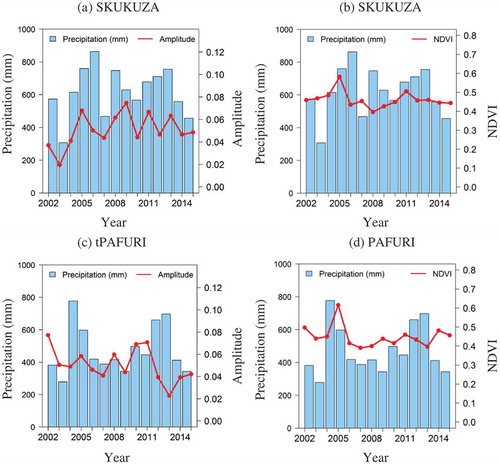
Figure 5. (Continued).

3.2.2. Comparison of strongest harmonic terms between tree- and grass-dominated plots

The amplitude indicates the productivity of the PFT, whereas the phase shows the time delay of the wave term (shift along the time axis). A comparison of the strongest significant harmonic terms between tree- and grass-dominated field plots was made regarding the 10 strongest harmonic terms. Table 2 shows distinct amplitude and phase of the PFTs for tree- and grass-dominated sites. Both exhibit a large amplitude of the strongest harmonic term but with the grass-dominated site being significantly higher than for the tree-dominated site. The cycle number corresponds to the annual seasonality over the 14 year length of the time series (cycle = 14). The PFT usually attained their most active photosynthetic stage at this time.

In the second strongest harmonic term, the tree phenology has 28 cycles, i.e. two cycles per year. Grass phenology has only five peaks over the 14 year period in the second strongest harmonic term (cycle = 5, Table 2). This implies that the amplitude of the second strongest term does not follow an annual pattern or a multiple thereof. Thus, the second strongest term shows that a subtle bimodal phenological pattern is found for tree phenology, overlaying the annual cycle, while in contrast the grass phenology has a stronger second harmonic term that does not follow an annual pattern (cycle 5). The bimodal annual signal component for grasses is found in the third strongest harmonic term (cycle 23).

3.2.3. Interannual variability of selected tree/grass productivity

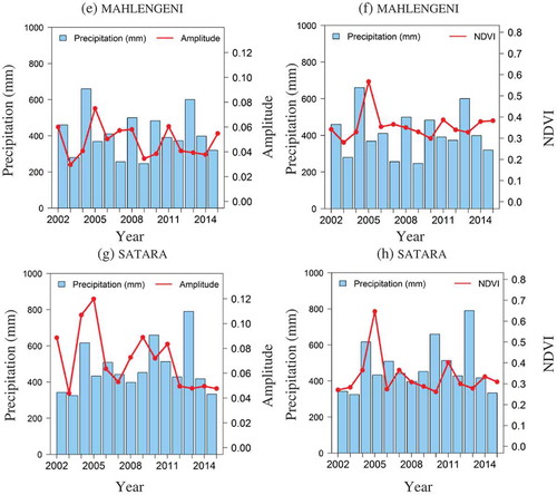
In this section, harmonic analysis was applied separately for each annual growing season (14 years separately) and each plot. The amplitude for the strongest harmonic term and its corresponding phase for six plots, tree-dominated (28, 25), grass-dominated (3, 2), and mixed tree/grass plots (17, 24) are presented in Table 3 and Figures 6(a–d). The amplitude of the strongest harmonic term for dominants PFT changes PFTs over the years. The grass-dominated plots have higher amplitude for the strongest harmonic term compared to tree-dominated plots, unless annual rainfall is low (Figure 5). The maximum amplitude value for grass-dominated plots is close to 0.29 and to 0.2 for the tree-dominated plot 25. This was2004 phenological year, which had also high precip/2004 phenological year, which had also high precipitation as (Figure 5).

Figure 6. Interannual variability of strongest harmonic terms of the decomposed tree/grass NDVI time series, computed per year. (a) Annual amplitude of the strongest term (plots 28, 18, and 10), (b) phase of the strongest term (plots 28, 18, and 10), (c) annual phase of the strongest term (plots 25, 23, and 2), and (d) phase of the strongest term (plots 25, 23, and 2).

Generally, these changes in tree/grass phenology could be seasonal (e.g. intra-annual variations due to differences in the PFT life cycle), gradual (e.g. because of climate variability), or abrupt (e.g. due to fires or drought). Regarding the phase, the greening of the PFTs changes with species and years. There are inconsistencies in the amplitude and in the greening period of the PFTs over the years. The tree-dominated plots had an earlier green-up than the grass-dominated plot (Figures 6(b)/(d)). Most tree species grow leaves (leaf flush) before the start of rainy season while most grass species depend on instantaneous water provided during the rainy season. For instance, the tree-dominated plot 28 had an earlier green-up than the grass-dominated plots for most of the years. In some years, the grass plots greened up earlier than the trees. It is unusual for grasses to have an earlier onset of greening than trees. However, this is possible when rainfall occurs earlier than usual.

3.3. Relationship between harmonic coefficients and tree/grass fractions

The main hypothesis of this study is that the harmonic coefficients contain information for discriminating the two PFTs and their respective cover. This is now examined by correlating the harmonic terms (analysis of the 14 years of MODIS NDVI data) and the tree/grass fractions estimated during the field campaign in 2015 (Table 4). All harmonic coefficient parameters showed highly significant relationships with the tree/grass fractions. Tree fractions had a strong negative correlation with amplitude (r = −0.59, p < 0.001) and phase (r = −0.73, p < 0.0001), indicating a low-growing cycle amplitude of tree-dominated plots and an earlier green-up period. The grass fractions had a strongly positive correlation with the amplitude (r = 0.51, p = 0.005) and phase (r = 0.55, p = 0.002), indicating high-growing cycle amplitude of the grass-dominated plots and later green-up period. Tree fraction was strongly correlated with the number of cycles of the second harmonic term (r = 0.56, p = 0.002), while grass fractions showed a negative correlation (r = −0.52, p = 0.005) with these cycles indicating differences in the phenological behaviour of the two PFTs due to their biological characteristics. Since the best correlation was found between tree cover and the phase of the first harmonic component, we developed a model to predict tree cover from the phase in the next sections.

Table 4. Correlation between harmonic coefficients (extracted from MODIS NDVI, 2002–2015) and tree/grass fractions estimated during the field campaign.

	Tree cover		Grass cover
Harmonic coefficients	r	p	r	p
Amplitude (1st)	−0.59	<0.001	0.51	0.005
Phase (1st)	−0.73	<0.0001	0.55	0.002
Cycles (2nd)	0.56	0.002	−0.52	0.005

3.4. Phase image

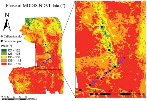
Figure 7 shows a phase image derived from the first harmonic term of the MODIS NDVI time series. The phase indicates the timing of the green-up at the start of the annual peak of the growing season. The phase in this area of KNP ranged from 121° to 150° and the green-up of the two PFTs started from the areas represented by the green colours and move towards areas with red colours in Figure 7. The spatial estimates of the phase are consistent with the distribution of tree phenological types in KNP as a function of geological formation, weather variability, and species distribution. For example, the early green-up areas are represented by the S. birrea tree savannah or A. nigrescens bush or shrub savannah Colophospermum mopane, tree savannah Karoo sediment plains (A. welwitschii tree savannah), and T. sericea bush savannah landscapes. The green-up period for the PFT in the basaltic or gabbroic plains (with shrub savannah and herbaceous plants) landscape (in the east) is late compared to the tree savannah landscapes.

Figure 7. Phase image derived from harmonic decomposition of MODIS NDVI (2002–2015).

3.5. Linear regression of phase and field data for tree cover estimate

Table 5 shows the field plots and phase used for a linear regression model of tree cover against phase. The relationship between tree cover and phase derived from the phase of 14 years of MODIS NDVI data presented a strongly linear relationship (R² = 0.51, p < 0.01, n = 14):

Table 5. Tree/grass cover data and their phase values used for the estimate.

Plot	Tree cover (%)	Grass cover (%)	Longitude (°)	Latitude (°)	Phase (°)
1	5	85	31.8632	−24.7952	145
3	6	85	31.8568	−24.8024	148
4	10.5	45	31.8540	−24.8024	146
7	12	67	31.7832	−24.8642	143
9	17	78	31.7666	−24.8781	145
10	20	70	31.7544	−24.9025	143
12	30	45	31.7123	−24.9122	144
15	31	55	31.8433	−24.8155	144
16	32	35	31.8111	−24.8427	140
19	35	22	31.6948	−24.9326	146
21	41	35	31.8354	−24.8258	143
22	42	30	31.7035	−24.9229	147
24	45	45	31.8596	−24.7895	141
27	69	20	31.8074	−24.7620	129

(2) $y=-2.769x+424.62$(2)

where y = % tree cover, and x = phase in degrees.

Although the phase variability for the field plots is not very high, plot 27 is ecologically quite different to the other plots and makes an important contribution to the model fitting. Overall, the positive relationship between the phase and per cent tree cover suggests that the model can be used to estimate per cent tree cover from the phenology data.

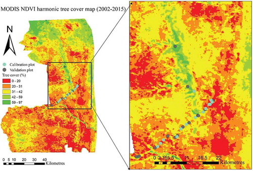
Figure 8 shows the tree cover map estimated from the phase of the strongest MODIS NDVI harmonic term and the field plot data. The map shows the heterogeneity in tree cover over KNP and the well-known boundary between the western basaltic and eastern granitic parts. Several factors such as geology, fire, herbivory, and weather variability can also have a strong impact on the density of tree cover in KNP (Smit and Asner 2012; Bucini et al. 2010).

Figure 8. Tree cover map (2002–2015) from the phase of the strongest MODIS NDVI harmonic term for the part of study area (KNP).

3.6. Validation of the tree cover map

Table 6 shows the field validation plots and their corresponding phase values, estimated tree cover, and the tree cover after Bucini (Bucini et al. 2009; Bucini et al. 2010). Figure 8 shows the accuracy assessment of the tree cover estimates. The tree estimated cover has an R² = 0.55, p < 0.01, slope = 0.93, and RMSE of 13.26% (Figure 9). The estimated tree cover showed a strong correlation with Bucini’s woody cover map (r = 78, p < 0.01, n = 14).

Table 6. Validation of the tree cover estimated from phase values and field data.

Plot	Tree cover (%)	Grass cover (%)	Longitude (°)	Latitude (°)	Phase (°)	Estimated tree cover (%)	Tree cover from Bucini (%)
2	5	70	31.8658	−24.7909	145	23.12	39.14
5	11	85	31.7916	−24.8591	142	31.42	34.79
6	11	42	31.7483	−24.9045	142	31.42	49.85
8	12	70	31.8411	−24.8182	144	25.88	35.00
11	22	35	31.7256	−24.9003	143	28.65	47.97
13	30	40	31.8185	−24.8366	142	31.42	47.40
14	30	45	31.7558	−24.8990	142	31.42	44.04
17	35	35	31.6289	−24.9643	147	17.58	48.35
18	35	50	31.8206	−24.8376	143	28.65	41.06
20	35	57	31.7726	−24.8721	145	23.12	26.18
23	45	50	31.6866	−24.9367	145	23.12	44.39
25	55	15	31.6374	−24.9625	136	48.04	60.48
26	65	10	31.7873	−24.7475	132	59.11	66.55
28	70	10	31.7487	−24.6234	128	70.19	62.97

Figure 9. Validation of the tree cover map (a) and (b) comparison of the estimated tree cover (using phase values) with Bucini’s woody cover map.

4. Discussion

This study has applied harmonic decomposition to a 14 year time series of MODIS NDVI data over a savannah transect in KNP, South Africa. The results show that the tree/grass phenology can be characterized using the amplitude, number of cycles, and phase derived from harmonic analysis (Tables 1–3, Figures 4 and 5). The greening pattern (seasonal and interannual NDVI) of the PFTs trees and grasses varies due to their differences in phenological characteristics (Tables 1–3). This was expected since PFTs respond differently to environmental conditions. For example, precipitation, fires, and herbivores influence spatial and temporal variability of vegetation inducing strong changes to annual and interannual amplitude and frequency. In these savannah ecosystems, trees usually green-up earlier in the wet season than grasses and this has been observed from the analyses of MODIS data (Tables 1 –3). Higgins et al. (2011), who identified two distinct phenological cycles for trees and grasses in KNP, explained that tree leaf flush appears to pre-empt rainfall while grass leaf flush follows the rain. The harmonic analysis here revealed that unless rainfall is particularly low grass phenology has a higher amplitude of its strongest harmonic term than tree phenology. This is caused by grasses responding more strongly to the annual seasonality of wet/dry seasons than trees, which can tap into deeper water reservoirs through their deep roots. The results also showed that phenological cycles of trees and grasses are influenced by the species types, location, and year.

The relationship between tree/grass fractions of the 28 field plots and the corresponding amplitude, phase, and number of cycles provides evidence of differences in the phenology of the two main PFT (Table 4). The relationships of trees and grasses with the harmonic coefficients manifest themselves in inverse relationships of the two PFTs with these coefficients. A previous study has demonstrated an empirical relationship between the fraction of maximum tree cover and annual grass productivity where grass density decreases as the fractional tree cover increases (Scholes 2003). A comparison of annual net primary productivity for herbaceous and shrub vegetation showed that grass-dominated sites can support higher levels of ANPP than shrubs leading to higher annual NDVI peaks (Moreno-de Las et al. 2015).

Here, we have estimated tree/grass cover in 28 plots of KNP from the amplitude, phase values, and the number of cycles of the strongest harmonic terms, excluding any terms that were not statistically significant. When applying harmonic analysis to sequences of 1 year of NDVI data, the amplitude of the two PFTs varied between years (Figures 6(a–d)). The phase values show inconsistencies in terms of the timing of the tree/grass phenology, especially in the terms that are weaker than the one with the highest amplitude (Table 3 and Figure 6(b)/(d)). The most inconsistent timing of the peak amplitude is illustrated in Figure 6(d). This might be due to an asynchronous start of the rainy season leading to grasses greening up while the trees respond more to temperatures and photoperiod (Archibald and Scholes 2007; Whitecross, Witkowski, and Archibald 2017a). Figure 5 shows that the amplitude of the strongest harmonic term is more sensitive to rainfall than the dry season NDVI. This is because the amplitudes derived from these sites reflect the more dynamic nature of the herbaceous layer, while the dry season NDVI represents more woody species. Although our study cannot conclusively attribute these changes to specific factors, it is known from the literature that the magnitude and consistency of the first and second strongest harmonic terms relate to secondary succession, weather anomalies, and other land-cover changes (Moody and Johnson 2001). Similarly, Jakubauskas, Legates, and Kastens (2001) explained that changes in harmonic parameters (especially amplitude and phase) can indicate changes in the natural vegetation, e.g. in terms of maximum greenness (due to onset of greenness), or changes in vegetation condition due to drought, flooding, or overgrazing or land surface condition (changes arising from post-fire regeneration, natural or anthropogenic disturbance). Furthermore, climate, soil nutrients, and fire are some of the most essential components influencing savannah vegetation dynamics (February et al. 2005). A recent study by Whitecraoss et al. (2017a), which assessed the frequency and drivers of early greening in broad-leaved woodlands, explained that the rainfall variability, compared to photoperiod and temperature, had the strongest influence over a latitudinal gradient in southern Africa.

The moderate relationship between the phase of the averaged 14 year MODIS NDVI and the tree-dominated field plots indicates the usefulness of harmonic analysis for estimating tree cover in savannahs (Table 4). The tree cover estimated in this study also shows a strong correlation with a previous woody cover map by Bucini (Bucini et al. 2009; Bucini et al. 2010) (Figure 9). Although NDVI values have been reported as being suboptimal for FVC estimation (Jiang et al. 2006), some methods that account for soil background contribution in the NDVI have shown good relationships with ground measurements (Moreno-de Las et al. 2015; Ding et al. 2016; Zeng et al. 2000). However, signal contamination, soil background colour, and saturation problems limited the NDVI–FVC relationship (Verger et al. 2009; Baumgardner et al. 1986). The use of phase to estimate tree cover through empirical methods is an important contribution to remote sensing of tree/grass fractional cover estimations as the effects of soil backgrounds remain a significant challenge in the estimate cover fractions especially when using vegetation indices (Ding et al. 2016; Cho, Ramoelo, and Dziba 2017). It is also important because of the increased demand for reliable tree fractional cover products to be used in model parameterization and validation (Boke-Olén et al. 2016).

Harmonic analysis has been described as being limited due to its demand for prior ecological knowledge, long-term data sets, and the need for effective interpretation of confidence intervals of the observations in the power spectrum (de Beurs and Henebry 2010). Again, despite careful experimental planning, a pixel-level analysis in remote sensing and GIS is subject to some remaining uncertainties depending on the data sets and modelling approaches (Fisher 1997). Our study recognizes these limitations and adopts approaches to minimize them. A long-term data set of over a decade was interpreted using field information collected in 1 year. Uncertainty in this kind of phenology analysis has three main components:

1. uncertainty in geolocation of the field plot locations and satellite pixels when matching NDVI time series to fractional cover data from plots;

2. uncertainty in how the tree/grass cover inside the field plots may have changed over the 14 years; and

3. uncertainty inherent in the NDVI measurements from the MODIS sensor, e.g. variability resulting from sensor viewing geometry or attenuation of the signal by tree canopies (McCoy 2005; Gill et al. 2009; Los et al. 2005).

First, since the field survey has considered the MODIS satellite pixel size by sampling plot of almost equal to the size of the pixel, the centres of the plots were chosen such that they are representative of a large surrounding area and that the point data were georeferenced to the projection system of MODIS; the first uncertainty term is considered minimal. Second, the use of recent field data for mapping annual and interannual tree/grass phenology in savannah may lead to increase uncertainty although tree phenology is more stable over time than grass cover. While our results demonstrated the potential of MODIS data to estimate per cent tree cover from vegetation indices using signal decomposition (Figure 9: R² = 0.55, p < 0.01, slope = 0.93, with RMSE = 13.26%), the estimates of tree cover from the phase values have RMSE = 13.26%, which is partly due to the presence of certain late-flushing tree species that green-up later than trees usually do, making their phenology similar to grasses (Higgins et al. 2011). In addition, the estimated tree cover in this study is an average of 14 year MODIS NDVI data. Specifically, tree phenology is influenced mainly by temperature and day length (Chidumayo, 2001; Whitecross, Witkowski, and Archibald 2017a), or precipitation and disturbance in certain condition (February et al. 2005; Whitecross, Witkowski, and Archibald 2017b). Therefore, changes in tree/grass phenology due to high interannual variability (seasonality, fires, and drought) in savannah may have important implication for tree cover estimates. In savannah, high variability of the herbaceous layer is reflected in the overall phenological signal of a plot and this can affect the tree/grass separation method (Whitecross, Witkowski, and Archibald 2017a; Whitecross, Witkowski, and Archibald 2017b). Even though there can be small changes in the amplitude mostly contributed by the grass layer (Scanlon et al. 2002), the use of a composite data set (Holben 1986; Hilker et al. 2009) is more promising than a single-date data set (Mondal et al. 2014) Although the lidar/SAR tree product, tree cover estimated using harmonic analysis (with estimated tree cover by Bucini), and the lidar/SAR data had strong correlation with field data, the level of uncertainty in the estimates from these products compared to field data is probably due to time gap between the remote-sensing data and the time of the field campaign. For example, the Bucini woody cover map was produced from the Landsat data acquired between 2000 and 2001 and the JERS-1 SAR scenes (L-band, HH polarization) were acquired between 1995 and 1996. The MODIS NDVI was acquired from 2002 to 2015 while the field campaign for this study was in 2015. The time gap means that there could be differences in the density of tree cover in KNP over this period. Third, for MODIS data product MOD13Q1, the influence of viewing geometry on vegetation indices has been investigated and was found to be less significant with NDVI than individual channel (Los et al. 2005; Gill et al. 2009).

The amplitude, phase values, and the cycles of the strongest harmonic terms characterize tree/grass phenology for the KNP study sites. This study shows that harmonic analysis can discriminate between tree- and grass-dominated savannahs. Tests in other savannah types will show whether it is sufficiently robust to retrieve FVC of trees and grasses at continental scale. The quantitative analysis of tree/grass phenology from satellite time-series data enables a better understanding of the dynamics of the tree/grass competition and coexistence.

5. Conclusions

Harmonic analysis was applied to estimate fractional cover of tree/grass PFTs in KNP. MODIS NDVI time-series data over 14 years have shown that the statistically significant harmonic terms, with amplitude, cycles, and phase values, show distinct patterns for trees and for grasses. The harmonic coefficients of the strongest harmonic term were robust discriminators between tree and grass phenology because grasses respond more strongly to the annual seasonal cycle than trees. The phase values show that trees green up earlier than grasses. The research also demonstrated how the phase values for tree phenology from satellite remote sensing can be used to estimate fractional cover (R² = 0.55, p < 0.01, slope = 0.93, RMSE = 13.26%).

Limitations inherent in this analysis include the relatively small number of field plots. More effort should therefore go into defining the empirical relationship between tree/grass fractional cover and satellite phenology metrics perhaps comparing different approaches.

Acknowledgments

This study was partially funded by the Natural Environment Research Council’s support for the National Centre for Earth Observation. H. Balzter was supported by the Royal Society Wolfson Research Merit Award, 2011/R3 and the NERC National Centre for Earth Observation. We wish to thank the South African National Parks for granting field work permission in the Kruger National Park (KNP). We also wish to thank Izak Smit and Chenay Simms for providing GIS data for KNP. Special thanks to National Aeronautics and Space Administration (NASA) for providing the MODIS data.

Disclosure statement

No potential conflict of interest was reported by the authors.

Additional information

Funding

This study was partially funded by the Natural Environment Research Council’s support for the National Centre for Earth Observation. H. Balzter was supported by the Royal Society Wolfson Research Merit Award, 2011/R3 and the NERC National Centre for Earth Observation.

References

- Accatino, F., C. De Michele, R. Vezzoli, D. Donzelli, and R. J. Scholes. 2010. “Tree-Grass Co-Existence in Savanna: Interactions of Rain and Fire.” Journal of Theoretical Biology 267 (2): 235–242. doi:10.1016/j.jtbi.2010.08.012.
- Andres, L., W. A. Salas, and D. Skole. 1994. “Fourier Analysis of Multi-Temporal AVHRR Data Applied to a Land Cover Classification.” Remote Sensing 15 (5): 1115–1121. doi:10.1080/01431169408954145.
- Archibald, S., and R. J. Scholes. 2007. “Leaf Green-Up in a Semi-Arid African Savanna Separating Tree and Grass Responses to Environmental Cues.” Journal of Vegetation Science 18 (4): 583–594. doi:10.1658/1100-9233(2007)18[583:LGIASA]2.0.CO;2.
- Asner, G. P., S. R. Levick, T. Kennedy-Bowdoin, D. E. Knapp, R. Emerson, J. Jacobson, M. S. Colgan, and R. E. Martin. 2009. “Large-Scale Impacts of Herbivores on the Structural Diversity of African Savannas.” Proceedings of the National Academy of Sciences 106 (12): 4947–4952. doi:10.1073/pnas.0810637106.
- Balzter, H., F. Gerard, C. George, G. Weedon, W. Grey, B. Combal, E. Bartholomé, S. Bartalev, and S. Los. 2007. “Coupling of Vegetation Growing Season Anomalies and Fire Activity with Hemispheric and Regional-Scale Climate Patterns in Central and East Siberia.” Journal of Climate 20 (15): 3713–3729. doi:10.1175/JCLI4226.
- Baumgardner, M. F., L. F. Silva, L. L. Biehl, and E. R. Stoner. 1986. “Reflectance Properties of Soils.” In Advances in Agronomy, edited by N. C. Brady, 1–44. San Diego, USA: Academic Press.
- Bloomfield, P. 2004. Fourier Analysis of Time Series: An Introduction. New York, NY: John Wiley & Sons.
- Boke-Olén, N., V. Lehsten, J. Ardö, J. Beringer, L. Eklundh, T. Holst, E. Veenendaal, and T. Tagesson. 2016. “Estimating and Analyzing Savannah Phenology with a Lagged Time Series Model.” PloS One 11 (4): e0154615. doi:10.1371/journal.pone.0154615.
- Bond, W. J., and J. E. Keeley. 2005. “Fire as a Global ‘Herbivore’: The Ecology and Evolution of Flammable Ecosystems.” Trends in Ecology & Evolution 20 (7): 387–394. doi:10.1016/j.tree.2005.04.025.
- Bucini, G., N. P. Hanan, R. B. Boone, I. P. J. Smit, S. Saatchi, M. A. Lefsky, and G. P. Asner. 2010. “Woody Fractional Cover in Kruger National Park, South Africa: Remote-Sensing-Based Maps and Ecological Insights.” In Ecosystem Function in Savannas: Measurement and Modeling at Landscape to Global Scales, edited by Hill, M. J. and N. P. Hanan. 219–238.
- Bucini, G., S. Saatchi, N. Hanan, R. B. Boone, and I. Smit. 2009. “Woody Cover and Heterogeneity in the Savannas of the Kruger National Park, South Africa.” Proceedings from the 2009 IEEE International Geoscience and Remote Sensing Symposium IV, Cape Town, South Africa, July 12–17, pp. 334–337.
- Canisius, F., H. Turral, and D. Molden. 2007. “Fourier Analysis of Historical NOAA Time Series Data to Estimate Bimodal Agriculture.” International Journal of Remote Sensing 28 (24): 5503–5522. doi:10.1080/01431160601086043.
- Chamaille-Jammes, S., and H. Fritz. 2009. “Precipitation-NDVI Relationships in Eastern and Southern African Savannas Vary along a Precipitation Gradient.” International Journal of Remote Sensing 30 (13): 3409–3422. doi:10.1080/01431160802562206.
- Chamaille-Jammes, S., H. Fritz, and F. Murindagomo. 2006. “Spatial Patterns of the NDVI-rainfall Relationship at the Seasonal and Interannual Time Scales in an African Savanna.” International Journal of Remote Sensing 27 (23): 5185–5200. doi:10.1080/01431160600702392.
- Chidumayo, E.N. 2001. “Climate And Phenology of Savanna Vegetation in Southern Africa.” Journal of Vegetation Science 12 (3): 347-354. doi:10.2307/3236848.
- Cho, M. A., A. Ramoelo, and L. Dziba. 2017. “Response of Land Surface Phenology to Variation in Tree Cover during Green-Up and Senescence Periods in the Semi-Arid Savanna of Southern Africa.” Remote Sens 9 (7): 689. doi:10.3390/rs9070689.
- Cho, M. A., R. Mathieu, G. P. Asner, L. Naidoo, J. Van Aardt, A. Ramoelo, P. Debba, K. Wessels, R. Main, I. P. Smit, and B. Erasmus. 2012. “Mapping Tree Species Composition in South African Savannas Using an Integrated Airborne Spectral and LiDAR System.” Remote Sensing of Environment 125 :214–226. doi:10.1016/j.rse.2012.07.010.
- Cleland, E. E., I. Chuine, A. Menzel, H. A. Mooney, and M. D. Schwartz. 2007. “Shifting Plant Phenology in Response to Global Change.” Trends in Ecology & Evolution 22 (7): 357–365. doi:10.1016/j.tree.2007.04.003.
- Cleveland, R. B., W. S. Cleveland, J. E. McRae, and I. Terpenning. 1990. “STL: A Seasonal-Trend Decomposition Procedure Based on Loess.” Journal of Official Statistics 6 (1): 3–73.
- de Beurs, K. M., and G. M. Henebry. 2010. “Spatio-Temporal Statistical Methods for Modelling Land Surface Phenology.” In Phenological Research, edited by Hudson, I.L. and M. R. Keatley. 177–208. Dordrecht: Springer.
- Ding, Y., X. Zheng, K. Zhao, X. Xin, and H. Liu. 2016. “Quantifying the Impact of NDVIsoil Determination Methods and NDVIsoil Variability on the Estimation of Fractional Vegetation Cover in Northeast China.” Remote Sensing 8 (1): 29. doi:10.3390/rs8010029.
- Eckhardt, H. C., B. W. Van Wilgen, and H. Biggs. 2000. “Trends in Woody Vegetation Cover in the Kruger National Park, South Africa, between 1940 and 1998.” African Journal of Ecology 38: 108–115. Review of. doi:10.1046/j.1365-2028.2000.00217.x.
- Eklundha, L., and J. Per. 2012. TIMESAT 3.1 Software Manual. Sweden : Lund University.
- February, E. C., P. G. H. Frost, M. Sankaran, A. Diouf, C. J. Feral, B. S. Cade, H. H. T. Prins, et al. 2005. “Determinants of Woody Cover in African Savannas.” Nature 438 (7069): 846–849. doi:10.1038/nature04070.
- Fisher, P. 1997. “The Pixel: A Snare and A Delusion.” International Journal of Remote Sensing 18 (3): 679–685. doi:10.1080/014311697219015.
- Foody, G. M. 2003. “Geographical Weighting as a Further Refinement to Regression Modelling: An Example Focused on the NDVI–Rainfall Relationship.” Remote Sensing of Environment 88 (3): 283–293. doi:10.1016/j.rse.2003.08.004.
- Gessner U., C. Conrad, C. Hüttich, M. Keil, M. Schmidt, M. Schramm, and S. Dech. 2008. A Multi-Scale Approch for Retreiving Proportional Cover of Life Forms. Paper presented at the Geoscience and Remote Sensing Symposium, IGARSS 2008, July 6-11, Boston, USA. pp. 4. IEEE International.
- Gill, T. K., S. R. Phinn, J. D. Armston, and B. A. Pailthorpe. 2009. “Estimating Tree-Cover Change in Australia: Challenges of Using the MODIS Vegetation Index Product.” International Journal of Remote Sensing 30 (6): 1547–1565. doi:10.1080/01431160802509066.
- Hartley, H. O. 1949. “Tests of Significance in Harmonic Analysis.” Biometrika 36: 194–201. doi:10.1093/biomet/36.1-2.194.
- Hernandez-Leal, P. A., M. Arbelo, and A. Gonzalez-Calvo. 2006. “Fire Risk Assessment Using Satellite Data.” Advances in Space Research 37 (4): 741–746. doi:10.1016/j.asr.2004.12.053.
- Higgins, S. I., M. D. Delgado-Cartay, E. C. February, and H. J. Combrink. 2011. “Is There a Temporal Niche Separation in the Leaf Phenology of Savanna Trees and Grasses?” Journal of Biogeography 38 (11): 2165–2175. doi:10.1111/j.1365-2699.2011.02549.x.
- Hilker, T., M. A. Wulder, N. C. Coops, J. Linke, G. McDermid, J. G. Masek, F. Gao, and J. C. White. 2009. “A New Data Fusion Model for High Spatial-And Temporal-Resolution Mapping of Forest Disturbance Based on Landsat and MODIS.” Remote Sensing of Environment 113 (8): 1613–1627. doi:10.1016/j.rse.2009.03.007.
- Hill, M. J., M. O. Román, C. B. Schaaf, L. Hutley, C. Brannstrom, A. Etter, and N. P. Hanan. 2011. “Characterizing Vegetation Cover in Global Savannas with an Annual Foliage Clumping Index Derived from the MODIS BRDF Product.” Remote Sensing of Environment 115 (8): 2008–2024. doi:10.1016/j.rse.2011.04.003.
- Hill, M. J., and N. P. Hanan. 2010. Ecosystem Function in Savannas: Measurement and Modeling at Landscape to Global Scales: New York, NY: CRC Press.
- Holben, B. N. 1986. “Characteristics of Maximum-Value Composite Images from Temporal AVHRR Data.” International Journal of Remote Sensing 7 (11): 1417–1434. doi:10.1080/01431168608948945.
- Jakubauskas, M., and R. L. E. G. A. T. E. S. David. 2000. “Harmonic Analysis of Time-Series AVHRR NDVI Data for Characterizing US Great Plains Land Use/Land Cover.” International Archives of Photogrammetry and Remote Sensing 33 (B4/1; PART 4): 384–389.
- Jakubauskas, M. E., D. R. Legates, and J. H. Kastens. 2001. “Harmonic Analysis of Time-Series AVHRR NDVI Data.” Photogrammetric Engineering and Remote Sensing 67 (4): 461–470.
- Jakubauskas, M. E., D. R. Legates, and J. H. Kastens. 2002. “Crop Identification Using Harmonic Analysis of Time-Series AVHRR NDVI Data.” Computers and Electronics in Agriculture 37 (1): 127–139. doi:10.1016/S0168-1699(02)00116-3.
- Jiang, Z., A. R. Huete, J. Chen, Y. Chen, J. Li, G. Yan, and X. Zhang. 2006. “Analysis of NDVI and Scaled Difference Vegetation Index Retrievals of Vegetation Fraction.” Remote Sensing of Environment 101 (3): 366–378. doi:10.1016/j.rse.2006.01.003.
- Jung, M., and E. Chang. 2015. “NDVI-based Land-Cover Change Detection Using Harmonic Analysis.” International Journal of Remote Sensing 36 (4): 1097–1113.
- Khalefa, E., P. J. Izak, A. N. Smit, S. Archibald, A. Comber, and H. Balzter. 2013. “Retrieval of Savanna Vegetation Canopy Height from ICESat-GLAS Spaceborne LiDAR with Terrain Correction.” IEEE Geoscience and Remote Sensing Letters 10: 1439–1443. doi:10.1109/LGRS.2013.2259793.
- Köhl, M., S. S. Magnussen, and M. Marchetti. 2006. Sampling Methods, Remote Sensing and GIS Multiresource Forest Inventory. London: Springer Science & Business Media.
- Kostadinov, T. S., A. Cabré, H. Vedantham, I. Marinov, A. Bracher, R. J. W. Brewin, A. Bricaud, et al. 2017. “Inter-Comparison of Phytoplankton Functional Type Phenology Metrics Derived from Ocean Color Algorithms and Earth System Models.” Remote Sensing of Environment 190: 162–177. doi:10.1016/j.rse.2016.11.014.
- Law, B. E., T. Arkebauer, J. L. Campbell, J. Chen, O. Sun, M. Schwartz, C. Van Ingen, and S. Verma. 2008. “Terrestrial Carbon Observations: Protocols for Vegetation Sampling and Data Submission.” FAO, Rome.
- Los, S. O., P. R. J. North, W. M. F. Grey, and M. J. Barnsley. 2005. “A Method to Convert AVHRR Normalized Difference Vegetation Index Time Series to A Standard Viewing and Illumination Geometry.” Remote Sensing of Environment 99 (4): 400–411. doi:10.1016/j.rse.2005.08.017.
- Lu, H., M. R. Raupach, T. R. McVicar, and D. J. Barrett. 2003. “Decomposition of Vegetation Cover into Woody and Herbaceous Components Using AVHRR NDVI Time Series.” Remote Sensing of Environment 86 (1): 1–18. doi:10.1016/S0034-4257(03)00054-3.
- Mairota, P., B. Cafarelli, R. K. Didham, F. P. Lovergine, R. M. Lucas, H. Nagendra, D. Rocchini, and C. Tarantino. 2015. “Challenges and Opportunities in Harnessing Satellite Remote-Sensing for Biodiversity Monitoring.” Ecological Informatics 30: 207–214. doi:10.1016/j.ecoinf.2015.08.006.
- Martínez, B., and M. A. Gilabert. 2009. “Vegetation Dynamics from NDVI Time Series Analysis Using the Wavelet Transform.” Remote Sensing of Environment 113 (9): 1823–1842. doi:10.1016/j.rse.2009.04.016.
- Mathieu, R., L. Naidoo, M. A. Cho, B. Leblon, R. Main, K. Wessels, G. P. Asner, J. Buckley, J. Van AardT, and B. F. Erasmus. 2013. “Toward Structural Assessment of Semi-Arid African Savannahs and Woodlands: The Potential of Multitemporal Polarimetric RADARSAT-2 Fine Beam Images.” Remote Sensing of Environment 138: 215–231. doi:10.1016/j.rse.2013.07.011.
- McCoy, R. M. 2005. Field Methods in Remote Sensing. New York, NY: Guilford Press.
- Mingwei, Z., Z. Qingbo, C. Zhongxin, L. Jia, Z. Yong, and C. Chongfa. 2008. “Crop Discrimination in Northern China with Double Cropping Systems Using Fourier Analysis of Time-Series MODIS Data.” International Journal of Applied Earth Observation and Geoinformation 10 (4): 476–485. doi:10.1016/j.jag.2007.11.002.
- Mondal, S., C. Jeganathan, N. K. Sinha, H. Rajan, T. Roy, and P. Kumar. 2014. “Extracting Seasonal Cropping Patterns Using Multi-Temporal Vegetation Indices from IRS LISS-III Data in Muzaffarpur District of Bihar, India.” The Egyptian Journal of Remote Sensing and Space Science 17 (2): 123–134. doi:10.1016/j.ejrs.2014.09.002.
- Moody, A., and D. M. Johnson. 2001. “Land-Surface Phenologies from AVHRR Using the Discrete Fourier Transform.” Remote Sensing of Environment 75 (3): 305–323. doi:10.1016/S0034-4257(00)00175-9.
- Moreno-de Las, H., M. R. Díaz-Sierra, L. Turnbull, and J. Wainwright. 2015. “Assessing Vegetation Structure and ANPP Dynamics in a Grassland-Shrubland Chihuahuan Ecotone Using NDVI-rainfall Relationships.” Biogeosciences Discussions 12 (1): 51–92. doi:10.5194/bgd-12-51-2015.
- Muñoz Peña, M. A., and F. A. R. Navarro. 2016. “An NDVI-data Harmonic Analysis to Study Deforestation in Peru’s Tahuamanu Province during 2001–2011.” International Journal of Remote Sensing 37 (4): 856–875. doi:10.1080/01431161.2015.1136446.
- Naidoo, L., R. Mathieu, R. Main, W. Kleynhans, K. Wessels, G. Asner, and B. Leblon. 2015. “Savannah Woody Structure Modelling and Mapping Using Multi-Frequency (X-, C-And L-Band) Synthetic Aperture Radar Data.” ISPRS Journal of Photogrammetry and Remote Sensing 105: 234–250. doi:10.1016/j.isprsjprs.2015.04.007.
- Reed, B. C., J. F. Brown, D. VanderZee, T. R. Loveland, J. W. Merchant, and D. O. Ohlen. 1994. “Measuring Phenological Variability from Satellite Imagery.” Journal of Vegetation Science 5 (5): 703–714. doi:10.2307/3235884.
- Riemann, R., G. Liknes, J. O’neil-Dunne, C. Toney, and T. Lister. 2016. “Comparative Assessment of Methods for Estimating Tree Canopy Cover across a Rural-To-Urban Gradient in the mid-Atlantic Region of the USA.” Environmental Monitoring and Assessment 188: 1–17. doi:10.1007/s10661-016-5281-8.
- Roderick, M. L., I. R. Noble, and S. W. Cridland. 1999. “Estimating Woody and Herbaceous Vegetation Cover from Time Series Satellite Observations.” Global Ecology and Biogeography 8 (6): 501–508. doi:10.1046/j.1365-2699.1999.00153.x.
- Sankaran, M., J. Ratnam, and N. Hanan. 2008. “Woody Cover in African Savannas: The Role of Resources, Fire and Herbivory.” Global Ecology and Biogeography 17 (2): 236–245. doi:10.1111/geb.2008.17.issue-2.
- Scanlon, T. M., J. D. Albertson, K. K. Caylor, and C. A. Williams. 2002. “Determining Land Surface Fractional Cover from NDVI and Rainfall Time Series for a Savanna Ecosystem.” Remote Sensing of Environment 82 (2): 376–388. doi:10.1016/S0034-4257(02)00054-8.
- Scharlemann, J. P. W., D. Benz, S. I. Hay, B. V. Purse, A. J. Tatem, G. R. William Wint, and D. J. Rogers. 2008. “Global Data for Ecology and Epidemiology: A Novel Algorithm for Temporal Fourier Processing MODIS Data.” PloS One 3 (1): 1408. doi:10.1371/journal.pone.0001408.
- Scholes, R. J. 2003. “Convex Relationships in Ecosystems Containing Mixtures of Trees and Grass.” Environmental and Resource Economics 26 (4): 559–574. doi:10.1023/B:EARE.0000007349.67564.b3.
- Scholes, R. J., and S. R. Archer. 1997. “Tree-Grass Interactions in Savannas.” Annual Review of Ecology and Systematics 28: 517–544. doi:10.1146/annurev.ecolsys.28.1.517.
- Smit, I. P. J., and G. P. Asner. 2012. “Roads Increase Woody Cover under Varying Geological, Rainfall and Fire Regimes in African Savanna.” Journal of Arid Environments 80: 74–80. doi:10.1016/j.jaridenv.2011.11.026.
- Smit, I. P. J., G. P. Asner, N. Govender, T. Kennedy-Bowdoin, D. E. Knapp, and J. Jacobson. 2010. “Effects of Fire on Woody Vegetation Structure in African Savanna.” Ecological Applications 20 (7): 1865–1875. doi:10.1890/09-0929.1.
- Smith, A. M. S., C. A. Kolden, W. T. Tinkham, A. F. Talhelm, J. D. Marshall, A. T. Hudak, L. Boschetti, et al. 2014b. “Remote Sensing the Vulnerability of Vegetation in Natural Terrestrial Ecosystems.” Remote Sensing of Environment 154 :322–337. doi:10.1016/j.rse.2014.03.038.
- Smith, A. M. S., M. J. Falkowski, J. A. Greenberg, and W. T. Tinkham. 2014a. “Remote Sensing of Vegetation Structure, Function, and Condition: Special Issue.” Remote Sensing of Environment 154: 319–321. doi:10.1016/j.rse.2014.05.002.
- Tucker, C. J., and P. J. Sellers. 1986. “Satellite Remote Sensing of Primary Production.” International Journal of Remote Sensing 7 (11): 1395–1416. doi:10.1080/01431168608948944.
- Verbesselt, J., R. Hyndman, G. Newnham, and D. Culvenor. 2010. “Detecting Trend and Seasonal Changes in Satellite Image Time Series.” Remote Sensing of Environment 114 (1): 106–115. doi:10.1016/j.rse.2009.08.014.
- Verger, A., B. Martínez, F. Camacho‐De Coca, and F. J. García‐Haro. 2009. “Accuracy Assessment of Fraction of Vegetation Cover and Leaf Area Index Estimates from Pragmatic Methods in a Cropland Area.” International Journal of Remote Sensing 30 (10): 2685–2704. doi:10.1080/01431160802555804.
- Westra, T., and R. R. De Wulf. 2007. “Monitoring Sahelian Floodplains Using Fourier Analysis of MODIS Time‐Series Data and Artificial Neural Networks.” International Journal of Remote Sensing 28 (7): 1595–1610. doi:10.1080/01431160600887698.
- White, M. A., and R. R. Nemani. 2006. “Real-Time Monitoring and Short-Term Forecasting of Land Surface Phenology.” Remote Sensing of Environment 104 (1): 43–49. doi:10.1016/j.rse.2006.04.014.
- Whitecross, M. A., E. T. F. Witkowski, and S. Archibald. 2017a. “Assessing the Frequency and Drivers of Early-Greening in Broad-Leaved Woodlands along a Latitudinal Gradient in Southern Africa.”.” Austral Ecology 42:: 341–353. doi:10.1111/aec.12448.
- Whitecross, M. A., E. T. F. Witkowski, and S. Archibald. 2017b. “Savanna Tree-Grass Interactions: A Phenological Investigation of Green-Up in Relation to Water Availability over Three Seasons.” South African Journal of Botany 108: 29–40. doi:10.1016/j.sajb.2016.09.003.
- Yang, J., P. J. Weisberg, and N. A. Bristow. 2012. “Landsat Remote Sensing Approaches for Monitoring Long-Term Tree Cover Dynamics in Semi-Arid Woodlands: Comparison of Vegetation Indices and Spectral Mixture Analysis.” Remote Sensing of Environment 119: 62–71. doi:10.1016/j.rse.2011.12.004.
- Zeng, X., R. E. Dickinson, A. Walker, M. Shaikh, R. S. DeFries, and Q. Jiaguo. 2000. “Derivation and Evaluation of Global 1-Km Fractional Vegetation Cover Data for Land Modeling.” Journal of Applied Meteorology 39 (6): 826–839. doi:10.1175/1520-0450(2000)039<0826:DAEOGK>2.0.CO;2.