Implementation of machine-learning classification in remote sensing: an applied review

ABSTRACT

Machine learning offers the potential for effective and efficient classification of remotely sensed imagery. The strengths of machine learning include the capacity to handle data of high dimensionality and to map classes with very complex characteristics. Nevertheless, implementing a machine-learning classification is not straightforward, and the literature provides conflicting advice regarding many key issues. This article therefore provides an overview of machine learning from an applied perspective. We focus on the relatively mature methods of support vector machines, single decision trees (DTs), Random Forests, boosted DTs, artificial neural networks, and k-nearest neighbours (k-NN). Issues considered include the choice of algorithm, training data requirements, user-defined parameter selection and optimization, feature space impacts and reduction, and computational costs. We illustrate these issues through applying machine-learning classification to two publically available remotely sensed data sets.

KEYWORDS:

• Land-cover classification
• image classification
• land-cover mapping
• machine learning

1. Introduction

Machine-learning classification has become a major focus of the remote-sensing literature (e.g. Pal and Mather 2003; 2005; Pal 2005; Mountrakis, Im, and Ogole 2011; Belgiu and Drăguţ 2016). Machine-learning algorithms are generally able to model complex class signatures, can accept a variety of input predictor data, and do not make assumptions about the data distribution (i.e. are nonparametric). A wide range of studies have generally found that these methods tend to produce higher accuracy compared to traditional parametric classifiers, especially for complex data with a high-dimensional feature space, i.e. many predictor variables (e.g. Hansen, Dubayah, and DeFries 1996; Friedl and Brodley 1997; Hansen and Reed 2000; Huang, Davis, and Townshend 2002; Rogan et al. 2003; Pal 2005; Pal and Mather 2005; Ghimire et al. 2012). Machine-learning approaches have become widely accepted, as is evidenced by their use in operational land-cover mapping. For example, the 2001 National Land-Cover Database (NLCD) land-cover classification for the contiguous USA was produced using decision trees (DTs) (Homer et al. 2004).

Despite the increasing acceptance of machine-learning classifiers, parametric methods appear still to be commonly used in application articles and remain one of the major standards for benchmarking classification experiments. For example, in a meta-analysis of 1651 articles that compared remote-sensing classifications methods, Yu et al. (2014) found that the parametric maximum likelihood (ML) classifier was the most commonly used method, employed in 32% of the articles, even though machine-learning methods were routinely found to have notably higher accuracies than ML. Yu et al. (2014) attribute this dominance of ML to its wide availability in conventional remote-sensing image-processing software packages and call for further software development and training relating to machine learning. Our anecdotal experience in working with users of remotely sensed data supports this argument. Indeed, we have found that uncertainties regarding how to use and implement machine-learning techniques effectively are the principal barrier for their use by many application scientists.

These uncertainties exist despite the large number of remote-sensing research articles that have investigated machine learning for classification in remote sensing. This includes a number of excellent review articles for specific methods, such as Mountrakis, Im, and Ogole (2011) review of support vector machines (SVMs), and Belgiu and Drăguţ (2016) article about Random Forests (RFs), as well as articles reviewing the process of classification and its complexities, such as that of Lu and Weng (2007). Ghamisi et al. (2017) offer a recent review of advanced algorithms with a focus on the classification of hyperspectral data that compare and highlight the strengths and weaknesses of a variety of methods. Nevertheless, a broad discussion with an applied perspective, focused on how to use these algorithms, is not to our knowledge currently available in the academic literature. Therefore, this article reviews the machine-learning literature and explores practical considerations regarding the use of machine learning for remote-sensing classification.

Our review by design focuses on six relatively mature machine-learning methods: SVMs, single DTs, RFs, boosted DTs, artificial neural networks (ANNs), and k-nearest neighbour (k-NN). We do not consider the many new machine-learning algorithms [e.g. extreme learning machines (kernel-based extreme learning machines (KELMs)) (Pal, Maxwell, and Warner 2013) and deep convolution neural networks (Yue et al. 2015)], because such methods have not yet been widely adopted. Instead, our review focuses on methods that are relatively well understood and that have been extensively tested, including in operational (i.e. non-research) settings.

2. Example machine-learning classifications

In order to explore the complexities and nuances of the issues raised in the literature, we employ two publically available data sets that we classify with each of the six different algorithms that are the focus of this article. The classifications were carried out using the free statistical software tool R (R Core Development Team 2016). Within R, we used the caret package (Kuhn et al. 2016), which provides a standard syntax to execute a variety of machine-learning methods, thus simplifying the process of systematically comparing different algorithms and approaches. Table 1 lists the R packages that caret uses to execute each of the algorithms discussed in this article. Example code from our implementation is provided in the supplemental material, as Appendices 1–4. R is not the only tool that could be used in this endeavour; other software tools, such as scikit-learn for Python and Weka, could also potentially be used (see Section 9, for additional details).

Table 1. R packages used by caret.

Algorithm	Package	Citation
RF	Ranger	Wright (2017)
SVM	Kernlab	Karatzoglou, Smola, and Hornik (2016)
DT	Rpart	Therneau, Atkinson, and Ripley (2017)
Boosted DT	C50	Kuhn et al. (2015)
ANN	Nnet	Ripley and Venables (2016)
k-NN	Caret	Kuhn et al. (2016)

2.1. Indian Pines data set

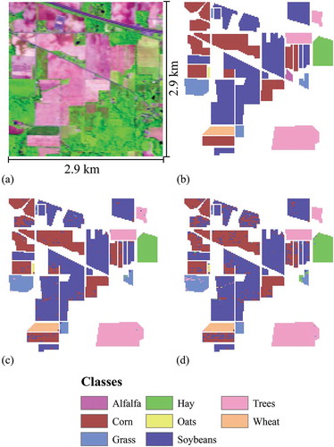
The Indian Pines Airborne Visible/Infrared Imaging Spectrometer (AVIRIS) imagery and associated ground reference data are made available by Purdue University (https://engineering.purdue.edu/~biehl/MultiSpec/hyperspectral.html). This hyperspectral data set has 220 spectral bands and 20 m pixels. The imagery was collected on 12 June 1992 and represents a 2.9 by 2.9 km area in Tippecanoe County, Indiana, USA. This is primarily an agricultural area, and eight classes are differentiated: alfalfa, corn, grass, hay, oats, soybeans, trees, and wheat (Baumgardner, Biehl, and Landgrebe 2015) (Figure 1). The Indian Pines data set has been used in numerous prior publications and has become a de facto standard for testing and comparing algorithms. We chose this data set not only because it is well known but also because the area, and thus the number of reference samples, varies greatly among the classes (Table 2), a condition known as an imbalanced training set. In our use of the Indian Pines data, pixels were separated into training and test samples using random sampling stratified by class, with 2287 pixels (25%) used to train the model, and 6857 pixels (75%) used to validate the model. As shown in Table 2, this resulted in a training data set that comprised only 5 pixels for the oats class, but with 1012 pixels for the soybean class.

Table 2. Number of samples for Indian pines data.

Class	Number of pixels
	Training	Validation	Total
Alfalfa	14	40	54
Corn	626	1876	2502
Grass	131	392	523
Hay	122	367	489
Oats	5	15	20
Soybeans	1012	3038	4050
Trees	324	970	1294
Wheat	53	159	212
Total	2287	6857	9144

Figure 1. Indian Pines AVIRIS hyperspectral data and classification results. The image was acquired 12 June 1992. The centre of the image is at approximately 40.46111° N, 87.01111° W, and the image is oriented with North up. (a) False colour composite of blue = band 28, green = band 65, and red = band 128. (b) The reference class map. (c) The SVM classification using a balanced training data set and feature selection. (d) The RF classification using a balanced training data set and feature selection.

2.2. GEOBIA data set

The second data set was obtained from the University of California, Irvine (IUC) Machine Learning Depository (https://archive.ics.uci.edu/ml/datasets/Urban+Land+Cover). The appendices provide the code used to explore these data in this experiment while the data can be obtained at the site provided above. This high spatial resolution urban land-cover data set of Deerfield Beach, Florida, was created using geographic object-based image analysis (GEOBIA) methods, with nine classes differentiated: trees, grass, soil, concrete, asphalt, buildings, cars, pools, and shadows. Each object has 147 variables that encompass spectral, textural, and geometric characteristics of objects at multiple scales. The data set, comprising 675 samples, is provided already split into 168 training (25%) and 507 (75%) validation samples (Johnson 2013; Johnson and Xie 2013). The data are provided as a table, without location metadata. Thus, it is not possible to provide an image of the raw data or maps of our classifications; however, Johnson (2013) and Johnson and Xie (2013) do provide examples of the imagery from which the data were generated.

Table 3 shows the number of training samples for each class. Although the GEOBIA training data are generally more balanced than the Indian Pines training data (Table 2), there is nevertheless some disparity in the number of training samples for the different classes. This data set was chosen to illustrate classification employing a large feature space using only a limited number of training samples, and consequently the potential benefit of applying feature space compression.

Table 3. Number of samples for urban GEOBIA data.

Class	Number of pixels
	Training	Validation	Total
Asphalt	14	45	59
Building	25	97	122
Car	15	21	36
Concrete	23	93	116
Grass	29	83	112
Pool	15	14	29
Shadow	16	45	61
Soil	14	20	34
Tree	17	89	106
Total	168	507	675

2.3. Classification of the example data set

Machine-learning classifiers usually have parameters that have to be set by the user, a topic we will explore in more detail in Sections 3 and 6. Parameter tuning, in which an optimal value for the parameter is estimated for our example classifications, was performed using 10-fold cross validation for each model using the R caret package (Kuhn et al. 2016). For consistency, the tuneLength parameter was set to 10 so that 10 values of each parameter were assessed. All variables were also centred and rescaled for consistency, prior to classification. The best parameters were used to create a model that was then applied to the validation or test data. As there were many variables in these data sets, models were also generated after variable reduction using a RF-based recursive feature elimination algorithm, which is available in caret (Kuhn et al. 2016). This resulted in a reduction from 220 to 171 variables for the Indian Pines data set, and a reduction from 147 variables to 121 for the GEOBIA data set. We also experimented with a second feature selection method after Murphy, Evans, and Storfer (2010), also based on RF, in which we selected the top 15% of the variables from each data set. This resulted in a reduction from 220 to 33 variables for the Indian Pines data set, and a reduction from 147 variables to 22 for the GEOBIA data set. In order to assess the potential impact of training data imbalance, an additional experiment was run, with the data sets balanced using a random oversampling method in which samples from rarer classes were duplicated to produce an equal number of samples in each class.

3. Conceptual description of the machine-learning classifiers

In this section, we provide an introduction to each of the classifiers. Since our focus is how to use these classifiers, rather than the theoretical aspects of their design, we provide only a conceptual description for each classifier, with an emphasis on issues that are important in using the classifier.

A special concern when using powerful classifiers, such as machine-learning methods, is the potential for overfitting. This occurs when the classifier maps the training data so precisely that it is not able to generalize well. Thus, the general remote-sensing rule that one should evaluate the accuracy of a classification using new data that were not used in training the classifier is even more important for machine learning.

3.1. SVM classification

In parametric classification, the aim is to characterize the typical feature space values or distribution of each class. In contrast, SVM focuses exclusively on the training samples that are closest in the feature space to the optimal boundary between the classes (Cortes and Vapnik 1995; Vapnik 1995; Huang, Davis, and Townshend 2002; Pal and Mather 2005; Mountrakis, Im, and Ogole 2011; Pal and Foody 2012). These samples are called support vectors and give the method its name. The aim in SVM is to find the optimal boundary, which maximizes the separation, or margin, between the support vectors. The SVM classifier is inherently binary, identifying a single boundary between two classes. However, this issue is obviated by repeatedly applying the classifier to each possible combination of classes, though this does imply that processing time should increase exponentially as the number of classes increases (Cortes and Vapnik 1995; Vapnik 1995).

SVMs were originally designed to identify a linear class boundary (i.e. a hyperplane). This limitation was addressed through the projection of the feature space to a higher dimension, under the assumption that a linear boundary may exist in a higher dimensional feature space. This projection to a higher dimensionality is known as the kernel trick. There are many possible kernels (Kavzoglu and Colkesen 2009), and each kernel may have a different set of required user-specified parameters. Common kernels used in remote sensing are polynomial kernels and the radial basis function (RBF) kernel (Huang, Davis, and Townshend 2002).

For classes that are inherently not separable, the decision boundary can be regarded as having a soft-margin. This means that training class samples are allowed on the wrong side of the boundary, although a cost, specified by the user through the C parameter, is applied to those points (Cortes and Vapnik 1995). Thus, higher C values will result in a more complex decision boundary, and less generalization.

3.2. DT classification

DTs are amongst the most intuitively simple classifiers. A DT is a recursive split of the input data (Pal and Mather 2003). For example, the data might be split depending on whether the value in a certain band is above or below a threshold. The tree analogy is used to describe the overall pattern of repeated splits, with branches representing the paths through the splits, and the leaves the ultimate target values. In the case of a classification tree, the leaf values represent classes; in a regression tree, the leaf values represent a continuous variable.

DTs have many advantages. The model logic can be visualized as a set of if–then rules. DTs can utilize categorical data, and once the model has been developed, classification is extremely rapid because no further complex mathematics is required. Problems with DTs include the possibility of generating a non-optimal solution and overfitting. The latter is normally addressed by pruning the tree, removing one or more layers of splits (i.e. branches). Pruning reduces the accuracy of classifying the training data but generally increases the accuracy of dealing with unknowns (Pal and Mather 2003).

3.3. RF classification

RF is an ensemble classifier, as it uses a large number of DTs in order to overcome the weaknesses of a single DT (Breiman 2001; Pal 2005; Cutler et al. 2007; Belgiu and Drăguţ 2016; He, Lee, and Warner 2017). The majority ‘vote’ of all the trees is used to assign a final class for each unknown. This directly overcomes the problem that any one tree many not be optimal, but by incorporating many trees, a global optimum should be obtained. This idea is extended further by training each tree with its own randomly generated subset of the training data, and also only using a subset of the variables for that tree. The combination of reduced training data and reduced number of variables means that the trees will individually be less accurate, but they will also be less correlated, making the ensemble as a whole more reliable. The data not used in training are known as the out of bag (OOB) data and can be used to provide an independent estimate of the overall accuracy of the RF classification. Furthermore, by systematically comparing the performance of the trees that use a specific band, and those that don’t, the relative importance of each band can be evaluated. A particular advantage with RF is that because of the presence of multiple trees, the individual trees need not be pruned. A disadvantage is that by having many trees, the ability to visualize the trees is effectively lost (Breiman 2001).

3.4. Boosted DT classification

Boosted DTs are also an ensemble method using DTs. In this case, however, as the models are built, they are adapted in an attempt to minimize the errors of the previous trees (Freund and Schapire 1997; Chan and Paelinckx 2008). One type of boosted DT is adaptive boosting, or Adaboost. Adaboost has three components: weak learners (the individual trees, which are individually poor predictors), a loss function that applies a penalty for incorrect classifications, and an additive model that allows the individual weak learners to be combined so that the loss function is minimized. The ensemble incorporates all the trees, since the additive model is designed so that the combination of all the trees, and not just a final tree or trees, gives an optimal solution.

3.5. ANNs classification

ANNs are typically conceptualized as a mathematical analogue of an animal brain’s axons and their many interconnections through synapses (Atkinson and Tatnall 1997; Foody and Arora 1997). The elements of an ANN are neurons (equivalent to biological axons), which are organized in layers. An ANN has minimum input and output layers, with a neuron for each input variable, and a neuron for each output class. In addition, ANNs typically have hidden nodes arranged in one or more additional layers. The key characteristic of an ANN is that all neurons in one layer are connected to all neurons in all adjacent layers, and these connections have weights. The weights on the connections, in combination with the typically non-linear activation function that further modifies values at each neuron, determine how input values are mapped to values on the output nodes. Clearly, increasing the number of neurons in the hidden layer, and especially adding yet more hidden layers, rapidly increases the potential for describing very complex decision boundaries. Neural networks are typically trained by randomly guessing values for the weights, and then iteratively adjusting those weights and observing the effect on the output nodes. Adjustments that improve the classification are kept and reinforced; adjustments that do not are discarded.

The challenge with ANNs is that they can be slow to train, can produce non-optimal classifications, and are very easy to over-train (i.e. produce an overfit classification). Furthermore, there are many user-determined parameters to specify.

3.6. k-NN classification

The k-NN classifier is unlike the other classifiers, in that it is not trained to produce a model. Instead, each unknown sample is directly compared against the original training data (Altman 1992; Maselli et al. 2005). The unknown sample is assigned to the most common class of the k training samples that are nearest in the feature space to the unknown sample. A low k will therefore produce a very complex decision boundary; a higher k will result in greater generalization. Because a trained model is not produced, k-NN classification would be expected to require greater resources as the number of training samples increases.

4. Selection of a machine-learning classifier

Selecting a machine-learning classifier for a particular task is challenging, not only because of the wide range of machine-learning methods available but also because the literature appears contradictory, making it difficult to generalize regarding the relative classification accuracy of individual machine-learning algorithms. To cite just a few examples, Rogan et al. (2008) found that ANNs were more accurate than single DTs and boosted DTs, but Lippitt et al. (2008) came to the opposite conclusion, finding that DTs outperformed ANNs. Pal (2005) and Adam et al. (2014) found that SVM and RF performed equally well in terms of accuracy, whereas Zhang and Xie (2013) and Maxwell et al. (2014a, 2014b, 2015) found that SVM outperformed RF.

One of the possible reasons for the many contradictory results in classification comparison studies, such as those mentioned above, is that the procedures used in the different studies may not be comparable. Therefore, a particular informative study is that of Lawrence and Moran (2015), who systematically compared the performance of a wide range of machine-learning classification algorithms, using consistent procedures, and 30 different data sets. They found that RF had the highest average classification accuracy of 73.19%, which was significantly better than that of SVM, with an average accuracy of 62.28%. Nevertheless, they found RF was not always the most accurate classifier; in fact, RF was the most accurate classifier in only 18 out of the 30 classifications (Lawrence and Moran 2015).

The complexity of the findings of the Lawrence and Moran (2015) article is mirrored in the two example data sets used in this article. SVM provided the most accurate classification for the Indian Pines data set (Table 4) but RF was the most accurate classifier for the GEOBIA classification (Table 5). Thus, there does seem to be strong evidence that it is not possible to make a universal statement as to which is the best machine-learning algorithm for remote-sensing classification.

Table 4. Classification results for Indian pines data.

Preprocessing	Accuracy measure	SVM	DT	RF	Boosted DT	ANN	k-NN
None	Overall accuracy (%)	89.1	78.3	87.1	87.2	85.1	78.6
	Kappa	0.844	0.687	0.814	0.817	0.787	0.686
Feature selection (A)	Overall accuracy (%)	94.2	78.3	88.0	88.3	91.0	88.0
	Kappa	0.918	0.687	0.827	0.832	0.871	0.829
Feature selection (B)	Overall accuracy (%)	86.1	77.2	83.4	83.0	86.3	84.1
	Kappa	0.801	0.672	0.761	0.758	0.803	0.772
Balanced training data	Overall accuracy (%)	89.5	65.8	87.4	87.0	43.0	76.3
	Kappa	0.850	0.541	0.820	0.814	0.269	0.666
Feature selection (A) +  balanced training data	Overall accuracy (%)	94.4	65.8	87.8	87.6	85.9	87.3
	Kappa	0.921	0.542	0.826	0.823	0.802	0.820
Feature selection (B) +  balanced training data	Overall accuracy (%)	86.6	71.2	83.8	83.2	83.3	82.1
	Kappa	0.810	0.594	0.768	0.760	0.763	0.748

Table 5. Classification results for urban GEOBIA data.

Preprocessing	Accuracy measure	SVM	DT	RF	Boosted DT	ANN	k-NN
None	Overall accuracy (%)	76.3	68.1	81.5	76.9	67.5	72.4
	Kappa	0.724	0.629	0.782	0.733	0.621	0.677
Feature selection (A)	Overall accuracy (%)	76.9	68.8	81.7	77.3	71.4	75.0
	Kappa	0.730	0.636	0.785	0.735	0.668	0.706
Feature selection (B)	Overall accuracy (%)	77.1	68.1	78.3	75.0	72.8	72.8
	Kappa	0.732	0.627	0.746	0.708	0.683	0.682
Balanced training data	Overall accuracy (%)	76.1	69.0	80.5	81.9	70.8	68.4
	Kappa	0.722	0.641	0.771	0.788	0.661	0.636
Feature selection (A) +  balanced training data	Overall accuracy (%)	75.4	70.0	81.3	75.5	72.0	67.1
	Kappa	0.713	0.652	0.781	0.715	0.674	0.620
Feature selection (B) +  balanced training data	Overall accuracy (%)	75.2	71.0	76.1	74.0	73.6	64.7
	Kappa	0.709	0.664	0.722	0.696	0.692	0.589

However, it would be incorrect to assume that there is no prior studies which can tell us about how to choose a machine-learning classifier. For a start, the relatively mature machine-learning methods discussed in this article have generally been shown to be of value in remote sensing and can offer high classification accuracies, especially in comparison to parametric methods.

Second, there does seem to be good evidence that ensemble methods are more effective than methods that use a single classifier. Although ensembles have been explored for a variety of base classifiers, for example SVMs (Pal 2008; Mountrakis, Im, and Ogole 2011), they have been most commonly implemented for DT-based methods since ensembles work well with weak classifiers, and DTs commonly require little time to train and test. The RF and boosted DT ensemble methods are discussed here. Ghimire et al. (2012) compared bagging, boosting, and RF to single DTs and found that all of the ensemble methods outperformed single DTs. Similarly, Chan, Huang, and DeFries (2001) suggest that bagging and boosting improve classification accuracy in comparison to DTs. Our example data sets provide additional evidence, with the single DT resulting in lower overall accuracy compared to the other ensemble-based tree methods (Tables 4 and 5). Therefore, a key recommendation is to use ensemble methods, if a DT-based approach is used. It is possible that the type of ensemble approach may not be that important; Chan and Paelinckx (2008), Ghimire et al. (2012), and Maxwell et al. (2014b) suggest that RF and boosted DTs provide comparable classification accuracies. Our example data sets provide mixed evidence on this score. For the Indian Pines data, boosted DT and RF resulted in similar accuracies, with a difference of only 0.1%, for the data set with no preprocessing, but for the GEOBIA data set, the difference was a more substantial 4.6% for the data set with no preprocessing.

A third point regarding classifier selection is that since there is not a clear consensus in the literature as to the best machine-learning algorithm, the optimal algorithm is most likely case specific, depending on the classes mapped, the nature of the training data, and the predictor variables. Therefore, like Lawrence and Moran (2015), we recommend that, if possible, the analyst should experiment with multiple classifiers to determine which provides the optimal classification for a specific classification task. In comparing classifiers, we emphasize that more than just overall accuracy should be considered; the user’s and producer’s accuracies for individual classes should also be considered. This is particularly true if the mapping focuses on rare classes (i.e. classes of limited extent in the image data). Rare classes will tend to have little effect on the overall accuracy but may nevertheless be key in determining the usefulness of the classification, a point we will return to later in Section 5.3. However, if it is not feasible to test a variety of classifiers, SVM, RF, and boosted DTs generally appear to be reliable classification methods.

Once an algorithm has been selected, many factors may affect the resulting classification performance, including the characteristics of the training data, user-defined parameter settings, and the predictor variable feature space. We will now explore these key issues, starting with training data issues.

5. Training data requirements

5.1. Number of training samples and quality of sample data

Supervised classification methods rely on training samples. Huang, Davis, and Townshend (2002), in comparing ML, ANNs, single DTs, and SVMs, found that training sample size had a larger impact on classification accuracy than the algorithm used. Thus, training sample size and quality are key issues and should be a priority in planning a classification.

For ML, there is a long-standing ‘rule of thumb’ that the minimum number of training samples should be 10 times the number of variables, or preferably 100 times (e.g. Swain 1978). Unfortunately, the literature does not seem to offer similar advice regarding the minimum number of samples required for machine-learning classification. Thus Huang, Davis, and Townshend (2002) concluded that the number of training samples needed may depend on the classification algorithm, the number of input variables, and the size and spatial variability of the mapped area. In addition, the training data selection method is important, for example whether a randomized training sample was collected or whether the samples were acquired from non-random field plots. However, one broad conclusion can be reached: large and accurate training data sets are generally preferable, no matter the algorithm used (Lu and Weng 2007; Li et al. 2014). Indeed, studies have consistently shown that increasing the training sample size results in increased classification accuracy (Huang, Davis, and Townshend 2002).

Unfortunately, it is not always easy to collect a large number of quality training samples due to limited time, access, or interpretability constraints. A further complication is that if data quality, such as mislabelled data samples, is a concern, then it may be necessary to select an algorithm that is less sensitive to such issues. As with other classifiers, single DTs and ANNs have been shown to be sensitive to training data size and quality. Rogan et al. (2008) noted that a reduction in the number of training samples by 25%, from 60 to 45 samples per class, reduced the accuracy of an ANN classification by 10% and a single DT classification by 35%. Similarly, Pal and Mather (2003) observed that, for a classification using a single DT, accuracy improved from 78.3% to 84.2% when the training sample was increased from 700 to 2700 samples. When noise was added to the training data by intentionally mislabelling 10% of the training samples, Rogan et al. (2008) found that the ANN classification accuracy decreased by 6% and the single DT classification decreased by a similar amount, 7%.

In contrast to the results for experiments using single DTs, ensemble DT methods have been found to be less sensitive to the number of training samples and training sample errors. For example, Ghimire et al. (2012) found ensemble DT methods generally more robust to smaller training data sets and to noise than single DTs. Rodríguez-Galiano et al. (2012) observed less than a 5% reduction in RF classification accuracy when the number of training samples was reduced by 70%. In contrast, the single DT classification accuracy decreased by 5% after only a 30% reduction in the number of training samples. In experiments in which progressively larger proportions of the training data were intentionally mislabelled, both RF and DT classifiers showed only a slight increase in overall error for as much as 20% mislabelling, though RF had consistently much lower error than DT classification. For the example data sets in this article, the larger number of training samples for the Indian Pines data set compared to the GEOBIA data set may explain why RF is 8.8% more accurate than DT for the former site (Table 4) but is a much greater 13.4% more accurate for the latter area (Table 5) (at least for the classification without preprocessing).

Foody and Mathur (2004) observed that SVMs were less sensitive to training data size than single DTs and also provided greater classification accuracies when the same number of training samples was used. In their study, the accuracy of SVM decreased by 6.25% when using just 15 training samples instead of 100 for each class. In contrast, single DT accuracy decreased by 13.1% with a similar reduction. These findings further support the previous conclusion in Section 4 that ensemble tree methods are preferable to a single DT and also suggest that SVM is preferable to a single DT. However, SVM can be impacted by training data quality. For example, Foody et al. (2016) noted that the accuracy of SVM decreased by 8% when 20% of the training data were mislabelled, emphasizing that even for robust algorithms, training data quality is important.

5.2. Special considerations for SVM training data

Since SVM makes use of specific training points that define the class boundaries and the hyperplane, it is important that the training set, regardless of size, adequately characterizes the boundaries of the class signatures. Although only a subset of the available training data is actually used (i.e. the support vectors) by the classifier, Foody and Mathur (2004) suggest that a large training data set may nevertheless be required in order to generate a sample that adequately defines the class boundaries. However, it may be possible to extract potential support vectors from a large data set prior to training the model, as a means to speed up the training of SVMs, as investigated by Su (2009) using agglomerative hierarchical clustering. Despite these complexities, Huang, Davis, and Townshend (2002) suggest that SVMs typically outperform ANNs and ML in terms of overall accuracy, even with smaller training sample sizes.

5.3. Class imbalance

In addition to the number and quality of the training samples, algorithm performance may be affected by class imbalance, a topic that has already been mentioned above, in reference to the Indian Pines data set (Section 2.1). Imbalanced data may occur in a deliberative sample but is also expected with purely random sampling. In simple random sampling, the probability of selecting a class is proportional to the class area, and therefore relatively rare classes will likely comprise a smaller proportion of the training set. When imbalanced data are used, it is common that the final classification will under-predict less abundant classes relative to their true proportions. This under-prediction of rare classes is because, for machine-learning algorithms such as SVM and ANN, the learning process involves minimizing the overall error rate. Furthermore, parameter optimization normally seeks to minimize overall error (Section 6.3). However, a focus on overall error ignores class performance, and thus minority classes, with fewer samples, will have less effect on the accuracy than larger classes. In an extreme case, for a binary classification in which one class is very rare, simply labelling all the pixels as the majority class will result in a high overall accuracy, even though such a map would not be of much use (He and Garcia 2009). In this circumstance, the individual user’s and producer’s accuracies become key measures.

Blagus and Lusa (2010), using simulated data, found that the k-NN, RF, and SVM algorithms were all affected by imbalanced training data. Stumpf and Kerle (2011), who investigated the mapping of landslides with an imbalanced training sample that contained more examples of non-landslide locations than landslide locations, found that RF underestimated landslide occurrence. In another study that used SVM, Waske, Benediktsson, and Sveinsson (2009) observed that, when balanced training data were replaced by imbalanced training data, the overall accuracy only decreased by 1.5%, but the classification accuracy of the less abundant classes was severely reduced, by as much as 68%.

A number of alternative ways to balance a training data set has been investigated. The simplest solution is to use an equalized stratified random sampling design (Stehman and Foody 2009) so that the problem is avoided entirely. However, this may not always be possible, due to costs or other reasons. In the case of classifying a small image, such as with the Indian Pines example data set, there simply may not be a sufficient number of pixels of some classes in the image. In this situation, alternative strategies are needed. One approach is to randomly undersample the majority class, in other words reduce the overall number of samples used in the training. This has an obvious disadvantage in that a smaller training sample may lead to a lower overall accuracy. The alternative is to oversample the minority class by simply duplicating records. Another option is to produce synthetic examples of the minority class that are similar to the original minority examples in the feature space. An example of such a method is the synthetic minority over-sampling technique (Chawla et al. 2002), which produces synthetic minority class examples using randomization and similarities to near minority features in the feature space. Yet, another option is to implement a cost-sensitive method in which the cost of misclassifying a minority class feature is set higher than the cost of misclassifying a majority class feature. For a full review of methods for dealing with imbalanced data, see He and Garcia (2009).

For the Indian Pines example data set as classified here, balancing decreased the accuracy for most methods, most notably for ANN, which saw almost a 42.1% decline (Table 4). Somewhat contrary to expectations, balancing slightly improved the overall accuracy for RF and SVM. For RF, the oats class, which has only five training samples and thus the smallest number of any class, the producer’s accuracy is indeed the lowest of any class, at 0.27 (Table 6). After balancing, it is increased to 0.47 (Table 7). However, the user’s accuracy remains unchanged at 1.00 after balancing. Furthermore, for alfalfa, another rare class with just 14 training samples, balancing resulted in a small increase in producer’s accuracy (0.43–0.45), but a large decrease in user’s accuracy, from 0.90 to 0.67. For SVM, the balancing had negligible, if any effect, on the classes of small areal extent, oats and alfalfa (Tables 8 and 9).

Table 6. Classification of Indian pines data using RF and original training data.

		Reference
		Alfalfa	Corn	Grass	Hay	Oats	Soybeans	Trees	Wheat	Total	User’s accuracy
	Alfalfa	17	0	1	1	0	0	0	0	19	0.90
	Corn	0	1356	2	0	2	233	0	1	1594	0.85
	Grass	1	2	321	7	0	4	2	0	337	0.95
Prediction	Hay	17	0	27	359	0	4	0	0	407	0.88
	Oats	0	0	0	0	4	0	0	0	4	1.00
	Soybeans	5	518	19	0	5	2795	1	1	3344	0.84
	Trees	0	0	22	0	0	1	967	4	994	0.97
	Wheat	0	0	0	0	4	1	0	153	158	0.97
	Total	40	1876	392	367	15	3038	970	159
	Producer’s accuracy	0.43	0.72	0.83	0.98	0.27	0.92	1.00	0.96

Overall accuracy is 87.1%.

Table 7. Classification of Indian pines data using RF and balanced training data.

		Reference
		Alfalfa	Corn	Grass	Hay	Oats	Soybeans	Trees	Wheat	Total	User’s accuracy
	Alfalfa	18	2	3	2	0	2	0	0	27	0.67
	Corn	0	1442	1	0	1	289	0	1	1734	0.83
	Grass	1	3	328	4	3	14	7	0	360	0.91
Prediction	Hay	17	2	26	361	0	6	0	0	412	0.88
	Oats	0	0	0	0	7	0	0	0	7	1.00
	Soybeans	4	427	9	0	1	2723	0	1	3165	0.86
	Trees	0	0	25	0	1	2	963	6	997	0.97
	Wheat	0	0	0	0	2	2	0	151	155	0.97
	Total	40	1876	392	367	15	3038	970	159
	Producer’s accuracy	0.45	0.77	0.84	0.98	0.47	0.90	0.99	0.95

Overall accuracy is 87.4%.

Table 8. Classification of Indian pines data using SVM and original training data.

		Reference
		Alfalfa	Corn	Grass	Hay	Oats	Soybeans	Trees	Wheat	Total	User’s accuracy
	Alfalfa	23	1	1	7	0	0	0	0	32	0.72
	Corn	0	1498	0	0	3	260	0	0	1761	0.85
	Grass	0	1	347	4	1	8	7	0	368	0.94
Prediction	Hay	13	0	14	355	0	1	0	0	383	0.93
	Oats	0	1	0	0	6	1	0	1	9	0.67
	Soybeans	4	374	23	1	1	2767	1	1	3172	0.87
	Trees	0	1	7	0	0	1	960	2	971	0.99
	Wheat	0	0	0	0	4	0	2	155	161	0.96
	Total	40	1876	392	367	15	3038	970	159
	Producer’s accuracy	0.58	0.80	0.89	0.97	0.40	0.91	0.99	0.98

Overall accuracy is 89.1%.

Table 9. Classification of Indian pines data using SVM and balanced training data.

		Reference
		Alfalfa	Corn	Grass	Hay	Oats	Soybeans	Trees	Wheat	Total	User’s accuracy
	Alfalfa	24	2	2	6	0	0	0	0	34	0.71
	Corn	0	1558	0	0	3	300	0	0	1861	0.84
	Grass	0	1	348	4	1	8	8	0	370	0.94
Prediction	Hay	12	0	14	357	0	1	0	0	384	0.93
	Oats	0	1	0	0	6	1	0	1	9	0.67
	Soybeans	4	313	21	0	1	2727	1	1	3068	0.89
	Trees	0	1	7	0	0	1	959	2	970	0.99
	Wheat	0	0	0	0	4	0	2	155	161	0.96
	Total	40	1876	392	367	15	3038	970	159
	Producer’s accuracy	0.60	0.83	0.89	0.97	0.40	0.90	0.99	0.98

Overall accuracy is 89.1%.

Balancing also had generally only a small effect on the GEOBIA data set (Table 5), which is not surprising, given the imbalance was not as notable for this data set. Thus, in summary, the simple sample replication approach for data balancing used on our sample data sets resulted in a benefit that was at best somewhat inconsistent.

6. User-defined parameters

Most machine-learning algorithms have user-defined parameters that may affect classification accuracy. Table 10 lists user-defined parameters for the algorithms discussed in this article. Although default values are often suggested for these parameters, empirical testing to determine their optimum values is needed to ensure confidence that the best possible classification has been produced. The relative difficulty of running parameter optimization for different classifiers is often cited as a major consideration in selecting an algorithm. For example, the many user-defined parameters of a back-propagation ANN (Table 10) make optimization a challenge (Foody and Arora 1997; Kavzoglu and Mather 2003; Pal, Maxwell, and Warner 2013). Pal and Mather (2005) used just such an argument when they cited the complexity of ANNs as a reason to use SVMs instead.

Table 10. User-defined parameter examples.

Algorithm	User-defined parameters	Example references
k-Nearest neighbour	Number of neighbours considered (k)	Cover and Hart (1967), Dudani (1976), Bailey and Jain (1978)
MLP artificial neural networks with backpropagation	Activation function Number of hidden layers Number of nodes in each layer Learning rate Momentum factor Weight initialization Number of iterations	Rumelhart and McClelland (1986)
Decision trees	Pruning parameters (cp)	Quinlan (1986)
Boosted decision trees (Adaboost method)	Number of iterations or trees (n)	Freund and Schapire (1996)
Random forests	Number of trees (n) Number of variables randomly sampled as candidates at each split (m)	Breiman (2001)
Support vector machines using polynomial kernel	Cost or slack parameter (C) Kernel type Kernel-dependent parameters: Polynomial: polynomial order (p) Radial basis: gamma (γ)	Cortes and Vapnik (1995), Vapnik (1995)

MLP: Multilayer perception.

On the other hand, some algorithms are particularly attractive because they require few user-defined parameters. For example, k-NN only requires setting the k parameter (Yu et al. 2006; Mallinis et al. 2008), and the Adaboost implementation of boosted DT only require the number of trees in the ensemble (Freund and Schapire 1996).

6.1. RF user-set parameters

One of the benefits for RF is that it is considered easy to optimize in comparison to other commonly used machine-learning algorithms, such as ANNs and SVMs (Breiman 2001; Pal 2005; Chan and Paelinckx 2008; Shi and Yang 2016), as the algorithm only requires two user-defined parameters, the number of DTs in the ensemble, and the number of random variables available at each node.

Multiple studies suggest that the number of trees generally does not have a large impact on the resulting RF classification accuracy, as long as the number is sufficiently large enough. This is because when the number of trees in the classifier is small, the prediction accuracy tends to increase as additional trees are added, but the accuracy tends to plateau with a large number of trees (Pal 2005; Chan, Huang, and DeFries 2001; Chan and Paelinckx 2008; Ghimire et al. 2012; Rodríguez-Galiano et al. 2012; Shi and Yang 2016). In studies investigating the number of trees after which the accuracy plateaus, Rodríguez-Galiano et al. (2012) found 100 trees to be needed, whereas Shi and Yang (2016) and Ghimire et al. (2012) both suggested that only 50 trees are necessary. It is likely that the number of trees needed to stabilize the prediction accuracy is case specific, but 100 trees would seem to be a suitable minimum, with perhaps 500 as a very conservative default value. Alternatively, for some implementations such as those available in R, optimization is relatively simple: estimated error rate can be plotted for each ensemble size to determine when the performance stabilizes (Breiman 2001).

Experiments regarding the parameter that sets the number of random variables available at each node generally indicate that this number has only a moderate impact on classification accuracy. For example, Pal (2005) found that that accuracy only varied by 0.89% when all possible values for this parameter were tested. On the other hand, Shi and Yang (2016) found a slightly larger difference in classification accuracy as this parameter was adjusted, with kappa varying from 0.803 to 0.838, and consequently, they do suggest that this parameter be optimized. Fortunately, if optimization is performed, the total number of potential values that can be tested is limited, from 1 to the number of predictor variables available (Breiman 2001), and thus, the optimization should not be too time-consuming.

As a simple rule-of-thumb, Rodríguez-Galiano et al. (2012) suggested that RF should be carried out with a large number of trees, and a small number of random predictor variables available at each node, as this will decrease the correlation between trees and the generalization error. Nevertheless, without further evidence to support this conclusion, we suggest optimizing both parameters to potentially improve performance, following the advice of Shi and Yang (2016). If the number of trees parameter is not optimized, a large number, conservatively 500, should be used. In the example classifications discussed in this article, 500 trees were used and the number of random variables available at each node was optimized.

6.2. SVM user-set parameters

As with so much in the machine-learning literature, studies that have investigated parameterization for SVMs provide contradictory results. For example, Melgani and Bruzzone (2004) and Maxwell et al. (2014b) both found SVMs to be robust to parameter settings. Specifically, Maxwell et al. (2014b) noted that optimization resulted in a non-statistically significant improvement of only 0.1% in classification accuracy for mapping mining and mine reclamation. In contrast, Foody and Mather (2004) found that the gamma parameter had a large impact on classification accuracy, with accuracies ranging from less than 70% to greater than 90%. Similarly, Huang, Davis, and Townshend (2002) suggest that the choice of a polynomial or RBF kernel affects the shape of the decision boundary and, as a result, the performance of the algorithm, though statistical difference between the results was not assessed. For the RBF kernel, they noted that classification error varied with the gamma parameter, especially when three predictor variables were used instead of seven. For the polynomial kernel, they noted increases in classification accuracy with increasing polynomial order.

6.3. Parameter optimization methods

Many parameter optimization methods have been investigated. One commonly used method is k-fold cross validation (e.g. Friedl and Brodley 1997; Huang, Davis, and Townshend 2002: Duro, Franklin, and Dubé 2012a; Maxwell et al. 2014b; Maxwell et al. 2015). In this method, the training data are randomly split into k disjunct subsets (e.g. 10). The model is then run k times, each time withholding one of the subsets, which is used for validation. The results of each run are assessed using the withheld data, and the results are averaged across all k replicates. Another option is bootstrapping (e.g. Ghosh et al. 2014), where n randomly sampled replicates are performed and a certain proportion of the data is withheld, for example 33%. Model performances are assessed using these withheld samples and averaged for all n replicates. Using either of these methods, it is possible to test empirically a range of values for all combinations of the parameters, and the combination that yields the best performance, commonly defined based on overall classification accuracy or the kappa statistic, is selected.

An alternative to withholding part of the training data for testing different parameter values is to use the validation data, i.e. the samples set aside for the final accuracy assessment. The strength of such an approach is that all the training data are used for training, and all the accuracy evaluation data are used for setting the optimal classification parameters. This approach is attractive if the number of training samples is small. However, this approach has the notable disadvantage of violating the separation of training and testing data, which could lead to over-fitting and a biased estimate of the accuracy. For these reasons, we do not recommend using the accuracy assessment data for parameter setting.

Nevertheless, evaluating a range of parameter values against the validation data is useful for investigating the sensitivity of the algorithms to the parameter values chosen. Figure 2 shows the results of testing a range of parameter values using all the accuracy assessment data to evaluate the performance of the k-NN, DT, RF, and SVM algorithms. The number of neighbours (k) parameter for k-NN and the number of random variables available at each node (m) parameter for RF did not have a large impact on the resulting kappa statistic, suggesting that the algorithms are robust to these settings, at least for the two classification problems investigated here. For DTs, low values of the pruning or complexity parameter (cp) generally gave the best result, particularly for the Indian Pines data set. Higher cp values result in greater pruning of the DT, thus resulting in fewer decision rules. Therefore, although pruning is important for improving generalization, the Indian Pines data set seems to be sensitive to over-pruning. For SVM, low values for the cost (C) parameter greatly decreased the kappa statistic; however, the performance stabilizes as C increases.

Figure 2. Impact of parameters on classification performance evaluated by comparison against validation data. Note that the y-axis scaling for (c) and (d) differ from that of the other graphs.

(a) GEOBIA k–NN, (b) Indian pines k–NN, (c) GEOBIA DT, (d) Indian pines DT, (e) GEOBIA RF, (f) Indian pines RF, (g) GEPBIA SVM, (h) Indian pines SVM.

The optimal parameters obtained using the validation data sensitivity analysis can also be compared to the values obtained using the k-fold method as a way of exploring the reliability of the k-fold analysis approach. For RF, identical values of the m parameter were found by both approaches. Small differences were found for most of the remaining parameters, and the resulting differences in the accuracy of the classifications were likewise small, typically less than 0.5%. There were, however, two exceptions. For the GEOGBIA k-NN analysis, the cross-validation identified a k of 7 as optimal, but a value of 17 produced the highest accuracy using the validation data. It is apparent from Figure 2(a) that there are actually two peaks in the trend of accuracy versus k. For the DT classification of Indian Pines, the cross-fold validation identified a larger cp value than that of the validation data (0.006 versus 0.009). In both cases, the cross-validation approach resulted in an accuracy of about 2% lower than that which could be obtained by optimizing on the accuracy assessment data. These results generally confirm that k-fold is a relatively reliable approach for tuning the parameters, but that there is always some uncertainty in any approach based on sampling.

The parameter optimization methods discussed above generally rely on an empirical test of classification performance using various parameter combinations, a process which can be time-consuming as the number of potential combinations in a grid search is the product of the number of values tested for each parameter. For example, testing 10 values for each of 3 parameters requires the model to be trained 10 × 10 × 10 = 1000 times. One way to reduce this large number of tests is to start with a coarse grid, for example with just five values for each parameter, resulting in almost an order of magnitude fewer tests (125). The region with the highest accuracy within this course grid is identified, and then a second, finer grid search carried out within that region. Alternatives to this brute-force, grid search approach include evolutionary algorithms and genetic algorithms. For example, Bazi and Melgani (2006) presented a genetic optimization framework for optimizing the SVM classification of hyperspectral data that allowed for full automation. Samadzadegan, Hasani, and Schenk (2012) suggest that ant colony-based optimization of the SVM algorithm for hyperspectral image classification outperformed genetic algorithms.

Unfortunately, optimization techniques are commonly not made available in commercial remote-sensing software packages, and this represents a major limitation of such packages. In contrast, statistical software packages, such as R (R Core Development Team 2016) or MatLab (MathWorks 2011), provide straightforward methods of optimization, and this is a major incentive for using such packages (see Section 9). Nevertheless, for a specific classification problem, a machine-learning algorithm that has not been optimized may still provide a better classification accuracy than a parametric method; however, a review of current literature suggests that this has not been tested, as machine-learning algorithms are commonly optimized in comparative studies.

7. Feature space

7.1. The Hughes phenomenon

Although including more predictor variables potentially adds additional information to separate the classes, this increased dimensionality and complexity may actually result in a decrease in classification accuracy. This is because the number of training data may be insufficient to characterize the increased complexity associated with the larger dimensionality of the feature space. This problem is especially acute when a small number of training samples are available. This issue, sometimes called the ‘curse of dimensionality,’ is known in remote sensing as the Hughes phenomenon, after the author of a key article on the topic (Hughes 1968).

The Hughes phenomenon may be of particular concern for parametric classifiers, such as ML (Hughes 1968; Pal and Mather 2005), but is potentially also a concern for machine-learning classifiers. For example, Pal and Mather (2005) documented a slight decrease in accuracy for mapping land cover using ANNs and SVM and hyperspectral data, when the number of bands increased beyond 50. Pal and Foody (2010) concluded that the accuracy of SVM classification of hyperspectral data was statistically significantly reduced by high data dimensionality, especially when a small training data set was used, in this case less than 25 samples per class. In an interesting comment, they suggested that prior studies may not have observed this phenomenon because they used a large number of trainings samples. In contrast, the k-NN classifier has been shown to be especially sensitive to data dimensionality (e.g. Maxwell et al. 2015).

Despite dimensionality issues, some studies have reported high classification accuracies when using machine learning without simplifying the feature space, especially for the SVM, RF, and boosted DT algorithms. For example, Petropoulos, Kalaizidis, and Vadrevu (2012) observed that SVM was able to adequately classify 146-band Hyperion data without feature reduction with an overall accuracy of 81.3%. Chan and Paelinckx (2008) found that the performance of an AdaBoost implementation of boosted DT achieved the same accuracy when 126 bands were used or when a subset of 53 bands was used, and feature reduction only improved a RF classification by 0.2%. For the RF algorithm, Lawrence, Wood, and Sheley (2006) obtained an overall accuracy of 84% for invasive species mapping using 128 hyperspectral bands from Probe-1. Generally, RF has been shown to be robust to complex feature spaces (Guyon and Elisseeff 2003; Lawrence, Wood, and Sheley 2006; Duro, Franklin, and Dubé 2012b).

Even if accuracy is not decreased by the inclusion of a large number of variables, it may be desirable to use fewer variables to simplify the model, perhaps for reproducibility, parsimony, or speed. For example, Duro, Franklin, and Dubé (2012b) did not document an increase in classification accuracy when the number of features was reduced for mapping land cover with RF. However, a 60% reduction in the number of variables reduced the complexity of the model, with relatively little loss in overall classification accuracy.

7.2. Feature space reduction

Feature simplification methods can be grouped into two broad categories: feature extraction and feature selection. Feature extraction techniques create new variables, which by combining information from the original variables capture much of the information contained in those original variables. A well-known example is principal component analysis (PCA), in which the original variables are transformed into uncorrelated variables. In contrast, feature selection methods select a subset of the original variables that are determined to be valuable for the classification (Khalid, Khalil, and Nasreen 2014; Liu and Motoda 1998; Mather 2004; Pal and Foody 2010).

For SVM, Pal and Foody (2010) compared four different feature selection methods, SVM recursive feature elimination (SVM-RFE), correlation-based feature selection, minimum-redundancy-maximum-relevance (mRMR), and feature selection using RF. They found that the accuracy of a classification using a small number of training samples was improved by the four feature selection methods compared to using all of the features, providing further evidence that SVM is not immune to the Hughes phenomenon. Laliberte, Browning, and Rango (2012) evaluated three feature selection methods, Jeffreys–Matusia distance, classification tree analysis (CTA), and feature space optimization (FSO), for classification with k-NN. They found that feature selection improved classification accuracy irrespective of the method employed, with CTA giving the best results.

One particular advantage of RF is that the algorithm itself can be used for feature selection (Breiman 2001). For example, Duro, Franklin, and Dubé (2012b) performed feature selection using the Boruta algorithm (Kursa and Rudnicki 2010), which is available in R and is based on RF. Maxwell et al. (2014a) used a different RF-based feature selection method after Murphy, Evans, and Storfer (2010) and documented a statistically significant increase in classification accuracy when only the top 10% of the features were used.

SVM has also been used for feature selection (e.g. Pal 2006; Zhang and Ma 2009; Archibald and Fann 2007; Mountrakis, Im, and Ogole 2011). Archibald and Fann (2007) used a recursive feature elimination process based on SVM to reduce the number of hyperspectral bands and to decrease the computational load of SVM, without a significant decrease in accuracy.

For the Indian Pines hyperspectral data set (Table 4), reducing the number of features from 220 to 171 (feature selection method A) improved the performance for all classifiers except single DTs, which remained unchanged. Using the top 15% or 33 variables (feature selection method B) only improved the classification compared to no feature selection for ANN and k-NN. For the urban GEOBIA data set, accuracy increased for all algorithms using 121 of the 147 variables (method A). Using 15% or 22 variables (method B) resulted in improvements for SVM, ANN, and k-NN. Classification accuracy was generally greatly improved for k-NN using method A (9.4% for the Indian Pines classification and 2.6% for the GEOBIA classification), and accuracy improved for the Indian Pines data set by 5.5% using method B, highlighting k-NN’s weakness in dealing with high dimensional data. The best classification for the Indian Pines data, in terms of overall accuracy, was obtained when using the SVM algorithm and with training data balancing and feature selection (method A) applied (Figure 1). The RF result with training data balancing and feature selection (method A) applied is also shown in Figure 1 for comparison. For the urban GEOBIA classification, the best result was obtained using the RF algorithm, with feature selection applied (method A), and without balancing. Although the RF algorithm was used for feature selection in these examples, it should be noted that other methods are available, such as the SVM-based methods discussed above. Different feature selection methods would likely yield different results.

In summary, a large number of data features (i.e. bands) can result in a lower classification accuracy compared to classification with a subset of those features, especially if the features in the subset are chosen in some way to focus on those that are most important in discriminating the classes. Generally, machine-learning methods have been noted to be less affected by high dimensionality than parametric methods, such as ML, with some exceptions, notably k-NN. Some methods have generally been shown to be somewhat robust to dimensionality, such as SVM, RF, and boosted DTs. However, this may not be the case if only a small training set is available, and therefore users should not simply ignore this issue. Additionally, feature selection can be undertaken to simplify the model, even if accuracy is not improved. For example, a model that requires a smaller number of input variables may be easier to replicate or extrapolate to another area, since a smaller number of features will need to be produced. Further, although a reduce feature space may not improve the interoperability of ‘black box’ classifiers such as SVM and ANN, a reduced feature space may make the structure of a DT easier to understand.

8. Additional considerations

8.1. Model interpretability and other benefits of RF

There are additional factors not directly related to the classification performance that should be considered when choosing a classification algorithm. Machine-learning algorithms are often described as ‘black box’ classifiers, as the mapping of the feature space by the classifier can be complex, and not easily understood, even from a conceptual point of view. Thus, any ancillary information that may improve the interpretability of the model or provide additional insights may be of value.

One such tool is partial dependency plots, which graphically show how the predicted probability for a class varies as a response to the input values for one of the predictor variables. Cutler et al. (2007), in an RF study, noted the value of partial dependency plots for assessing how the presence of a specific invasive plant species responds to a predictor variable. For example, they noted that the probability of presence for a specific invasive species decreased with increased elevation, thus highlighting the relationship between these variable. Such plots can be used to further our understanding of the prediction and how specific variables, such as individual image bands, affect the classification.

The RF algorithm generates additional information that makes that algorithm particularly attractive compared to other methods, as has been noted by many authors (e.g. Pal 2005; Gislason, Benediktsson, and Sveinsson 2006; Rodríguez-Galiano et al. 2012). Both Rodríguez-Galiano et al. (2012) and Lawrence, Wood, and Sheley (2006) suggest that OOB error provides an unbiased estimate of generalization error, potentially alleviating the need for a separate accuracy assessment using validation data. However, users should follow this advice with caution: unless the training data are unbiased and randomly sampled, the OOB error is unlikely to be an unbiased estimate. A further complication is that, as mentioned above, RF may classify a minority class poorly when imbalanced training data are used. Thus, a purely random sample, though necessary for estimating error, may be appropriate for the OOB error estimate but could cause issues for predicting rare classes. Yet, another concern is raised by Cánovas-García et al. (2017) who point out that if the training data are derived from objects or groups of pixels, the samples cannot be regarded as independent, and thus, the OOB error will be biased. For all these reasons, we recommend not abandoning the traditional remote-sensing approach of using an entirely separate data set from that used in training to estimate the error.

The RF algorithm also provides an assessment of the relative importance of predictor variables in the model for both overall model and for each class (Breiman 2001). Numerous studies have found this information useful, for example for evaluating the relative contribution of image and lidar variables (Guo et al. 2011; Maxwell et al. 2015) or the relative contribution of spectral, textural, and terrain variables (Hayes, Miller, and Murphy 2014) in classification. As a note of caution, variable importance estimation using RF can be biased in highly correlated feature spaces. However, methods are available to assess relative importance that takes into account the effect of correlation. Unfortunately, such methods can be computationally demanding (Strobl et al. 2008; Strobl, Hothorn, and Zeileis 2009). In addition to all its other benefits, RF is capable of unsupervised classification (Breiman 2001), which, to the best of our knowledge, has not been investigated in the remote-sensing academic literature.

8.2. Other uses of machine learning in remote-sensing analysis

Machine-learning methods are generally not limited to classification tasks. Many algorithms are also capable of regression. For example, the 2001 NLCD imperviousness and tree canopy density data were generated using a regression tree method, based on the DT algorithm. For the 2011 NLCD, a per cent canopy cover estimate was derived using RF-based regression, which a pilot study indicated provided a more accurate estimation than beta regression, a form of generalized linear regression (Coulston et al. 2012).

SVM can also be used for regression, known as support vector regression (SVR). For example, Wang, Fu, and He (2011) investigated this method for predicting water quality variables, such as chemical oxygen demand, ammonia–nitrogen concentration, and permanganate index, from SPOT-5 data, and noted that SVR performed better than multiple linear regression. For the prediction of biophysical parameters, Camps-Valls et al. (2006) found that a SVR implementation outperformed regression using ANNs. Tuia et al. (2011) also noted the value of SVR for predicting chlorophyll content, leaf area index, and fractional vegetation cover from hyperspectral data.

Machine learning has also been used for probabilistic predictions in remote sensing. For example, Maxwell, Warner, and Strager (2016) used RF to predict the topographical likelihood of palustrine wetland occurrence based on terrain characteristics derived from a DEM and noted the value of probabilistic estimates for mapping features with fuzzy or gradational boundaries. Wright and Gallant (2007), who mapped palustrine wetlands in Yellowstone National park using single DTs and produced classifications and probability models, suggest that the probability models were more informative than per-pixel classifications in capturing the spatial and temporal variability of palustrine wetlands. It should be noted that SVM can also be used for probabilistic prediction (Mountrakis, Im, and Ogole 2011).

8.3. Computational costs

The training and prediction speeds or computational cost of the algorithm may be of concern, especially if a large number of training samples or predictor variables are used in developing the model, or the image to be classified is very large. For operational use of machine learning, which may involve large data sets, this issue can be of particular concern.

Some general comments about computational costs can be gleaned from the literature. k-NNs are regarded as slow and consequently are not commonly used for classification of large data sets (Yu et al. 2006), though this problem is not entirely evident in our example data sets (Table 11). In contrast, single DTs are recognized for the speed in training and predicting (Gahegan and West 1998), an observation that is supported by our sample data (Table 11). In comparing ensemble DT methods, RF generally trains quicker than boosted DTs, since boosting relies on an iterative process (Waske and Braun 2009; see also Table 7). Pal (2005) reported that RF had a lower computational cost compared to SVM, though our two example data sets do not entirely support this (Table 11). It should be noted that the results presented in Table 11 are for the specific implementations of the algorithms used in this study within R and were obtained by averaging multiple run times. It is likely that different results would be generated using different implementations of the algorithms within R or a different software package. Also, the user-defined parameters can also have an impact. For example, a lower number of trees in the RF model than the 500 used here would likely reduce the time. Huang, Davis, and Townshend (2002) noted that higher accuracy of SVMs and ANNs compared to single DTs was offset by the larger computational cost. They also noted that the speed of SVM was affected by training size, kernel parameters, and the separability of classes, while the speed of ANNs was impacted by network structure, momentum rate, learning rate, and converging criteria. Thus, computational costs can vary depending on how the algorithm is implemented. Computational costs have been cited as a reason to develop new machine-learning methods. For example, Pal, Maxwell, and Warner (2013) noted that KELMs offered improved computational costs in comparison to SVM with similar classification performance.

Table 11. Training/Tuning and prediction times.

Classification task	Algorithm
	SVM	DT	RF	Boosted DT	ANN	k-NN
Urban GEOBIA training time (ms)	175.7	147.4	324.5	287.9	398.3	126.8
Urban GEOBIA training and tuning time (s)	7.5	1.2	53.1	62.7	59.2	1.2
Urban GEOBIA predicting time (ms)	83.7	18.1	176.3	272.3	23.2	24.8
Indian Pines training time (ms)	2020.9	411.3	1935.2	109,004.7	1817.4	209.8
Indian Pines training and tuning time (s)	169.3	5.5	509.3	2334.7	304.6	20.0
Indian Pines predicting time (ms)	2388.2	188.2	584.1	5814.6	201.6	3523.6

In summary, of the currently widely implemented methods, we suggest that RF and SVM generally offer performance and reasonable computational costs.

9. Availability of machine-learning classifiers

Table 12 provides a comparison of common geospatial and remote-sensing software packages and additional statistical and data analysis packages. As this list suggests, many commercial software packages have not extensively implemented machine-learning methods, and none of the available commercial software packages offer all of the methods highlighted in this review. In contrast, the open source and free geospatial software tool QGIS currently has implementations of all of the algorithms discussed here. Further, all of the data analysis and statistical software packages evaluated here provide at least one implementation of all of the algorithms discussed. Further, even if an algorithm is available in commercial software packages, these packages do not appear to provide automated methods to optimize or tune the user-defined parameters, with the exception of eCognition (Trimble, Sunnyvale, CA, USA), which provides a FSO implementation (Trimble 2011). Failure to optimize the parameters can affect the overall classification accuracy, as noted above. In contrast, all of the statistical software packages offer automated means to perform parameter tuning. For example, both e1071 (Meyer et al. 2012) and caret (Kuhn et al. 2016) packages in R offer methods to tune a variety of learning algorithms. As noted by Yu et al. (2014) and echoed here, there is a need to further software development and integration of machine-learning techniques within commercial software packages.

Table 12. Software implementation of machine learning.

Software	Algorithm
	k-NN	ANNs	DTs^1	Boosted DTs	RF	SVM
Geospatial software
ArcGIS 10.5/ArcPro 2					X	X
eCognition Developer 9	X		X		X	X
ENVI 5.4		X				X
Erdas Imagine 2016
TerrSet/IDRISI 18.3	X	X	X
QGIS 2.18	X	X	X	X	X	X
Other software
Matlab 9.3	X	X	X	X	X	X
R 3.4	X	X	X	X	X	X
Python scikit-learn 0.19.1	X	X	X	X	X	X
Weka 3.9	X	X	X	X	X	X

¹We define DTs as algorithms that generate a decision tree using machine learning. Our definition excludes expert-system decision trees, where the trees are developed from expert knowledge. Both ENVI 5.4 and Imagine 2016 have environments for encoding expert systems.

ArcGIS is sold by ESRI (Redlands, CA, USA), eCogntion by Trimble (Sunnyvale, CA, USA), ENVI by Harris Geospatial Solutions (Melbourne, FL, USA), and TerrSet/IDRISI by Clark Labs (Worcester, MA, USA). Matlab is sold by MathWorks (Natick, MA, USA). QGIS, R, scikit-learn, and Weka are open source software. QGIS, R, and scikit-learn are collaborative efforts; Weka is produced by the Machine Learning Group at the University of Waikato, New Zealand.

If machine learning is going to be undertaken, especially if parameter tuning, feature selection, training data balancing, and classification accuracy comparisons are going to be performed, statistical and data analysis software, such as R (https://cran.r-project.org/), MatLab (https://www.mathworks.com/products/matlab.html), scikit-learn for Python (http://scikit-learn.org/stable/), and Weka (http://www.cs.waikato.ac.nz/ml/weka/), currently offer the best environment to do so. Fortunately, there are many online resources available for learning how to implement machine-learning classification using these tools. The supplemental material provides the R code used to generate the GEOBIA classifications in this article and can potentially be modified by readers to apply to other data sets. An added benefit of R, scikit-learn, and Weka is that they are all currently free. Additionally, there is some integration between these free tools; for example, an R interface to Weka is available using the RWeka package (Hornik et al. 2017) and scikit-learn can be implemented within Weka using wekaPython (Hall 2015).

10. Conclusions and recommendations

Machine learning has generally been shown to provide better classification performance for remote-sensing classification in comparison to parametric techniques, such as ML. However, machine-learning methods are not as widely used as one might expect. We argue that this can at least partially be attributed to uncertainties regarding how to use and implement machine-learning techniques effectively. In addition, the lack of availability of machine-learning methods, and especially optimization techniques, in many remote-sensing software packages exacerbates the problem. Our goal here was to offer a review of academic literature in order to glean some practical considerations and best practices for using machine-learning classification in remote sensing. Although the literature provides results that are in many cases contradictory, we argue that some key findings can be identified.

1. SVM, RF, and boosted DTs have been shown to be very powerful methods for classification of remotely sensed data, and in general, these methods appear to produce overall accuracies that are high compared to alternative machine classifiers such as single DTs and k-NN. However, the best algorithm for a specific task may be case-specific and may depend on the classes being mapped, the nature of the training data, and the predictor variables provided. There is currently no theory that can be used to predict or even understand how classifier performance may relate to these attributes. Thus, if possible, users should experiment with multiple classifiers to identify the best method. A program such as the caret package in R allows such testing to be carried out in a rapid and systematic way, with very little additional work. However, if such testing is not possible, there seems to be a consensus that SVM, RF, and boosted DTs are all powerful methods that seem to work well in a variety of circumstances. The choice between these methods may come down to other factors, discussed below. For example, boosted DTs are slow and are therefore less attractive if the data set is large and speed is important.

2. Machine-learning classifiers have parameters that ideally should be optimized. However, default parameter values may provide an output that is accurate enough to meet project requirements. Some algorithms have been reported to be robust to parameters settings, such as RF, and machine learning may still outperform parametric classifiers, such as ML, even without optimization. Nevertheless, if possible, parameter optimization should be performed to obtain the best classification performance. If optimization is to be performed, statistical analysis and data analysis software will need to be used, as optimization methods are not commonly implemented in commercial remote-sensing software packages. If optimization cannot be performed, we recommend RF since it has generally been found to be robust to parameter settings. Using the default parameter for number of variables, and selecting a large number of trees (e.g. 500), appears to produce a classification accuracy close to what can be achieved through optimization.

3. The sample size and quality of training data have generally been shown to have a large impact on classification accuracy. Training data may even have a larger impact than the algorithm used (Huang, Davis, and Townshend 2002). Therefore, it is best to obtain a large number of high-quality training samples that fully characterize the class signatures. Unfortunately, however, there are practical limits to our ability to collect large and error-free training samples. If the training sample is small in number, or data quality is uncertain, an algorithm that is robust to these issues should be used, such as ensemble DT methods (e.g. RF or boosted DTs). For most classifiers, training samples are collected with the implicit assumption that they are selected to represent the typical range of values for each class. However, the SVM algorithm uses only the subset of the predictor variables that define the boundary or margin conditions. This implies that the strategy for collecting training data for SVM should focus not on the typical, but on the pixels that may be spectrally confused with other classes. It is not entirely clear how to implement such a strategy, although an iterative approach, where new training samples are selected from previously incorrectly classified areas, would seem to be one possibility.

4. Classification accuracy can be affected by training data imbalance (He and Garcia 2009). Generally, overall accuracy may not decrease significantly due to imbalance, though the user’s and producer’s class accuracies of the rare classes can be greatly affected. Thus, it is important to consider training data imbalances, especially if there is a need to map rare classes with accuracy.

5. Generally, machine-learning methods, and especially SVM, RF, and boosted DTs, have been shown to be more robust to large or complex feature spaces in comparison to parametric methods. SVM and RF have been found in many studies to be of value for classifying hyperspectral data. On the other hand, k-NN generally does not perform well in complex feature spaces. The Hughes phenomenon is most likely to be a concern when the training sample size is small. The feature space can be simplified using feature extraction or feature selection. Unfortunately, these techniques are not commonly implemented into commercial remote-sensing software packages, with the exception of eCognition, so statistical or data analysis software may be required. Methods of feature selection based upon the RF algorithm have been shown to be promising. Additionally, even if the accuracy of a classification is deemed to be adequate without feature selection, feature reduction can be undertaken to simplify the model and make it more reproducible or parsimonious. In summary, we recommend feature selection if possible. If feature selection is not applied, SVM, RF, or boosted DTs appear to be appropriate choices of classifiers.

6. Additional output information generated by some classifiers may be useful. For example, RF provides the OOB estimate of error based on withheld data, and also an estimate of variable importance, which may be of value for assessing the need for or contribution of specific features or image bands. However, it is important to consider how the OOB error estimate is affected by class proportions. Despite the availability of this error estimate, we still recommend a traditional accuracy assessment based on withheld validation data that are collected using a rigorous sampling design. It is also possible to produce partial dependency plots to assess how values of a specific predictor variable relate to the resulting prediction. Many machine-learning algorithms can also perform regression or provide a probabilistic output as opposed to a hard classification, which may be of value for mapping classes with fuzzy or gradational boundaries. RF and SVM generally offer performance with low computational cost.

7. Currently, implementations of machine learning in commercial remote-sensing software packages are more limited than those available in statistical or data analysis software. In addition, the commercial implementations do not facilitate automated tuning, feature selection, training data balancing, or comparison of algorithms. Thus, even for operational use of machine-learning methods, users may need to turn to alternative packages. Luckily, a variety of documentation is available to help users perform machine learning in such software packages, and many options are open source and free, such as R, scikit-learn for Python, and Weka. Currently, such platforms offer the best environments for machine-learning implementation and experimentation.

As machine learning is still an active area of research in remote sensing and the wider research community, new developments and new algorithms are likely to provide enhanced and improved functionality for classification from remotely sensed data. For example, deep learning methods, such as deep neural networks, have already shown great promise in remote sensing and implementations have been made available in software packages such as MatLab, R, and scikit-learn. Deep learning methods use many hidden layers to model multiple levels of abstraction in a hierarchical manner. This allows for new input features to be produced from the low-level input data, such as image bands, that can more adequately describe the classes of interest (Chen et al. 2014; Zhang, Zhang, and Du 2016). Chen et al. (2014) found that a deep neural network implementation outperformed SVM for hyperspectral image classification. Zhang, Zhang, and Du (2016) noted that deep learning has many applications in remote sensing, including image preprocessing, classification, and target recognition. Deep learning offers an exciting area of research which may improve our ability to extract useful information from remotely sensed data.

Regardless of future advancements, machine-learning methods are likely to become embedded in operational remote-sensing tasks, as they have already been used extensively in the production of the NLCD. Future developments may provide additional means to deal with imperfect training data, complex feature space, and the need for user-input, as user-defined parameters. Nevertheless, current algorithms offer a powerful set of tools for extracting information from remotely sensed data and should be used to their fullest potential.

Acknowledgements

The example data sets used in this study were made publically available by Purdue University and University of California, Irvine (IUC) Machine Learning Depository. We would also like to think two anonymous reviewers whose comments improved the manuscript.

Disclosure statement

No potential conflict of interest was reported by the authors.

Supplemental data

Supplemental data for this article can be accessed here.

References

- Adam, E., O. Mutanga, J. Odindi, and E. M. Abdel-Rahman. 2014. “Land-Use/Cover Classification in a Heterogeneous Coastal Landscape Using RapidEye Imagery: Evaluating the Performance of Random Forest and Support Vector Machines Classifiers.” International Journal of Remote Sensing 35 (10): 3440–3458. doi:10.1080/01431161.2014.903435.
- Altman, N. S. 1992. “An Introduction to Kernel and Nearest-Neighbor Nonparametric Regression.” The American Statistician 46 (3): 175–185. doi:10.1080/00031305.1992.10475879.
- Archibald, R., and G. Fann. 2007. “Feature Selection and Classification of Hyperspectral; Images with Support Vector Machines.” IEEE Geoscience and Remote Sensing Letters 4 (4): 674–677. doi:10.1109/LGRS.2007.905116.
- Atkinson, P. M., and A. R. L. Tatnall. 1997. “Introduction Neural Networks in Remote Sensing.” International Journal of Remote Sensing 18 (4): 699–709. doi:10.1080/014311697218700.
- Bailey, T., and A. K. Jain. 1978. “A Note on Distance-Weighted K-Nearest Neighbor Rules.” IEEE Transactions on Systems, Man, and Cybernetics SMC, 8 (4): 311–313.
- Baumgardner, M. F., L. L. Biehl, and D. A. Landgrebe. 2015. “220 Band AVIRIS Hyperspectral Image Data Set: June 12, 1992 Indian Pine Test Site 3.” Purdue University Research Repository. doi:10.4231/R7RX991C.
- Bazi, Y., and F. Melgani. 2006. “Toward an Optimal SVM Classification System for Hyperspectral Remote Sensing Images.” IEEE Transactions on Geoscience and Remote Sensing 44 (11): 3374–3385. doi:10.1109/TGRS.2006.880628.
- Belgiu, M., and L. Drăguţ. 2016. “Random Forest in Remote Sensing: A Review of Applications and Future Directions.” ISPRS Journal of Photogrammetry and Remote Sensing 114: 24–31. doi:10.1016/j.isprsjprs.2016.01.011.
- Blagus, R., and L. Lusa. 2010. “Class Prediction for High-Dimensional Class-Imbalanced Data.” BMC Bioinformatics 11 (523): 1–17. doi:10.1186/1471-2105-11-523.
- Breiman, L. 2001. “Random Forests.” Machine Learning 54 (1): 5–32. doi:10.1023/A:1010933404324.
- Camps-Valls, G., L. Bruzzone, J. L. Rojo-Álvarez, and F. Melgani. 2006. “Robust Support Vector Regression for Biophysical Variable Estimation from Remotely Sensed Data.” IEEE Geoscience and Remote Sensing Letters 3 (3): 339–343. doi:10.1109/LGRS.2006.871748.
- Cánovas-García, F., F. Alonso-Sarría, F. Gomariz-Castillo, and F. Oñate-Valdivieso. 2017. “Modification of the Random Forest Algorithm to Avoid Statistical Dependence Problems When Classifying Remote Sensing Imagery.” Computers & Geosciences 103: 1–11. doi:10.1016/j.cageo.2017.02.012.
- Chan, J. C. W., C. Huang, and R. DeFries. 2001. “Enhanced Algorithm Performance for Land Cover Classification from Remotely Sensed Data Using Bagging and Boosting.” IEEE Transactions on Geoscience and Remote Sensing Communications 39 (3): 693–695. doi:10.1109/36.911126.
- Chan, J. C. W., and D. Paelinckx. 2008. “Evaluation of Random Forests and Adaboost Tree-Based Ensemble Classification and Spectral Band Selection for Ecotope Mapping Using Airborne Hyperspectral Imagery.” Remote Sensing of Environment 112: 2999–3011. doi:10.1016/j.rse.2008.02.011.
- Chawla, N. V., K. W. Bowyer, L. O. Hall, and W. P. Kegelmeyer. 2002. “SMOTE: Synthetic Minority Over-Sampling Technique.” Journal of Artificial Intelligence Research 16: 321–357.
- Chen, Y., Z. Lin, X. Zhao, G. Wang, and Y. Gu. 2014. “Deep Learning-Based Classification of Hyperspectral Data.” IEEE Journal of Selected Topics in Applied Earth Observations and Remote Sensing 7 (6): 2094–2107. doi:10.1109/JSTARS.2014.2329330.
- Cortes, C., and V. Vapnik. 1995. “Support-Vector Networks.” Machine Learning 20: 273–297. doi:10.1007/BF00994018.
- Coulston, J. W., G. G. Moisen, B. T. Wilson, M. V. Finco, W. B. Cohen, and C. K. Brewer. 2012. “Modeling Percent Tree Canopy Cover: A Pilot Study.” Photogrammetric Engineering & Remote Sensing 78 (7): 715–727. doi:10.14358/PERS.78.7.715.
- Cover, T. M., and P. E. Hart. 1967. “Nearest Neighbor Pattern Classification.” IEEE Transactions on Information Theory 13: 21–27. doi:10.1109/TIT.1967.1053964.
- Cutler, D. R., T. C. Edwards Jr., K. H. Beard, A. Cutler, K. T. Hess, J. Gibson, and J. J. Lawler. 2007. “Random Forests for Classification in Ecology.” Ecology 88 (11): 2783–2792. doi:10.1890/07-0539.1.
- Dudani, S. A. 1976. “The Distance-Weighted K-Nearest Neighbor Rule.” IEEE Transactions on Systems, Man, and Cybernetics SMC, no. 6: 325–327. doi:10.1109/TSMC.1976.5408784.
- Duro, D. C., S. E. Franklin, and M. F. Dubé. 2012a. “A Comparison of Pixel-Based and Object-Based Image Analysis with Selected Machine Learning Algorithms for the Classification of Agricultural Landscapes Using SPOT-5 HRG Imagery.” Remote Sensing of Environment 118: 259–272. doi:10.1016/j.rse.2011.11.020.
- Duro, D. S., S. E. Franklin, and M. F. Dubé. 2012b. “Multi-Scale Object-Based Analysis and Feature Selection of Multi-Sensor Earth Observation Imagery Using Random Forests.” International Journal of Remote Sensing 33 (14): 4502–4526. doi:10.1080/01431161.2011.649864.
- Foody, F. M., and M. K. Arora. 1997. “An Evaluation of Some Factors Affecting the Accuracy of Classification by an Artificial Neural Network.” International Journal of Remote Sensing 18: 799–810. doi:10.1080/014311697218764.
- Foody, G. M., and H. Mathur. 2004. “A Relative Evaluation of Multiclass Image Classification by Support Vector Machines.” IEEE Transactions on Geoscience and Remote Sensing 42 (6): 1335–1343. doi:10.1109/TGRS.2004.827257.
- Foody, G. M., M. Pal., D. Rocchini, C. X. Garzon-Lopez, and L. Bastin. 2016. “The Sensitivity of Mapping Methods to Reference Data Quality: Training Supervised Image Classification with Imperfect Reference Data.” International Journal of Geo-Information 5 (11): 1–20. doi:10.3390/ijgi5110199.
- Freund, Y., and R. E. Schapire. 1996. “Experiments with the New Boosting Algorithm.” Thirteenth International Conference on Machine Learning 96: 148–156.
- Freund, Y., and R. E. Schapire. 1997. “A Decision-Theoretic Generalization of On-Line Learning and an Application to Boosting.” Journal of Computer and System Sciences 55: 119–139. doi:10.1006/jcss.1997.1504.
- Friedl, M. A., and C. E. Brodley. 1997. “Decision Tree Classification of Land Cover Form Remotely Sensed Data.” Remote Sensing of Environment 61: 399–409. doi:10.1016/S0034-4257(97)00049-7.
- Gahegan, M., and G. West. 1998. “The Classification of Complex Data Sets: An Operational Comparison of Artificial Neural Networks and Decision Tree Classifiers.” Proceedings of the 3rd International Conference on GeoComputation 17–19. http://www.geocomputation.org/1998/61/gc_61.htm
- Ghamisi, P., J. Plaza, Y. Chen, J. Li, and A. Plaza. 2017. “Advanced Spectral Classifiers for Hyperspectral Images: A Review.” IEEE Geoscience and Remote Sensing Magazine 5 (1): 8–32. doi:10.1109/MGRS.2016.2616418.
- Ghimire, B., J. Rogan, V. Rodríguez-Galiano, P. Panday, and N. Neeti. 2012. “An Evaluation of Bagging, Boosting, and Random Forests for Land-Cover Classification in Cape Cod, Massachusetts, USA.” GIScience & Remote Sensing 49 (5): 623–643. doi:10.2747/1548-1603.49.5.623.
- Ghosh, A., F. E. Fassnacht, P. K. Joshi, and B. Koch. 2014. “A Framework for Mapping Tree Species Combining Hyperspectral and LiDAR Data: Role of Selected Classifiers and Sensor across Three Spatial Scales.” International Journal of Applied Earth Observation and Geoinformation 26: 49–63. doi:10.1016/j.jag.2013.05.017.
- Gislason, P. O., J. A. Benediktsson, and J. R. Sveinsson. 2006. “Random Forests for Land Cover Classification.” Pattern Recognition Letters 27: 294–300. doi:10.1016/j.patrec.2005.08.011.
- Guo, L., N. Chehata, C. Mallet, and S. Boukir. 2011. “Relevance of Airborne LiDAR and Multispectral Image Data for Urban Scene Classification Using Random Forests.” ISPRS Journal of Photogrammetry and Remote Sensing 66: 56–66. doi:10.1016/j.isprsjprs.2010.08.007.
- Guyon, J. A., and A. Elisseeff. 2003. “An Introduction to Variable and Feature Selection.” Journal of Machine Learning Research 3: 1157–1182.
- Hall, M. 2015. “wekaPython: Provides Integration with CPython in Weka.” http://weka.sourceforge.net/packageMetaData/wekaPython/index.html.
- Hansen, M., R. Dubayah, and R. DeFries. 1996. “Classification Trees: An Alternative to Traditional Land Cover Classifiers.” International Journal of Remote Sensing 17 (5): 1075–1081. doi:10.1080/01431169608949069.
- Hansen, M. C., and B. Reed. 2000. “A Comparison of the IGBP DISCover and University of Maryland 1 Km Global Land-Cover Products.” International Journal of Remote Sensing 21 (6–7): 1365–1373. doi:10.1080/014311600210218.
- Hayes, M. M., S. N. Miller, and M. A. Murphy. 2014. “High-Resolution Landcover Classification Using Random Forests.” Remote Sensing Letters 5 (2): 112–121. doi:10.1080/2150704X.2014.882526.
- He, H., and E. A. Garcia. 2009. “Learning Form Imbalanced Data.” IEEE Transactions on Knowledge and Data Engineering 21 (9): 1263–1284. doi:10.1109/TKDE.2008.239.
- He, Y., E. Lee, and T. A. Warner. 2017. “A Time Series of Annual Land Use and Land Cover Maps of China from 1982 to 2013 Generated Using AVHRR GIMMS NDVI3g Data.” Remote Sensing of Environment 199: 201–217. doi:10.1016/j.rse.2017.07.010.
- Homer, C., C. Huang, L. Yuang, B. Wylie, and M. Coan. 2004. “Development of a 2001 National Land-Cover Database for the United States.” Photogrammetric Engineering & Remote Sensing 70 (7): 829–840. doi:10.14358/PERS.70.7.829.
- Hornik, K., C. Buchta, T. Hothorn, A. Karatzoglou, D. Meyer, and A. Zeileis. 2017. “RWeka: R/Weka Interface.” R package version 0.4-36. https://cran.r-project.org/web/packages/RWeka/index.html.
- Huang, C., L. S. Davis, and J. R. G. Townshend. 2002. “An Assessment of Support Vector Machines for Land Cover Classification.” International Journal of Remote Sensing 23 (4): 725–749. doi:10.1080/01431160110040323.
- Hughes, G. F. 1968. “On the Man Accuracy of Statistical Pattern Recognizers.” IEEE Transactions on Information Theory 14: 55–63. doi:10.1109/TIT.1968.1054102.
- Johnson, B. 2013. “High Resolution Urban Land Cover Classification Using a Competitive Multi-Scale Object-Based Approach.” Remote Sensing Letters 4 (2): 131–140. doi:10.1080/2150704X.2012.705440.
- Johnson, B., and Z. Xie. 2013. “Classifying a High Resolution Image of an Urban Area Using Super-Object Information.” ISPRS Journal of Photogrammetry and Remote Sensing 83: 40–49. doi:10.1016/j.isprsjprs.2013.05.008.
- Karatzoglou, A., A. Smola, and K. Hornik. 2016. “Kernlab: Kernel-Based Machine Learning Lab.” R package version 0.9-25. https://cran.r-project.org/web/packages/kernlab/index.html.
- Kavzoglu, T., and I. Colkesen. 2009. “A Kernel Function Analysis for Support Vector Machines for Land Cover Classification.” International Journal of Applied Earth Observation and Geoinformation 11 (5): 352–359. doi:10.1016/j.jag.2009.06.002.
- Kavzoglu, T., and P. M. Mather. 2003. “The Use of Backpropagation Artificial Neural Networks in Land Cover Classification.” International Journal of Remote Sensing 24: 4907–4938. doi:10.1080/0143116031000114851.
- Khalid, S., T. Khalil, and S. Nasreen. 2014. “A Survey of Feature Selection and Feature Extraction Techniques in Machine Learning.” 2014 Science and Information Conference 372–378. http://ieeexplore.ieee.org/stamp/stamp.jsp?tp=&arnumber=6918213
- Kuhn, M., S. Weston, N. Coulter, M. Culp, and R. Quinlan. 2015. “C50: C5.0 Decision Trees and Rule-Based Models.” R package version 0.8.0. https://cran.r-project.org/web/packages/C50/index.html.
- Kuhn, M., J. Wing, S. Weston, A. Williams, C. Keefer, A. Engelhardt, T. Cooper, et al. 2016. “Caret: Classification and Regression Training.” R package version 6.0-73. https://cran.r-project.org/web/packages/caret/index.html.
- Kursa, M. B., and W. R. Rudnicki. 2010. “Feature Selection with the Boruta Package.” Journal of Statistical Software 36: 1–13. doi:10.18637/jss.v036.i11.
- Laliberte, A. S., D. M. Browning, and A. Rango. 2012. “A Comparison of Three Feature Selection Methods for Object-Based Classification of Sub-Decimeter Resolution UltraCam-L Imagery.” International Journal of Applied Earth Observation and Geoinformation 15: 70–78. doi:10.1016/j.jag.2011.05.011.
- Lawrence, R. L., and C. J. Moran. 2015. “The AmericaView Classification Methods Accuracy Project: A Rigorous Approach for Model Selection.” Remote Sensing of Environment 170: 115–120. doi:10.1016/j.rse.2015.09.008.
- Lawrence, R. L., S. D. Wood, and R. L. Sheley. 2006. “Mapping Invasive Plants Using Hyperspectral Imagery and Breiman Cutler Classifications (Random Forests).” Remote Sensing of Environment 100: 356–362. doi:10.1016/j.rse.2005.10.014.
- Li, C., J. Wang, L. Wang, L. Hu, and P. Gong. 2014. “Comparison of Classification Algorithms and Training Sample Sizes in Urban Land Classification with Landsat Thematic Mapper Imagery.” Remote Sensing 6 (2): 964–983. doi:10.3390/rs6020964.
- Lippitt, C. D., J. Rogan, Z. Li., J. R. Eastman, and T. G. Jones. 2008. “Mapping Selective Logging in Mixed Deciduous Forest: A Comparison of Machine Learning Algorithms.” Photogrammetric Engineering & Remote Sensing 74 (10): 1201–1211. doi:10.14358/PERS.74.10.1201.
- Liu, H., and H. Motoda. 1998. Feature Extraction, Construction and Selection: A Data Mining Perspective. Norwell, MA: Kluwer Academic Publishers.
- Lu, D., and Q. Weng. 2007. “A Survey of Image Classification Methods and Techniques for Improving Classification Performance.” International Journal of Remote Sensing 28 (5): 823–870. doi:10.1080/01431160600746456.
- Mallinis, G., N. Koutsias, M. Tsakiri-Strati, and M. Karteris. 2008. “Object-Based Classification Using Quickbird Imagery for Delineating Forest Vegetation Polygons in a Mediterranean Test Site.” ISPRS Journal of Photogrammetry and Remote Sensing 63 (2): 237–250. doi:10.1016/j.isprsjprs.2007.08.007.
- Maselli, F., G. Chirici, L. Bottai, P. Corona, and M. Marchetti. 2005. “Estimation of Mediterranean Forest Attributes by the Application of k-NN Procedures to Multitemporal Landsat ETM+ Images.” International Journal of Remote Sensing 26 (17): 3781–3796. doi:10.1080/01431160500166433.
- Mather, P. M. 2004. Computer Processing of Remotely-Sensed Images: An Introduction. 3rd ed. Chichester, UK: Wiley.
- MathWorks. 2011. “Global Optimization Toolbox: User’s Guide (R2011b).” Accessed November 10 2011 www.mathworks.com/help/pdf_doc/gads/gads_tb.pdf
- Maxwell, A. E., M. P. Strager, T. A. Warner, N. P. Zégre, and C. B. Yuill. 2014a. “Comparison of NAIP Orthophotography and RapidEye Satellite Imagery for Mapping of Mining and Mine Reclamation.” GIScience & Remote Sensing 51 (3): 310–320. doi:10.1080/15481603.2014.912874.
- Maxwell, A. E., T. A. Warner, and M. P. Strager. 2016. “Predicting Palustrine Wetland Probabilities Using Random Forest Machine Learning and Digital Elevation Data-Derived Terrain Variables.” Photogrammetric Engineering & Remote Sensing 82 (6): 437–447. doi:10.14358/PERS.82.6.437.
- Maxwell, A. E., T. A. Warner, M. P. Strager, J. F. Conley, and A. L. Sharp. 2015. “Assessing Machine-Learning Algorithms and Image- and LiDAR-derived Variables for GEOBIA Classification of Mining and Mine Reclamation.” International Journal of Remote Sensing 36 (4): 954–978. doi:10.1080/01431161.2014.1001086.
- Maxwell, A. E., T. A. Warner, M. P. Strager, and M. Pal. 2014b. “Combining RapidEye Satellite Imagery and LiDAR for Mapping of Mining and Mine Reclamation.” Photogrammetric Engineering & Remote Sensing 80 (2): 179–189. doi:10.14358/PERS.80.2.179-189.
- Melgani, F., and L. Bruzzone. 2004. “Classification of Hyperspectral Remote Sensing Images with Support Vector Machines.” IEEE Transactions on Geoscience and Remote Sensing 42 (8): 1778–1790. doi:10.1109/TGRS.2004.831865.
- Meyer, D., E. Dimitriadou, K. Hornik, A. Weingessel, and F. Leisch. 2012. “E1071: Misc Functions of the Department of Statistics (E1071).” R Package Version 1.6-1.
- Mountrakis, G., J. Im, and C. Ogole. 2011. “Support Vector Machines in Remote Sensing: A Review.” ISPRS Journal of Photogrammetry and Remote Sensing 66: 247–259. doi:10.1016/j.isprsjprs.2010.11.001.
- Murphy, M. A., J. S. Evans, and A. S. Storfer. 2010. “Quantifying Bufo Boreas Connectivity in Yellowstone National Park with Landscape Genetics.” Ecology 91: 252–261. doi:10.1890/08-0879.1.
- Pal, M. 2005. “Random Forest Classifier for Remote Sensing Classification.” International Journal of Remote Sensing 26 (1): 217–222. doi:10.1080/01431160412331269698.
- Pal, M. 2006. “Support Vector Machine-Based Feature Selection for Land Cover Classification: A Case Study with DAIS Hyperspectral Data.” International Journal of Remote Sensing 27 (14): 2877–2894. doi:10.1080/01431160500242515.
- Pal, M. 2008. “Ensemble of Support Vector Machines for Land Cover Classification.” International Journal of Remote Sensing 29 (10): 3043–3049. doi:10.1080/01431160802007624.
- Pal, M., and F. M. Foody. 2010. “Feature Selection for Classification of Hyperspectral Data.” IEEE Transactions on Geoscience and Remote Sensing 48 (5): 2297–2307. doi:10.1109/TGRS.2009.2039484.
- Pal, M., and G. M. Foody. 2012. “Evaluation of SVM, RVM and SMLR for Accurate Image Classification with Limited Ground Data.” IEEE Journal of Selected Topics in Applied Earth Observations and Remote Sensing 5 (5): 1344–1355. doi:10.1109/JSTARS.2012.2215310.
- Pal, M., and P. M. Mather. 2003. “An Assessment of the Effectiveness of Decision Tree Methods for Land Cover Classification.” Remote Sensing of Environment 86: 554–565. doi:10.1016/S0034-4257(03)00132-9.
- Pal, M., and P. M. Mather. 2005. “Support Vector Machines for Classification in Remote Sensing.” International Journal of Remote Sensing 26 (5): 1007–1011. doi:10.1080/01431160512331314083.
- Pal, M., A. E. Maxwell, and T. A. Warner. 2013. “Kernel-Based Extreme Learning Machine for Remote-Sensing Image Classification.” Remote Sensing Letters 4 (9): 853–862. doi:10.1080/2150704X.2013.805279.
- Petropoulos, G. P., C. Kalaizidis, and K. P. Vadrevu. 2012. “Support Vector Machines and Object-Based Classification for Obtaining Land-Use/Cover Cartography Form Hyperion Hyperspectral Imagery.” Computers & Geoscience 41 (2012): 99–107. doi:10.1016/j.cageo.2011.08.019.
- Quinlan, J. R. 1986. “Induction of Decision Trees.” Machine Learning 1: 81–106. doi:10.1007/BF00116251.
- R Core Development Team. 2016. “R: A Language and Environment for Statistical Computing.” R Foundation for Statistical Computing. Vienna, Austria. https://www.R-project.org/.
- Ripley, B., and W. Venables. 2016. “nnet: Feed-Forward Neural Networks and Multinomial Log-Linear Models.” R package version 7.3-12. https://cran.r-project.org/web/packages/nnet/index.html.
- Rodríguez-Galiano, V. F., B. Ghimire, J. Rogan, M. Chica-Olmo, and J. P. Rigol-Sanchez. 2012. “An Assessment of the Effectiveness of a Random Forest Classifier for Land-Cover Classification.” ISPRS Journal of Photogrammetry and Remote Sensing 67: 93–104. doi:10.1016/j.isprsjprs.2011.11.002.
- Rogan, J., J. Franklin, D. Stow, J. Miller, C. Woodcock, and D. Roberts. 2008. “Mapping Land-Cover Modifications over Large Areas: A Comparison of Machine Learning Algorithms.” Remote Sensing of Environment 112 (5): 2272–2283. doi:10.1016/j.rse.2007.10.004.
- Rogan, J., J. Miller, D. Stow, J. Franklin, L. Levien, and C. Fischer. 2003. “Land-Cover Change Monitoring with Classification Trees Using Landsat TM and Ancillary Data.” Photogrammetric Engineering & Remote Sensing 69 (7): 793–804. doi:10.14358/PERS.69.7.793.
- Rumelhart, D. E., and J. L. McClelland. P. D. P. Research Group. 1986. Parallel Distribution Processing: Explorations in the Microstructure of Cognition. London, UK: MIT Press.
- Samadzadegan, F., H. Hasani, and T. Schenk. 2012. “Simultaneous Feature Selection and SVM Parameter Determination in Classification of Hyperspectral Imagery Using Ant Colony Optimization.” Canadian Journal of Remote Sensing 23 (2): 139–156. doi:10.5589/m12-022.
- Shi, D., and X. Yang. 2016. “An Assessment of Algorithmic Parameters Affecting Image Classification Accuracy by Random Forests.” Photogrammetric Engineering & Remote Sensing 82 (6): 407–417. doi:10.14358/PERS.82.6.407.
- Stehman, S. V., and G. M. Foody. 2009. “Accuracy Assessment.” In The SAGE Handbook of Remote Sensing, edited by T. A. Warner, M. D. Nellis, and G. M. Foody, 297–309. London, UK: SAGE.
- Strobl, C., A. L. Boulesteix, T. Kneib, T. Augustin, and A. Zeileis. 2008. “Conditional Variable Importance for Random Forests.” BMC Bioinformatics 9 (307): 1–11. doi:10.1186/1471-2105-9-307.
- Strobl, C., T. Hothorn, and A. Zeileis. 2009. “Party On! A New, Conditional Variable-Importance Measure for Random Forests Available in the Party Package.” The R Journal 1-2: 14–17.
- Stumpf, A., and N. Kerle. 2011. “Object-Oriented Mapping of Landslides Using Random Forests.” Remote Sensing of Environment 115: 2564–2577. doi:10.1016/j.rse.2011.05.013.
- Su, L. 2009. “Optimizing Support Vector Machine Learning for Semi-Arid Vegetation Mapping by Using Clustering Analysis.” IJRS Journal of Photogrammetry and Remote Sensing 64: 407–413. doi:10.1016/j.isprsjprs.2009.02.002.
- Swain, P. H. 1978. “Fundamentals of Pattern Recognition in Remote Sensing.” In Remote Sensing: The Quantitative Approach, edited by P. H. Swain and S. M. Davis, 136–187. New York: McGraw Hill.
- Therneau, T., B. Atkinson, and B. Ripley. 2017. “Rpart: Recursive Partitioning and Regression Trees.” R package version 4.1-11. https://cran.r-project.org/web/packages/rpart/index.html.
- Trimble. 2011. eCognition Developer 8.64.1 User Guide. Munich: Trimble.
- Tuia, D., J. Verrelst, L. Alonso, F. Pérez-Cruz, and G. Camps-Valls. 2011. “Multioutput Support Vector Regression for Remote Sensing Biophysical Parameter Estimation.” IEEE Geoscience and Remote Sensing Letters 8 (4): 804–808. doi:10.1109/LGRS.2011.2109934.
- Vapnik, V. N. 1995. The Nature of Statistical Learning Theory. New York, NY: Springer-Verlag.
- Wang, X., L. Fu, and C. He. 2011. “Applying Support Vector Regression to Water Quality Modelling by Remote Sensing.” International Journal of Remote Sensing 32 (23): 8615–8627. doi:10.1080/01431161.2010.543183.
- Waske, B., J. A. Benediktsson, and J. R. Sveinsson. 2009. “Classifying Remote Sensing Data with Support Vector Machines and Imbalanced Training Data.” In Multiple Classifier Systems, edited by J. A. Benediktsson, J. Kittler, and F. Roli, 375–384. Berlin, Germany: Springer-Verlag.
- Waske, B., and M. Braun. 2009. “Classifier Ensembles for Land Cover Mapping Using Multiemporal SAR Imagery.” ISPRS Journal of Photogrammetry and Remote Sensing 64: 450–457. doi:10.1016/j.isprsjprs.2009.01.003.
- Wright, C., and A. Gallant. 2007. “Improved Wetland Remote Sensing in Yellowstone National Park Using Classification Trees to Combine TM Imagery and Ancillary Environmental Data.” Remote Sensing of Environment 107: 582–605. doi:10.1016/j.rse.2006.10.019.
- Wright, M. N. 2017. “Ranger: A Fast Implementation of Random Forests.” R package version 0.8.0. https://cran.r-project.org/web/packages/ranger/index.html.
- Yu, L., L. Liang, J. Wang, Y. Zhao, Q. Cheng, L. Hu., S. Liu, et al. 2014. “Meta-Discoveries Form a Synthesis of Satellite-Based Land-Cover Mapping Research.” International Journal of Remote Sensing 35 (13): 4573–4588. doi:10.1080/01431161.2014.930206.
- Yu, Q., P. Gong, N. Clinton, G. Biging, M. Kelly, and D. Schirokauer. 2006. “Object-Based Detailed Vegetation Classification with Airborne High Spatial Resolution Remote Sensing Imagery.” Photogrammetric Engineering & Remote Sensing 72 (7): 799–811. doi:10.14358/PERS.72.7.799.
- Yue, J., W. Zhao, S. Mao, and H. Liu. 2015. “Spectral-Spatial Classification of Hyperspectral Images Using Deep Convolution Neural Networks.” Remote Sensing Letters 6 (6): 468–477. doi:10.1080/2150704X.2015.1047045.
- Zhang, C., and Z. Xie. 2013. “Object-Based Vegetation Mapping in the Kissimmee River Watershed Using HyMap Data and Machine Learning Techniques.” Wetlands 33: 233–244. doi:10.1007/s13157-012-0373-x.
- Zhang, L., L. Zhang, and B. Du. 2016. “Deep Learning for Remote Sensing Data: A Technical Tutorial on the State of the Art.” IEEE Geoscience and Remote Sensing Magazine 4 (2): 22–40. doi:10.1109/MGRS.2016.2540798.
- Zhang, R., and J. Ma. 2009. “Feature Selection for Hyperspectral Data Based on Recursive Support Vector Machines.” International Journal of Remote Sensing 30 (14): 3669–3677. doi:10.1080/01431160802609718.