Analysis of vegetation recovery surrounding a restored wetland using the normalized difference infrared index (NDII) and normalized difference vegetation index (NDVI)

ABSTRACT

Watershed restoration efforts seek to rejuvenate vegetation, biological diversity, and land productivity at Cienega San Bernardino, an important wetland in southeastern Arizona and northern Sonora, Mexico. Rock detention and earthen berm structures were built on the Cienega San Bernardino over the course of four decades, beginning in 1984 and continuing to the present. Previous research findings show that restoration supports and even increases vegetation health despite ongoing drought conditions in this arid watershed. However, the extent of restoration impacts is still unknown despite qualitative observations of improvement in surrounding vegetation amount and vigor. We analyzed spatial and temporal trends in vegetation greenness and soil moisture by applying the normalized difference vegetation index (NDVI) and normalized difference infrared index (NDII) to one dry summer season Landsat path/row from 1984 to 2016. The study area was divided into zones and spectral data for each zone was analyzed and compared with precipitation record using statistical measures including linear regression, Mann–Kendall test, and linear correlation. NDVI and NDII performed differently due to the presence of continued grazing and the effects of grazing on canopy cover; NDVI was better able to track changes in vegetation in areas without grazing while NDII was better at tracking changes in areas with continued grazing. Restoration impacts display higher greenness and vegetation water content levels, greater increases in greenness and water content through time, and a decoupling of vegetation greenness and water content from spring precipitation when compared to control sites in nearby tributary and upland areas. Our results confirm the potential of erosion control structures to affect areas up to 5 km downstream of restoration sites over time and to affect 1 km upstream of the sites.

1. Introduction

Wetlands in arid and semi-arid landscapes of the southwestern US, also called cienegas, are recognized as hosting regionally rare and unique plant communities (Caves et al. 2013; T. A. Minckley, Turner, and Weinstein 2013). They can increase overall biodiversity of the surrounding region by 50% (Sabo et al. 2005). Restoration practitioners are working to improve vegetation and reduce or mitigate landscape degradation in cienegas in the southwestern US (W. Minckley 1998). Their intentions are to restore functional landscapes and improve their resilience to change and practitioners employ a range of techniques to meet these goals. Landscape restoration is often framed in terms of vegetation and project success defined by vegetation metrics (Ruiz-Jaen and Mitchell Aide 2005; Glenn et al. 2017); therefore, vegetation restoration techniques are widely used and include removal of invasive species and planting native species. However, especially in the desert, functional landscapes and their associated vegetation are ultimately dependent on access to water. Water-harvesting techniques using rock detention structures were originally developed by native tribes (Fish and Fish 1984). Norman et al. (2014, 2015, 2016) have documented increased surface water and vegetation health at riparian sites treated with these erosion control structures (ECSs) in southeastern Arizona, USA, and northern Sonora, Mexico. However, the impacts of watershed restoration techniques on downstream surface water and on groundwater aquifers are undocumented.

The state of Arizona allocates surface water to those people that use it first, for legally recognized purposes (senior water rights holders; Ariz. Rev. Stat. § 45 - Waters), while groundwater was deemed to be owned by the landowners and extracted without question until the end of the twentieth century (Radosevich 1978). Legal codes assume that groundwater and surface water are physically separate systems. However, these systems may not be as separate as assumed in the law and new policy requires planning for sufficient water to meet the needs of future residents. The 1980 Groundwater Management Act established a goal of achieving safe yield by balancing supply and demand, requiring an assured supply of water for 100 years before obtaining approval for new development, etc. (Jacobs and Holway 2004). While this is an oversimplified version of complex law, innovative solutions are being sought to better balance the supply and demand (Moore et al. 2014).

Surface water and groundwater dynamics cannot always be assessed in remote regions due to lack of comprehensive stream-gauge and well records. However, vegetation acts as a good proxy for water availability in arid land environments where dynamics are primarily driven by precipitation (Nemani et al. 2003) and subsequent water availability, which consists of combined surface and groundwater (Horton, Kolb, and Hart 2001; Stromberg, Tiller, and Richter 1996; Stromberg et al. 2007). To examine the effects of restoration on water availability downstream from ECSs, we use vegetation health to determine water availability and remote-sensing analysis to measure it. Remote-sensing technology offers opportunities to observe and analyze landscape-level trends on a decadal scale (Ozesmi and Bauer 2002; Kerr and Ostrovsky 2003; Yang 2007; Telesca, Lasaponara, and Lanorte 2008; Adam, Mutanga, and Rugege 2010; Laura M. Norman, Feller, and Villarreal 2012; L. Norman et al. 2014; Miguel L. Villarreal et al. 2016). Specifically, remote sensing has been used in the region to evaluate vegetation dynamics (Bruce et al. 2008; P. L. Nagler, Glenn, and Huete 2001), to assess the local effects of restoration on riparian habitat (L. Norman et al. 2014; Wilson et al. 2016), and to map changes in riparian vegetation (P. Nagler et al. 2005; Bruce et al. 2008; Villarreal, Van Leeuwen, and Romo-Leon 2012; Nguyen et al. 2015). The Landsat series of satellite platforms offer mid-resolution (30 m) imagery over the longest period of time for any publically available imagery and has been used to evaluate spatial and temporal trends in vegetation–water dynamics (Henshaw et al. 2013; L. Norman et al. 2014; Jarchow, Nagler, and Glenn 2016).

The normalized difference vegetation index (NDVI; Jordan 1969; Rouse et al. 1974) was one of the first vegetation indices developed for satellite imagery analysis and is widely used because it strongly correlates with photosynthesis and primary production of vegetation (Carlson and Ripley 1997; P. L. Nagler et al. 2004). In the arid southwestern US, NDVI has been found to correlate with canopy cover of riparian vegetation (r2 = 0.84; P. L. Nagler, Glenn, and Huete 2001). Furthermore, NDVI can be strongly influenced by changes in surface and groundwater availability (Aguilar et al. 2012; Fu and Burgher 2015; Sims and Colloff 2012). The normalized difference infrared index (NDII) developed by Hardisky et al. (1984) correlates with vegetation water content and canopy water thickness (Serrano et al. 2000; Jackson et al. 2004; Hunt and Yilmaz 2007). Wilson et al. (2016) considered the applicability of spectral indices, including NDVI and NDII, for mapping and monitoring cienega health and spatial extent through time using annual Landsat Thematic Mapper (TM) imagery. Results demonstrate that the NDII, calculated using Landsat TM band 5, outperforms the other indices, including the NDVI, normalized difference water index (Mcfeeters 1996), and NDII, calculated with Landsat TM band 7 (Chuvieco et al. 2002), in differentiating cienegas from riparian and upland sites, and was the best means to analyze change in cienega vegetation in arid landscapes. Regarding surface and groundwater availability, NDII has not been explored as extensively as NDVI in arid lands. Sriwongsitanon et al. (2016) documented that NDII can be used to evaluate moisture within the root zone for vegetation in mesic habitats and that the correlation was stronger during times of moisture stress. We tested both indices to examine the vegetation response at the Cienega San Bernardino in southeast Arizona, USA, and northeastern Sonora, Mexico.

We hypothesize that watershed restoration efforts, including watershed and vegetation restoration techniques, are aiding recharge of the local aquifers, increasing accessible water for riparian vegetation, and providing more water to neighboring localities. Furthermore, we believe the results of these restoration efforts can be evaluated using multispectral Landsat imagery to measure vegetation greenness and water content. This research will determine the extent of these impacts over time, offering critical insight into the broader effects of watershed restoration on riparian landscapes.

2. Study area

The San Bernardino Valley forms the headwaters to the Rio Yaqui, the largest river system in northwest Mexico, and is located along the US–Mexico border (L. Norman et al. 2014; Figure 1). This area is part of the Basin and Range physiographic province, composed of alluvial basins of variable depth, filled with volcanic and sedimentary deposits, and separated by bedrock mountains (Biggs et al. 1999). The San Bernardino Valley is an open, drained basin in which both surface water and groundwater flow out of the basin (Towne 2011). The groundwater basin is half in the US (~1000 km² in Arizona; ~90 km² in New Mexico) and half (~1036 km²) in Mexico; it is ~30 km wide at the international border (Towne 2011). Gravity data suggest that the alluvial basin is >500 m deep (Oppenheimer and Sumner 1980). Depth-to-ground water generally increases south to north in the basin and both groundwater and surface water flow south (Towne 2011). There are many springs in the mountains surrounding the valley that either discharge small amounts of flow from fractured bedrock or represent subsurface flows in alluvial channels forced to the surface by shallow bedrock; on the valley floor, however, all known springs and seeps are located in Cienega San Bernardino and discharge flow is from the basin-fill aquifer, acting as drains (Towne 2011).

Figure 1. Overview of the San Bernardino Valley. (a) Study area showing streamlines, the ejido, and binational land use, land-cover data from 1992 (Parcher et al. 2006). Parcels include San Bernardino National Wildlife Refuge north of the international border and Cuenca Los Ojos ranch south of the border. (b) Locations of weather stations operated in relation to study area. Douglas-Bisbee International Airport weather station is circled. (c) Location of study area within North America. Basemaps provided by ESRI et al.; projection is WGS84 UTM 12N.

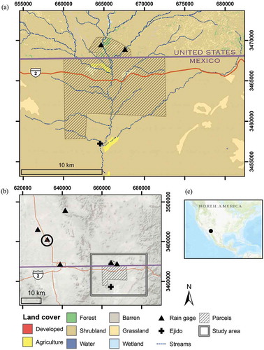
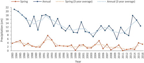
The vegetation of the San Bernardino Valley is predominately semi-desert grassland and desert scrub (Lowry et al. 2007) with riparian corridors of cottonwood-willow gallery forest, riparian grassland, and riparian shrubland (Malcom and Radke 2008). Cienegas develop along riparian corridors and join these more familiar riparian communities, where perennial water intersects the surface in channels sufficiently stable for biological succession to proceed (Hendrickson and Minckley 1984). The San Bernardino Valley is in the northwestern portion of the Chihuahuan Desert, where precipitation occurs primarily as rain in either late-summer monsoons or low-intensity winter storms and averaged 33 cm annually during the study period (1984–2016; Figure 2).

Figure 2. Extended spring (January–June, red) and annual (January–December, blue) precipitation based on monthly precipitation data from Douglas-Bisbee International Airport. Three year moving average shown with dotted lines.

Within the San Bernardino Valley, the U.S. Fish and Wildlife Service (FWS) San Bernardino National Wildlife Refuge (NWR) extends ~2.5 km north from the US–Mexico border; south of the border the Cuenca Los Ojos Foundation owns a large ranch, which runs along the Rio San Bernardino for ~7 km (Figure 3). Further south is the ‘18 de Agosto’ ejido. An ejido is a piece of land in Mexico, farmed communally under a system supported by the state and populated by multiple families who work there. The 18 de Agosto (Corral de Palos) ejido is located in the municipality of Agua Prieta, Sonora, Mexico. Most of the other land in the San Bernardino Valley consists of privately maintained large ranches.

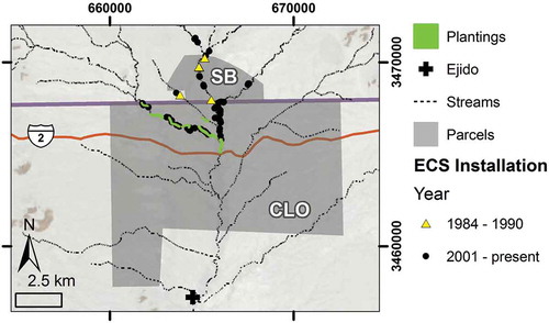
Figure 3. Spatiotemporal distribution of restoration. Several erosion control structures were installed from 1984 to 1991. No structures were installed from 1991 to 2000. Most structures were installed after 2001. Pole-planting occurred after 2007. San Bernardino National Wildlife Refuge (SB) is north of the international border, Cuenca Los Ojos ranch (CLO) is south of the border. Grazing was excluded from San Bernardino National Wildlife Refuge in 1984 and from Cuenca Los Ojos ranch in 2001. Basemaps by ESRI et al.; projection is WGS84 UTM 12N.

2.1. Restoration activities at Cienega San Bernardino

The San Bernardino NWR was created in 1980 (U.S. Fish and Wildlife Service 1979). In 2001, Cuenca Los Ojos ranch was acquired by the Cuenca Los Ojos Foundation for the purpose of environmental conservation. Both properties experienced extensive grazing, arroyo-cutting, and riparian habitats had been degraded prior to the current owners (L. Norman et al. 2014).

Restoration activities began at the San Bernardino NWR in 1980 with the removal of cattle, which is considered a passive restoration technique (Malcom and Radke 2008). Active restoration included both vegetative and watershed restoration. Undesired plants were eliminated or thinned, and desirable natives were planted. ECSs, specifically gabions, which are rock detention structures wrapped in wire, were installed in streams beginning in 1984 to reduce erosion and stabilize arroyos (L. Norman et al. 2014). Four ECSs were installed from 1984 to 1985 and one in 1990. There were no additional structures installed until 2002, when one ECS was installed by FWS. Five ECSs were installed between 2004 and 2005, two in 2008, and then seven from 2010 to 2012 (Figure 3). Of these 20 ECSs, FWS worked with local landowners to install four upstream of San Bernardino NWR northern boundary; the furthest is 1 km upstream (north) of San Bernardino NWR. Malcom and Radke (2008) found that passive restoration starting in 1980 resulted in the establishment of a riparian gallery over the course of 25 years that had not existed prior to the designation of San Bernardino NWR and new annual and emergent perennial vegetation was assisted by increased sediment deposition and greater availability of free-standing water within 2 years of construction of ECSs.

Restoration activities began on Cuenca Los Ojos ranch in 2001 with the removal of cattle as well as vegetative and watershed restoration. While grazing was excluded from the entire Cuenca Los Ojos property, most of the active restoration occurred between the International border and Route 2, which lies ~2.4 km south of the border in Sonora, Mexico (Figure 3). ECS installation began in 2001 and continues to this day (José Manuel Perez and Anna Valer Austin Clark, pers. comm.). Cuenca Los Ojos installed 49 large ECSs, gabions and earthen berms, between 2001 and 2017, 46 of which were documented using GPS in 2013 and form the basis of our analysis. In addition, more than 700 smaller loose-rock structures, called trincheras, and dirt plugs were installed. These smaller structures are not fully documented and not entirely constrained to the area north of Route 2. Where these small structures are documented, many occur in first-order streams (Strahler 1957), which were generally dry, upland drainages. Due to the lack of complete data, they were not included in the remote-sensing analysis, but results were examined for possible influence. Norman et al. (2014) found that biomass was re-established at the location of large ECSs in the Cienega San Bernardino despite drought conditions using NDVI over a 27 year period and field data over a 12 year period. Vegetative restoration has also occurred each year since 2007, with several hundred poles clipped from local cottonwood and willow trees and planted annually. These plantings occurred predominately in areas near the 46 documented ECSs north of Route 2; however, one section that was planted in 2015 extends 500 m south of Route 2.

ECS installation, as with any active restoration activity, constitutes a disturbance on the landscape. The magnitude of this disturbance depends on the type of ECS (gabion vs. one rock dam), requirements of construction (heavy machinery vs. hand crew), size of work crew, length of installation phase for individual ECSs, and rate of implementation (i.e. number of ECSs installed over a period of time). Many of these particulars are not recorded as part of Cuenca Los Ojos’s restoration project. However, rate of implementation is known for San Bernardino NWR ECSs and can be generalized for Cuenca Los Ojos ECSs. Installation periods for ECSs are visualized spatially and temporally (Figure 3).

3. Data and methods

Data preparation and analyses were performed using a combination of ESRI ArcGIS Desktop (ESRI 2016), Python (Python Software Foundation 2014), R (R Core Team 2017), and Microsoft Corporation (2013). R packages used include ggplot2 (Wickham 2009), Kendall (McLeod 2011), raster (Hijmans 2016), reshape (Wickham and Hadley 2007), rgdal (Bivand, Keitt, and Rowlingson 2017), and zoo (Zeileis and Grothendieck 2005).

3.1. Zone delineation

To investigate the extent that restoration impacts extend away from the restoration structures, the study area was classified into six zones based on proximity to ECSs and hydrologic characteristics (Figure 4). Large ECSs were documented using GPS by land managers at Cuenca Los Ojos and San Bernardino NWR as point locations in 2013 (L. Norman et al. 2014). Streamline data was derived from a high-resolution light detection and ranging data (Steven DeLong, pers. comm.) and National Elevation Data digital elevation model (10 m) classified according to Strahler stream order (Strahler 1957). First-order streams generally delineated upper watershed drainages with no riparian vegetation present and were removed from analysis. Due to the high resolution of the source data, areas of broad, flat topography, and other possible errors introduced during analysis, the resulting streams data set contained artifacts, such as streamlines not continuous with the larger stream complex and floodplains represented by multiple streamlines in one broad wash. These artifacts were compared to ESRI basemap imagery (0.3–1 m, ESRI et al. 2014) and corrected as needed. The riparian area was defined by buffering the linear stream data by 150 m to create a riparian area 300 m wide. Large ECS locations were then buffered by 300 m and the resulting areas clipped to the riparian area to define the

Figure 4. Definition of major and minor zones used to analyze spatial extent of restoration impacts. (a) Major zones were based on hydrologic relationship to ECSs. (b) Minor zones were subdivided into 1 km intervals. Upstream and downstream minor zones were based on distance to restoration. Tributary minor zones were based on distance from confluence with the Rio San Bernardino. Restoration, intra-restoration, and upland zones were not subdivided and are shown in gray (b). Projection is WGS84 UTM 12N.

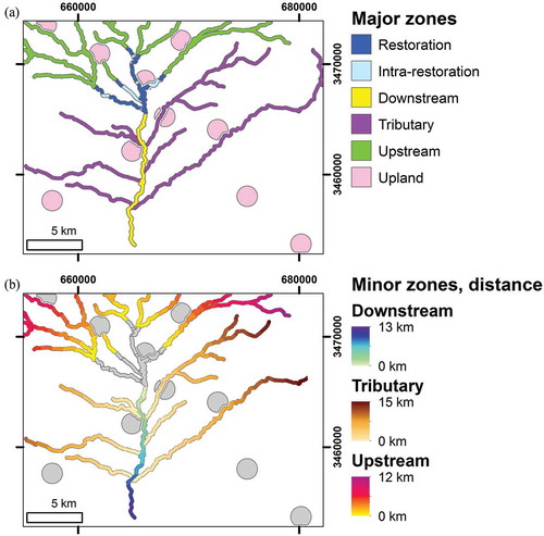
1. Restoration (treatment) zone: A 150 m corridor along a streamline area that extends 300 m upstream and downstream from an ECS.

Four other zones were developed to discern potential impacts of flow:

• (2) Intra-restoration: The riparian area between ECSs, which are more than 600 m apart.

• (3) Upstream: The riparian area upstream of the restoration zone. This extends to the end of the riparian area or to the edge of the study area.

• (4) Downstream: The riparian area downstream from the restoration zone, excluding any tributaries. This extends to the edge of the streams data.

• (5) Tributary: The riparian area of reaches that joined the downstream zone below the restoration zone.

To observe the general trend in the study area, an additional (6) upland zone was created (Wilson et al. 2016). To create the upland zone, 10 points were randomly distributed through the study area using ArcGIS Create Random Points tool. In order to approximately match the total area of the largest zone (the tributary zone; Table 1), the upland points were buffered by 927 m. This resulted in upland polygons that occasionally overlapped the riparian area. The riparian area, plus an additional 150 m buffer, was erased from the uplands area creating a separation between the upland zone and riparian areas. This prevents riparian and upland polygons from being adjacent; there is always a 150 m unassigned area between riparian and upland polygons (Figure 4).

Table 1. Area and pixel count for major zones in their entirety and subdivided into 1 km intervals for minor zone analysis.

Major zone		Minor zone
ID	Description	ID	Distance (km)	Area (ha)	Number of pixels
1	Restoration			450.26	4994
2	Intra-restoration			158.10	1762
3	Downstream			441.82	4913
		301	0–1	34.36	382
		302	1–2	39.07	435
		303	2–3	41.03	459
		304	3–4	36.10	397
		305	4–5	35.23	395
		306	5–6	32.47	361
		307	6–7	42.45	472
		308	7–8	38.25	430
		309	8–9	38.47	426
		310	9–10	35.11	388
		311	10–11	32.56	361
		312	11–12	35.30	392
		313	12–13	1.43	13
4	Tributary			2682.36	29,794
		401	0–1	266.39	2952
		402	1–2	304.58	3391
		403	2–3	237.01	2624
		404	3–4	198.16	2201
		405	4–5	187.04	2072
		406	5–6	263.53	2924
		407	6–7	196.12	2182
		408	7–8	148.11	1643
		409	8–9	151.23	1682
		410	9–10	110.38	1224
		411	10–11	105.42	1170
		412	11–12	113.71	1272
		413	12–13	87.28	970
		414	13–14	66.05	732
		415	14–15	44.56	495
5	Upstream			2192.49	24,394
		501	0–1	267.74	2980
		502	1–2	331.87	3703
		503	2–3	300.70	3335
		504	3–4	268.06	2980
		505	4–5	228.82	2537
		506	5–6	170.42	1894
		507	6–7	210.62	2336
		508	7–8	170.15	1895
		509	8–9	73.36	820
		510	9–10	81.26	907
		511	10–11	54.69	610
		512	11–12	34.81	386
6	Upland			2109.65	23,470

For upstream and downstream minor zones, distance refers to distance from restoration major zone. For tributary minor zones, distance refers to distance from confluence with main reach.

We hypothesize that restoration effects extend beyond the immediate restoration area, in the riparian corridor, based on hydrologic relationship to the ECSs. To test this, the major zones previously described were subdivided by distance from the restoration zone (Henshaw et al. 2013). These minor zones are defined by the Euclidean distance from the point of reference. Two separate intervals were used, 2.5 and 1 km. The intra-restoration zone was not subdivided because upstream and downstream restoration effects would be combined in the area, confounding the results. Additionally, the upland zone was not subdivided leaving only the three major zones to separate into minor zones (the upstream, downstream, and tributary zones).

Results from the minor zones delineated by 2.5 km intervals were comparable to those found in the minor zones delineated by 1 km intervals and the 1 km interval zones better describe the dynamics observed. Spatial data for major zones and minor zones delineated with 1 km intervals are available online (https://www.sciencebase.gov/catalog/item/5a2ecc42e4b08e6a89d3fbfb).

The upstream major zone was subdivided into minor zones based on distance upstream from the restoration zone. This resulted in 12 upstream minor zones, each one a 1 km interval. The downstream major zone was subdivided into minor zones based on distance downstream from the restoration zone. This resulted in 13 downstream minor zones. The tributary zone was subdivided based on distance upstream from the confluence of the tributary with the main reach and resulted in 15 tributary minor zones (Figure 4).

3.2. Climate data

Variations in climate, specifically in precipitation, affect the greenness and water content of aridland vegetation, and these effects need to be separated from those influenced by restoration activities. Similar to other aridlands, precipitation in the San Bernardino Valley is both spatial and temporally heterogeneous, making ground-based measurements invaluable. However, the area is also remote and straddles an international border; there are few weather stations near the study area in the US and no data was available from Mexico. Additionally, the study period spans decades, which presents another challenge in finding consistent climate data. The FWS installed weather stations on San Bernardino NWR in 2005, from which data was available until 2012. We compared this incomplete data with multiple data sets to find the most comprehensive and consistent data set. Ground station measurements from the National Climatic Data Center (NCDC, https://www.ncdc.noaa.gov/cdo-web/) were available for two stations for the period of interest, and interpolated (4 km resolution) monthly precipitation data was available from the PRISM Climate Group (http://www.prism.oregonstate.edu/, Daly et al. 2002). Data from the NCDC Douglas-Bisbee International Airport weather station, 35 km from San Bernardino NWR, was the most complete during the study period and closely correlated with the FWS stations for the 2005–2012 period (r = 0.82–0.92, p < 0.01). This station was the source of climate data for the analysis (Figures 1 and 2).

Previous studies of restoration at the Cienega San Bernardino used February to May to summarize precipitation for analysis (L. Norman et al. 2014), but recent research indicates that an extended spring season from January to June may be better suited to measure the impacts on the vegetation of precipitation-dependent habitats of southeastern Arizona and northeastern Sonora (Bodner and Robles 2017). This extended spring season was used to summarize precipitation for this research (Figure 2).

3.3. Satellite imagery

There are multiple satellite imagery data sets available for the area, varying in spatial and temporal resolution and the length of observation history. The Landsat program offers mid-resolution (30 m) data with one of the longest histories of earth observation. A combination of Landsat 5 TM and Landsat 8 Operational Land Imager (OLI) surface reflectance imagery was retrieved from USGS Earth Explorer. These satellites have a combined operational period of 1984 to the present, excluding 2012. While the Landsat 7 Enhanced Thematic Mapper Plus (ETM+) sensor was operational during 2012, an instrument failure in 2003 resulted in data not suitable for digital analysis. Because of this, we excluded the year 2012 from the 33 year study period of 1984 to 2016.

Landsat path/row (35/38) encompassed the study area. In this path/row, one scene per year was selected from the dry pre-monsoon summer season, April 15 to June 30. In this season, vegetation with access to surface and subsurface water will be most distinct from the otherwise dry and senescent landscape (Nguyen et al. 2015). Scenes were chosen based on the lack of clouds within the study area. If multiple cloud-free scenes were available for a particular year, the scene closest to early June was selected for analysis.

Although OLI and TM sensors have the same spatial resolution (30 m), there are slight differences in spectral resolution for the bands used in NDVI and NDII. There are not many direct comparisons of TM and OLI data but TM and ETM+ are considered complementary (Vogelmann et al. 2001; Martínez‐Beltrán et al. 2009; Claverie et al. 2015). The difference between OLI and ETM+/TM spectra is greater than between ETM+ and TM but surface reflectance is less affected by these systematic differences (Flood 2014). NDVI was demonstrated to be similar between OLI and ETM+ (Huntington et al. 2016) and OLI and ETM+ can be used as complementary data (Li, Jiang, and Feng 2013). This archive of TM, ETM+, OLI data, and specifically the surface reflectance products derived from these sensors, has been the basis of a variety of spatiotemporal ecological research (Guo and Gong 2016; Storey, Stow, and O’Leary 2016; Schaffer-Smith et al. 2017). These surface reflectance products form the basis of our analysis; the data is available from the U.S. Geological Survey through the Earth Explorer online interface (https://earthexplorer.usgs.gov/) and EPSA On-Demand System (http://espa.cr.usgs.gov).

3.4. Remote-sensing indices

Two remote-sensing indices were applied to Landsat data, NDVI and NDII. NDVI is a ratio combination of the visible red (red) and near-infrared (NIR) bands, centered at 0.660 and 0.840 µm, respectively, and indicates overall vegetation greenness or photosynthetically active vegetation (Equation (1); Jordan 1969; Rouse et al. 1974). NDII is a ratio combination of the NIR and shortwave infrared (SWIR) bands, centered at 0.840 and 1.676 µm, respectively, and indicates vegetation moisture content (Equation (2), Hardisky et al. 1984). Indices were applied to surface reflectance imagery.

(1) $\mathrm{N}\mathrm{D}\mathrm{V}\mathrm{I}=\frac{\left(\mathrm{N}\mathrm{I}\mathrm{R}-\mathrm{R}\mathrm{e}\mathrm{d}\right)}{\left(\mathrm{N}\mathrm{I}\mathrm{R}+\mathrm{R}\mathrm{e}\mathrm{d}\right)}$(1)

(2) $\mathrm{N}\mathrm{D}\mathrm{I}\mathrm{I}=\hspace{0.17em}\frac{\left(\mathrm{N}\mathrm{I}\mathrm{R}-\mathrm{S}\mathrm{W}\mathrm{I}\mathrm{R}\right)}{\left(\mathrm{N}\mathrm{I}\mathrm{R}+\mathrm{S}\mathrm{W}\mathrm{I}\mathrm{R}\right)}.$(2)

3.5. Analyses

3.5.1. Zonal trend analysis

To examine spatiotemporal changes in vegetation greenness and water content, a zone-based analysis was performed (Weiss et al. 2004; Wilson et al. 2016). For linear regression analysis, pixels were considered separate samples, resulting in high sample sizes (Table 1). The NDVI and NDII values for pixels in each major and minor zone were plotted over time and simple linear regression applied to determine the general empirical trend. Linear regression results in a simple linear model (Equation (3)), where m is the slope and b is the y-intercept. The slope (m) of the simple linear model was considered the general temporal trend. Temporal trends differ between zones, showing the spatial extent of restoration impacts as NDVI and NDII temporal trends change as the distance from restoration increases.

(3) $y=mx+b.$(3)

Simple linear regression allows for straightforward comparisons between areas (Fensholt et al. 2009) but it can be heavily affected by outliers (Chatterjee and Hadi 1986). To address this we also applied the nonparametric Mann–Kendall τ test for monotonic trends (Kendall 1938). The results of Mann–Kendall return a τ of −1 to 1. Results near 0 indicate little to no trend, while a τ closer to 1 or −1 indicate strong monotonic trends, positive or negative, respectively. Mann–Kendall is sensitive to the strength of the trend, and slight trends can be lost in the variability of the data (Yue, Pilon, and Cavadias 2002). Mann–Kendall required all pixel values in a zone be aggregated into a single value for analysis; mean NDVI and NDII were calculated for each zone per year and Mann–Kendall applied to the resulting time series for each zone. This lowered the effective sample size to one sample per zone per year.

3.5.2. Threshold area trend

Linear regression of NDVI and NDII values through time can indicate changes in vegetation, but another method to track vegetation changes is to apply a threshold to spectral index values to create binary rasters. Thresholds have been widely applied in this manner to track specific landscape characteristics (Otto, Scherer, and Richters 2011; Bertoldi, Drake, and Gurnell 2011; Henshaw et al. 2013). To track changes in the area of healthy vegetation within each zone, we performed a threshold-based zonal analysis. We determined a healthy vegetation threshold based on spectral index value means of areas of healthy vegetation delineated using Google Earth high-resolution imagery. We applied this threshold to spectral index values, calculated zonal statistics, and applied linear regression to examine the areal trend through time.

To determine the threshold, we examined Google Earth Pro (2016) imagery for a data set collected during the dry pre-monsoon summer season that was continuous for the entire study area. One set of imagery, collected on 7 June 2007, met that criteria. Based on this imagery, polygons were created in areas of dense and visually healthy cottonwood/willow forest and mesquite bosque in the riparian area. Polygons required areas of healthy vegetation large enough to capture multiple Landsat pixels. These green polygons were combined, resulting in 851 pixels defined as healthy vegetation; spatial data for green polygons are available online (https://www.sciencebase.gov/catalog/item/5a2ecc42e4b08e6a89d3fbfb). Descriptive statistics of NDVI and NDII values within the green polygons were calculated. By subtracting multiples of the standard deviation from the mean spectral index value (Table 2), several trial thresholds were developed. These trial thresholds were applied to the 2007 spectral index rasters. The resulting trial threshold rasters were compared to the original green polygons to determine the percentage of green polygon pixels correctly categorized by the trial threshold. Results of correctly categorized pixels combined with a visual analysis were used to determine the proper threshold for healthy vegetation. The ‘Number of Green Pixels’ refers to how many pixels of the 851 identified as healthy vegetation using aerial imagery were also identified as healthy vegetation using the threshold value applied to NDVI and NDII rasters (Table 2). NDVI and NDII thresholds were calculated separately but both were based on the same green polygons. For both NDVI and NDII, we determined the best threshold to be used in this analysis as two standard deviations below the mean index value.

Table 2. Development of trial thresholds for NDVI and NDII.

	NDVI			NDII
Formula	Threshold value	Number of green pixels	Proportion correct	Threshold value	Number of green pixels	Proportion correct
Mean	0.544	460	0.541	0.161	425	0.499
Mean – 1 SD	0.478	738	0.867	0.089	735	0.864
Mean – 2 SD	0.412	820	0.964	0.018	835	0.981
Mean – 3 SD	0.346	846	0.994	−0.054	847	0.995

Threshold value was determined by subtracting multiples of the standard deviation (SD) from the mean, shown in formulas. Number of green pixels is the number of pixels identified as green after application of the threshold value that are within the green polygon based on 2007 imagery. Proportion correct is the proportion of pixels identified by the threshold as green within the green polygon compared to the total number of pixels (851) within the green polygon.

These two thresholds were applied to the appropriate index rasters creating binary threshold rasters. Calculation of zonal statistics, specifically zonal mean, of the binary threshold rasters returns the percent of a zone above the threshold, our metric for proportion of healthy vegetation within a zone. The trend through time of this proportion of healthy vegetation in a zone was calculated by linear regression.

3.5.3. Short-term temporal pattern analysis

The generalized temporal trends described by linear regression of NDVI and NDII values and linear regression of threshold raster may obscure short-term temporal patterns, which could clarify the relationship between restoration activity and landscape response. To examine these short-term temporal patterns and their spatial relationship to restoration, we plotted NDVI and NDII means for each zone over time. To reduce interannual variability, we added a series smoothed by a moving average with a 3 year unweighted window (Suppiah and Hennessy 1998; De Luı́s et al. 2001). Short-term temporal patterns were described, then compared between major and minor zones.

3.5.4. Precipitation correlation analysis

In our study area, vegetation greenness and water content are highly affected by precipitation and this variability could obscure the effects of restoration techniques (Nemani et al. 2003). To clarify the relationship between precipitation and vegetation, and explore the effects of ECSs on that relationship, we examined the correlation between spring precipitation and NDVI/NDII values. Pearson’s product–moment correlation (r) was calculated between precipitation and spectral index values for each major and minor zone.

4. Results

4.1. Zonal trend analysis

4.1.1. Linear regression

Linear regression was used to generalize the temporal trend in NDVI and NDII values for each major and minor zone. The scales of NDVI and NDII, while theoretically being −1 to 1, are, in this region, much more constrained; when changes in NDVI and NDII are regressed against the scale of decades (1984–2016), it creates trend values that seem small but are consistent with the magnitude of other results reported in the literature (Fensholt et al. 2009; L. Norman et al. 2014; Nguyen et al. 2015). Evaluation of trend intensity was data driven based on relative slope (m) values of the individual analyses. A trend within ½ standard deviation from m = 0 was considered to be very slight and indicate little to no change overall, ½ to 1½ standard deviations from m = 0 was considered a minor trend, moderate trends extended from 1½ to 2½ standard deviations, and strong trends were greater than 2½ standard deviations from m = 0. Pixels were evaluated as separate samples and the resulting sample sizes resulted in high significance for most findings; unless otherwise stated p < 0.01 for the results in this section.

When evaluating the major zones (Figure 5), the temporal trend showed the strongest increases in the restoration zone for both spectral indices, though the magnitude of this increase was minor. The intra-restoration zone showed a very slight decrease in NDVI values and a minor decrease in NDII values. The downstream zone saw a very slight increase in NDVI values, while NDII showed a minor decrease. NDVI values for the tributary, upstream, and upland zones showed a moderate decrease with the upland zone seeing the strongest negative trend. NDII values showed a very slight decrease in the upstream zone and moderate decreases in the tributary and upland zones with tributary showing the strongest negative trend.

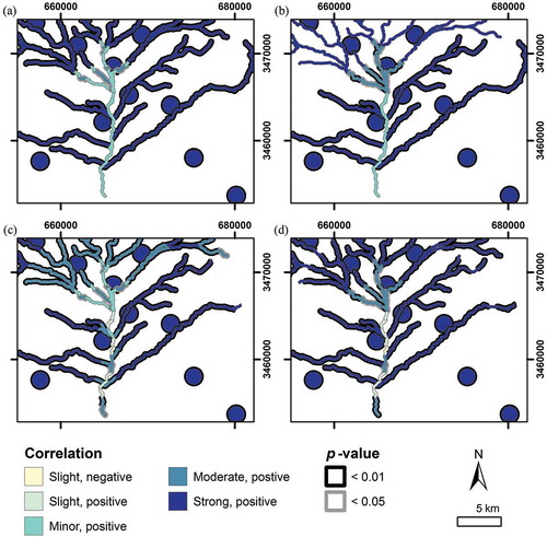
Figure 5. Results of linear regression of NDVI and NDII showing the strength of temporal trend in vegetation greenness and water content. Slope of the regression (m) represents the strength of the temporal trend and is signified by color, p values are signified by the border. (a) Major zone NDII trend. (b) Major zone NDVI trend. (c) Minor zone NDII trend. (d) Minor zone NDVI trend. Projection is WGS84 UTM 12N.

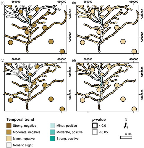
In the minor zones (Figure 5), trends in the tributary minor zones are minor to moderate and negative for both indices, with NDII being generally more negative than NDVI. Neither shows a clear spatial pattern. In the upstream minor zones, there is a difference between indices. NDVI trends show little to no trend 0 to 2 km upstream of the restoration zone; beyond 2 km upstream NDVI trends are slightly to moderately negative, matching tributary zones. However, NDII trends in the upstream zones are neutral 0 to 6 km upstream from restoration; beyond 6 km upstream NDII trends are slightly to moderately negative matching the NDII trends found in the tributary zones.

In downstream minor zones, both indices present a similar pattern (Figure 6). From 0 to 5 km downstream from restoration, trends are more positive (NDVI) or less negative (NDII) than those seen in upland and tributary minor zones. At 5 to 6 km downstream, the trends decrease to match those seen in upland and tributary zones.. From 6 to 10 km downstream of restoration, trends increase as the reach nears the ejido. At 10 km and further downstream the NDII trends again align with those in the upstream and tributary zones while NDVI trends are more negative than those in the upstream and tributary zones.

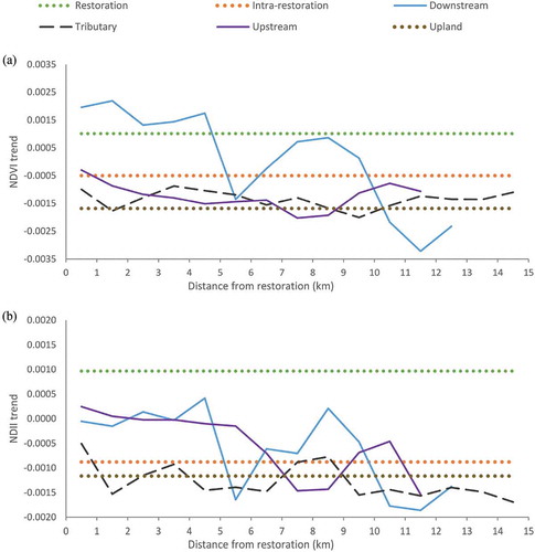
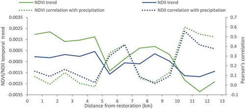
Figure 6. Trends in vegetation greenness and water content change based on distance from restoration. (a) NDVI and (b) NDII trends are higher in restored areas, areas 0–5 km downstream of restoration, and near the ejido, 6–10 km downstream. NDII trends are also high 0–6 km upstream of restoration. For upstream and downstream zones (solid lines), x-axis indicates distance (km) from restoration zone. For tributaries (dashed line), x-axis indicates distance (km) from confluence with main reach. Restoration, intra-restoration, and upland (dotted lines) were not subdivided into minor zones; the trends for these zones are shown as horizontal lines.

4.1.2. Mann–Kendall test

Mann–Kendall does not test for general trend but rather for the monotonicity of the trend: are the changes between time samples (years) increasing or decreasing? In this section, when referring to a trend’s intensity (slight, weak, moderate, strong), we are referring to the monotonicity of the trend. Generally, Mann–Kendall applied to NDII values display trends that are more negative and inconclusive compared to NDVI trends.

When evaluating the major zones (Figure 7), the restoration zone NDVI trend was slightly positive and NDII trend was weakly positive but neither was significant. The intra-restoration zone was weakly negative for both NDVI and NDII but with no significance. The NDVI trend in the downstream major zone was slightly positive while the NDII trend was weakly negative but neither were significant. Tributary trends were weakly negative for NDVI values and moderately negative for NDII values. Upstream major zone trends were weakly negative for NDVI values and weakly negative and insignificant for NDII values. Upland zone trends were moderately negative for NDVI values and weakly negative for NDII values.

Figure 7. Results of Mann–Kendall test applied to NDVI and NDII showing the monotonicity of the temporal trend in vegetation greenness and water content. The degree of monotonicity (τ) is signified by color, p values are signified by the border. (a) Major zone NDII trend. (b) Major zone NDVI trend. (c) Minor zone NDII trend. (d) Minor zone NDVI trend. Projection is WGS84 UTM 12N.

When evaluating the minor zones, tributary minor zones for both indices are weakly to moderately monotonic and negative with no clear spatial pattern. Upstream minor zones for NDVI show generally weak and moderate monotonic and negative trends except for 0 to 1 km upstream and further than 10 km. Upstream minor zones are less conclusive for NDII trends, displaying no clear trend until 7 km upstream of restoration. From 7 to 9 km upstream, NDII trends show moderate monotonic and negative trends. From 9 to 11 km, trends are less conclusive before returning to a moderate negative trend at 11 km.

In downstream minor zones from 0 to 5 km, NDVI trends are weakly to moderately monotonic and positive while NDII trends are inconclusive. From 5 to 6 km, the NDVI downstream trend becomes negative and inconclusive while the NDII trend becomes negative and significant. The ejido confounds both analyses from 6 to 10 km from NDVI and 6 to 9 km for NDII. Downstream of the ejido, further than 10 km for NDVI and 9 km for NDII, trends for both indices are significant, weakly to moderately monotonic, and negative.

4.2. Threshold area analysis

The healthy vegetation threshold analysis tracks the changes in proportion of healthy vegetation in each major and minor zone through the study period. This analysis aggregates pixels to a single proportional value for each zone that limits the sample size of the analysis; effectively there is one sample per zone per year that reduces statistical power.

When evaluating the major zones (Figure 8), the temporal trend showed the strongest increases in the restoration zone for both spectral indices; the magnitude of this increase for NDVI was moderate and significant while NDII was minor and insignificant. The trends in the intra-restoration zone for both NDVI and NDII were very slight and not statistically significant. The trend for the downstream major zone is minor for both NDVI and NDII though NDVI is positive and NDII is negative; neither trends were significant. Trends for tributary, upstream, and upland major zones, were not significant for the proportion based on the NDVI threshold. For the proportion based on the NDII threshold, trends for upstream and upland major zones were slightly negative and significant. The tributary zone was not significant for NDII. Since the tributary, upstream, and upland zones had little areas of healthy vegetation at the start of the study period, trends in areal proportion in these zones could not be strongly negative since the trend was bounded by a lower limit of 0% healthy vegetation.

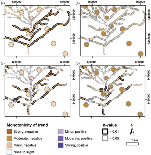
Figure 8. Results showing the temporal trend in areal proportion of healthy vegetation as determined by application of threshold to NDVI and NDII rasters. Positive trends indicate an increase in healthy vegetation area in a zone, and negative trends indicate a loss of healthy vegetation in a zone. Slope of the regression (m) represents the strength of the temporal trend and is signified by color, p values are signified by the border. (a) Major zone NDII trend. (b) Major zone NDVI trend. (c) Minor zone NDII trend. (d) Minor zone NDVI trend. Projection is WGS84 UTM 12N.

In the upstream minor zones, there is a difference between threshold-based trends. NDVI-based trends show a minor positive trend 0 to 1 km upstream of restoration; beyond 1 km trends are neutral, varying between slightly positive or negative but with no significance, which is similar to trends found in the tributary minor zones. However, NDII-based trends in the upstream zones are neutral 0 to 6 km upstream from the restoration zone; beyond 6 km trends are slightly to moderately negative matching the trends found in NDII-based threshold values in tributary zones.

In downstream minor zones, both indices present a similar pattern though NDII-based trends are more negative than NDVI-based trends. From 0 to 5 km downstream from restoration, trends are positive or much less negative than those seen in upland and tributary zones. At 5 to 6 km downstream, the trends decrease sharply and, in contrast to the pattern displayed in the zonal analysis, at 5 to 6 km the negative trend in this threshold-based analysis exceeds the trends in the tributary and upland zones. Downstream 6 to 10 km from restoration, trends increase as the reach nears the ejido. At 10 km and further downstream both NDII and NDVI trends become negative and exceed the magnitude of trends in tributary or upland zones. This is not unexpected as the downstream minor zones had significant areas of healthy vegetation, which they could lose while the tributary and upland zones did not.

4.3. Short-term temporal pattern analysis

When examining short-term temporal patterns in the major zones, two distinct patterns emerge (Figure 9). One pattern displays a trough at 1990 followed by a peak in 1992 and a decline after 1992. This corresponds to a general decline in spring and annual precipitation from 1984 to 1990 followed by unusually high rainfall from 1991 to 1993 and subsequent decline until 1999 (Figure 2). This trough–peak–decline (1990–1995) pattern is present in NDVI and NDII values for restoration and intra-restoration major zones, though it is less distinct for NDII values. This pattern persists but is less distinct for NDVI values in the downstream major zone. For NDII values in the downstream major zone, this pattern is almost nonexistent. For both NDVI and NDII values, the pattern exists in tributary, upstream, and upland major zones. The NDII patterns are less distinct than patterns in NDVI values for these zones but more distinct than NDII patterns for the restoration and intra-restoration zones. For NDVI, this pattern is most prominent in the upstream major zone.

Figure 9. Results of short-term pattern analysis for major zones. Index mean values were charted over time for each major zone, linear trend, and 3 year moving average are included. NDVI is green with overall higher values, NDII is blue and has lower values. Gray bars at top indicate the trough–peak–decline pattern from 1990 to 1995 and the rough sinusoidal curve from 1999 to 2013.

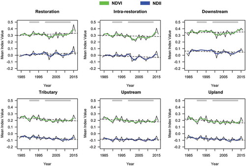
The other pattern in the major zones is a roughly sinusoidal curve beginning at 1999. Values decline from 1999 to 2003, then increase until a peak in 2006, decrease again from 2006 to 2010, and then increasing until at least 2013. Spring precipitation is generally constant during this period, though annual precipitation shows a peak in 2007 and increase after 2011. This pattern is more variable between zones and indices than the trough–peak–decline pattern. For NDVI, this pattern is present in the restoration, intra-restoration, and downstream major zones. For these zones, the initial trough in 2003 is greater than in 2010. In the downstream major zone, the pattern is present but the least distinct with the 2010 trough relatively shallow. In NDII values, this rough sine pattern is also present in restoration, intra-restoration, and downstream major zones and more distinct than in NDVI. For NDII, the 2010 trough is more pronounced than NDVI, being almost equal to the 2003 trough in each zone. Similar to NDVI, the downstream major zone had a relatively less distinct pattern compared to restoration and intra-restoration zones. For both NDVI and NDII, in the tributary, upstream, and upland major zones, this pattern disappears. For these zones, NDVI values from 1999 to 2013 display slight variations around a gentle trough below the general trend for the zone. NDII values for that same period show the same slight variations but follow the general trend for the zone.

The tributary and upstream minor zones and the upland major zone for both NDVI and NDII display the trough–peak–decline pattern from 1990 to 1995 and lack the rough sine pattern from 1999 to 2013. For both indices, the trough–peak–decline pattern is less prominent and the rough sine pattern emerges in the restoration and intra-restoration zones. There are differences between indices in the downstream minor zones. For NDVI, the trough–peak–decline pattern is present in most downstream minor zones but becomes a trough–peak–increase/steady pattern from 0 to 3 km and 6 to 7 km downstream from restoration. For NDII, the trough–peak–decline pattern is not present in any zones but instead a rise–steady pattern emerges for the periods of 1985 to 1999. This rise–steady pattern is present from 0 to 5 km downstream; at 5 to 6 km the pattern changes to a rise–decline. From 6 to 10 km downstream, the rise–steady pattern of NDII values re-emerges before disappearing further than 10 km from restoration. In the downstream minor zones, NDVI and NDII display a similar spatial distribution of the rough sine temporal pattern. The sine pattern is present 0 to 5 km downstream of restoration. From 5 to 6 km downstream, the pattern disappears. Downstream 6 to 7 km from restoration, in NDII the rough sine reappears though the second trough is delayed but the pattern remains absent in NDVI values. From 7 to 10 km, the rough sine pattern is apparent in both NDVI and NDII before disappearing in both further than 10 km downstream from restoration.

4.4. Precipitation correlation analysis

Spring precipitation was also analyzed for general temporal trend using linear regression and monotonicity of trend using Mann–Kendall. Linear regression results indicated a moderately negative trend (m = −0.0743, p = 0.015) with minor monotonicity (τ = −0.25, p = 0.042) in spring precipitation. This allows us to contextualize the results from Pearson’s product–moment correlations between NDVI and NDII and spring precipitation.

When evaluating NDVI values in major zones (Figure 10), the tributary, upstream, and upland major zones were similarly and strongly correlated to spring precipitation. NDII values were also strongly correlated with spring precipitation in the tributary, upstream, and upland major zones. Of NDVI correlations, the downstream major zone had the lowest correlation with spring precipitation; the weak correlation was not significant. Similarly, in NDII correlations, the downstream major zone had the lowest correlation with spring precipitation and the weak correlation was not significant. NDVI values in the restoration and intra-restoration zones were moderately correlated with spring precipitation. NDII values in the restoration zone were weakly correlated with spring precipitation but not significantly, while the intra-restoration zone showed a moderate correlation.

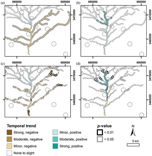
Figure 10. Correlation of NDVI and NDII values with spring precipitation. Areas restored and downstream of restoration are less correlated with precipitation. Pearson’s R represents the strength of the correlation and is signified by color, p values are signified by the border. (a) Major zone NDII trend. (b) Major zone NDVI trend. (c) Minor zone NDII trend. (d) Minor zone NDVI trend. Projection is WGS84 UTM 12N.

Overall, in the minor zones, NDVI and NDII display the same spatial pattern in correlations with spring precipitation, though NDII correlations are generally slightly lower. Tributary, upstream, and upland zone spectral values are highly correlated with spring precipitation. Tributary and upstream minor zones show no spatial pattern in correlations. Restoration and intra-restoration zone NDVI and NDII values are moderately correlated with spring precipitation. Downstream minor zones from 0 to 5 km are not correlated. From 5 to 6 km, the correlation may be more moderate but this finding lacks significance. From 6 to 7 km downstream, there is a significant finding of moderate correlation with precipitation for both NDVI and NDII values. From 7 to 10 km downstream of restoration, correlations become insignificant as the reach passes through the ejido. Beyond 10 km downstream, both NDVI and NDII values become moderately correlated with precipitation though not as strongly as tributary, upstream, and upland zones.

This spatial pattern of precipitation correlations is inverse that of zonal trend and threshold area analysis (Figure 11).

Figure 11. Spatial pattern of correlation with spring precipitation compared to linear regression derived temporal trends for vegetation greenness and water content. Correlation with precipitation shown with dotted lines, and linear regression slope (m) derived temporal trends shown with solid lines; NDVI is shown in green, and NDII is shown in blue. Temporal trends in NDVI and NDII are higher and decoupled from precipitation in areas closer to restoration and in the area surrounding the ejido (6–10 km).

5. Discussion

Analyses had marked differences in statistical power. In the zonal trend analysis and correlation analysis, pixels were treated as independent samples, resulting in very large sample sizes (Table 1). Pixels are not truly independent due to spatial autocorrelation. This inflated sample size increases the likelihood of statistical significance without corresponding practical significance (Yue, Pilon, and Cavadias 2002). The threshold area analysis and the Mann–Kendall test limit the sample size of the analysis to one sample per zone per year, and this low sample size decreases the likelihood of statistical significance. By comparing these approaches and evaluating patterns common to both, we can temper our conclusions, avoiding the perils of both under- and overconfidence.

Trends in NDVI, which measures vegetation greenness, were generally more positive than trends in NDII, which measures vegetation canopy moisture. This may be due to the interactions of soil moisture and canopy cover, canopy health on the indices. Malcom and Radke (2008) noted the increase in tree cover due to passive restoration on San Bernardino NWR and the development of favorable conditions to tree establishment shortly after ECS installation. As canopy cover increases, either due to vegetation community shifts or from increased vegetation health, soil reflectance decreases as it becomes overtopped by canopy reflectance. NDVI is negatively affected by soil moisture but is very responsive to canopy cover (Carlson, Gillies, and Perry 1994; Carlson and Ripley 1997; P. L. Nagler, Glenn, and Huete 2001), whereas NDII is positively affected by soil moisture as well as canopy moisture (Hunt and Yilmaz 2007). As canopy cover increased, the loss of soil moisture reflectance was not equally matched by increased canopy water content during the dry summer season, resulting in lower NDII values. NDVI, however, reacted to both increase in canopy cover and reduction of the adverse effects of soil moisture on index values. Examining vegetation–moisture trends across all seasons may clarify the effects of ECSs on vegetation moisture.

For all long-term trend analyses, linear regression of NDVI and NDII values, changes in area of healthy vegetation, and monotonic trend tests, the restoration zone had the highest positive trends of the major zones for both indices. However, this was often matched and exceeded in the downstream minor zones for NDVI. Within the downstream zones, trends were highest from 0 to 5 km downstream of the restoration zone for all trend analyses. NDVI trends tended to be positive and significant while NDII values tended to be neutral and insignificant. At 5 km downstream, there was a distinct change and trends became negative: either minor, negative, and insignificant for NDVI or more strongly negative and significant for NDII. This could mark the boundary of influence of ECSs, but it also occurs at the edge of the Cuenca Los Ojos property. Cuenca Los Ojos ranch ends between 4 and 5 km downstream of restoration, and cattle are excluded from the entire property. Given the magnitude of the change from 5 to 6 km downstream of restoration and the lack of similar change in cattle-excluded tributaries or upland areas, these results are likely a combination of the impacts of ECSs and cattle exclusion. Consistent throughout analyses was the confounding effect of the ejido and surrounding farmlands. The ejido occurs between 8 and 9 km downstream of the restoration zone and consists of a small residential area on the west side of the riparian corridor and a large field between the main riparian corridor and a tributary drainage. The effects of the ejido extended either from 6 or 7 km, dependent on analysis, down to 10 km downstream of restoration. Trends in the area are generally more stable or increasing relative to zones further downstream or when compared to upstream and tributary zones. Agricultural land use requires adequate levels of water and vegetation production for field crops or cattle; the water may be diverted from the main reach or pumped from groundwater sources to maintain vegetation trends in this area. It is possible that the trends in the area of the ejido would be similar if no restoration occurred upstream. Therefore, it is unclear to what extent the effects of the ejido interact with the effects of the upstream restoration and the groundwater systems. At 10 km downstream and further, trend analyses for both indices displayed values similar to tributary and upland zones, which may indicate a definitive downstream boundary in restoration effects.

Upstream zones were expected to be similar to tributary zones. Departures from that similarity, marked by higher positive trends (NDVI) or less negative trends (NDII) immediately upstream of the restoration zone, indicate the influence of ECSs extend upstream as well as downstream. Indices differed in the spatial extent of that influence. NDVI-based analyses showed restoration effects only immediately upstream of the restoration zone, 0 to 1 km, while NDII-based analyses showed effects as far as 4 to 6 km upstream of the restoration zone. These effects, however, were less consistently significant through the three long-term trend analyses. This may indicate that any upstream effects present may be more subtle and delayed compared to downstream effects, or upstream impacts may be attenuated by cattle, as grazing is likely continuing upstream and outside the borders of San Bernardino NWR and Cuenca Los Ojos ranch. The further extent of affected NDII values may indicate that NDII can identify changes better in canopies under grazing pressure or that changes in canopy water, though generally of a lower magnitude than changes in greenness, may precede changes in greenness. The presence of impacts upstream, despite the high probability of continued grazing pressure, indicates that investigation into hydrologic effects of ECSs may be warranted further upstream than previously examined.

Analysis of the correlation to precipitation in a landscape with vegetation dynamics primarily driven by precipitation (Nemani et al. 2003) can reveal changes caused by restoration and other anthropogenic factors. Spatial patterns mirror the trend analysis, with downstream zones closer to restoration, 0 to 5 km, being least correlated with precipitation for both NDVI and NDII and downstream zones beyond 10 km being more correlated with precipitation. The ejido again complicated our analyses at the region from 7 to 10 km downstream of restoration. Over the study period spring precipitation decreased, thus areas with positive trends in vegetation metrics are expected to be less correlated. In these areas, where vegetation metrics are decoupled from precipitation, water must be available in some form to supplement the lack of precipitation. Future research would be improved by using techniques developed to definitively separate anthropogenic effects from interannual precipitation variability (Evans and Geerken 2004; Verbesselt et al. 2010; Burrell, Evans, and Liu 2017). Additionally, this could clarify whether restoration efforts are improving land health or merely preventing further degradation.

Short-term temporal patterns give insight into possible causes for this decoupling of precipitation and vegetation response. The trough–peak–decline pattern of 1990 to 1995 is common to both NDVI and NDII values and follows changes in precipitation for that period. The pattern is strongest in tributary, upstream, and upland zones. In the restoration zone, this precipitation driven pattern is nonexistent in NDII values and diminished in NDVI. In downstream zones, this pattern disappears in NDII and is replaced by a rise–steady pattern from 1986 to 1999, decoupling NDII values from precipitation. For NDVI values, the trough–peak decline is modified to a trough–peak–increase/steady pattern, which matches short-term changes in precipitation but without following the overall trend of decreasing spring precipitation. This indicates that ECSs have increased water availability in those zones, allowing vegetation to be less dependent on precipitation, which is observable in vegetation response.

The other short-term temporal pattern evident, the rough sine pattern from 1999 to 2013 is present only in restoration, intra-restoration, and downstream zones. This pattern, in combination with the long-term trends, drives the lower correlation with precipitation for those zones. In downstream zones for both NDVI and NDII, it is more distinct within 5 km of the restoration zone. This pattern begins with a decline in 1999, two years before Cuenca Los Ojos began restoration efforts but concurrent with a slight drop in spring precipitation and lower levels of annual precipitation. It then departs from both precipitation trends and the long-term trend of the individual zones, which indicates acute anthropogenic effects during this period. This pattern disappeared from 5 to 7 km downstream of restoration. In the region of the ejido, 7 to 10 km downstream, a weaker rough sine pattern re-emerges. This cannot be explained solely by local agricultural land-use practices and indicates interactions between the effects of upstream restoration and local effects from the ejido. Further than 10 km from restoration, and downstream of the ejido, the rough sine pattern disappears, which matches the definitive boundary for restoration effects found in long-term trends.

The sine pattern is present only in restoration, intra-restoration, and downstream major zones, and it is more pronounced in downstream subdivided zones that are closer to the restoration zone, matching spatial pattern of other restoration effects. Therefore, the rough sine pattern is likely linked to restoration activities. The shape of this pattern points to possible variations in ECSs’ implementation rates. The lack of precise dates for ECS implementation precludes definitive associations but ECS implementation was likely not consistent through the study period and the sine pattern suggests two separate surges of ECS construction. If so, the swiftness with which the troughs of the sine pattern regain a level approximating the long-term trend then indicates the recovery of the landscape from restoration implementation disturbance. The downstream zones closest to the restoration zone, 0 to 2 km, have the strongest sine pattern for both indices, and in these zones, NDVI and NDII values approximate the long-term trend line 2 to 4 years after the initial disturbance of restoration.

6. Conclusion

By using both NDVI and NDII, and a variety of statistical approaches, a more detailed account of the spatial and temporal effects of restoration was described. Neither NDVI nor NDII was ‘better’ than the other; instead, they highlighted different vegetation–water dynamics, which improved analysis compared to a single index study. Restoration effects observed include increases in vegetation greenness captured by NDVI, increased or steady vegetation water content captured by NDII, and a decoupling of greenness and vegetation water content from seasonal precipitation. Despite the relative long period of the Landsat archive, there is no true ‘pre-restoration’ data available for trend analysis at this location. As remote-sensing platforms continue to mature and new restoration projects develop, there will be more opportunities for pre-restoration, during restoration, and post-restoration trend analysis on a decadal scale.

We found that over a 33 year period the positive impacts of active restoration on vegetation health extend beyond the immediate area of restoration activities and combine with passive restoration management techniques. While active restoration techniques such as invasive plant removal and pole planting may have local, temporary effects on NDVI, long-term and nonlocal effects require modification of underlying ecological processes that support vegetation growth. Additionally, techniques such as invasive removal and prescribed burns could decrease greenness and vegetation water content initially; any trends in NDVI or NDII affected by restoration should be assessed with an understanding of the purpose of particular restoration techniques, the communities being affected and the underlying ecology processes of the region. In our study area, we found that the installation of ECSs initially resulted in negative effects at the site of restoration and downstream, presumably because of the disturbance of construction and initial retention of flow. However, these effects disappeared within 2 to 4 years as NDVI and NDII rebounded, indicating a change in the underlying hydrology of the riparian corridor, which in turn affected the corridor vegetation. Strong effects, such as positive greenness trends that counter the negative trends found in tributaries and upland zones, extend approximately 5 km downstream from restoration sites. These effects dwindle beyond 10 km downstream as greenness trends, moisture trends, and correlation with seasonal precipitation align with those seen in upstream, tributary, and upland zones. It is important for water policymakers and restoration practitioners to understand that the installation of ECSs at desert cienegas might not decrease water availability downstream, but instead can provide long-term water-storage opportunities that riparian obligates could harvest over time. Our research defines this extrapolation to extend ~5 km downstream from restoration to the benefit of the Rio Yaqui watershed.

Acknowledgments

This research was conducted with support from the Land Change Science (LCS) Program under the Land Resources Mission Area of the U.S. Geological Survey. Many thanks to Bill Radke of the USFWS as well as Anna Valer Austin Clark and José Manuel Perez of Cuenca Los Ojos for sharing their knowledge of and commitment to the Cienega San Bernardino watershed. We appreciate the peer reviews done by Drs. Pamela Nagler and Jessica Walker, USGS. Any use of trade, firm, or product names is for descriptive purposes only and does not imply endorsement by the U.S. government.

Disclosure statement

No potential conflict of interest was reported by the authors.

References

- Adam, E., O. Mutanga, and D. Rugege. 2010. “Multispectral and Hyperspectral Remote Sensing for Identification and Mapping of Wetland Vegetation: A Review.” Wetlands Ecology and Management 18 (3): 281–296. doi:10.1007/s11273-009-9169-z.
- Aguilar, C., J. C. Zinnert, M. J. Polo, and D. R. Young. 2012. “NDVI as an Indicator for Changes in Water Availability to Woody Vegetation.” Ecological Indicators 23 (December): 290–300. doi:10.1016/j.ecolind.2012.04.008.
- Bertoldi, W., N. A. Drake, and A. M. Gurnell. 2011. “Interactions between River Flows and Colonizing Vegetation on a Braided River: Exploring Spatial and Temporal Dynamics in Riparian Vegetation Cover Using Satellite Data.” Earth Surface Processes and Landforms 36 (11): 1474–1486. doi:10.1002/esp.v36.11.
- Biggs, T. H., R. S. Leighty, S. J. Skotnicki, and P. A. Pearthree. 1999. Geology and Geomorphology of the San Bernardino Valley, Southeastern Arizona. Tucson, AZ: Arizona Geological Survey.
- Bivand, R., T. Keitt, and B. Rowlingson. 2017. “Rgdal: Bindings for the Geospatial Data Abstraction Library.” https://CRAN.R-project.org/package=rgdal.
- Bodner, G. S., and M. D. Robles. 2017. “Enduring a Decade of Drought: Patterns and Drivers of Vegetation Change in a Semi-Arid Grassland.” Journal of Arid Environments 136 (January): 1–14. doi:10.1016/j.jaridenv.2016.09.002.
- Bruce, J. K., C. E. Edmonds, E. Terrance Slonecker, J. D. Wickham, A. C. Neale, T. G. Wade, K. H. Riitters, and W. G. Kepner. 2008. “Detecting Changes in Riparian Habitat Conditions Based on Patterns of Greenness Change: A Case Study from the Upper San Pedro River Basin, USA.” Ecological Indicators 8 (1): 89–99. doi:10.1016/j.ecolind.2007.01.001.
- Burrell, A. L., J. P. Evans, and Y. Liu. 2017. “Detecting Dryland Degradation Using Time Series Segmentation and Residual Trend Analysis (TSS-RESTREND).” Remote Sensing of Environment 197 (Supplement C): 43–57. doi:10.1016/j.rse.2017.05.018.
- Carlson, T. N., and D. A. Ripley. 1997. “On the Relation between NDVI, Fractional Vegetation Cover, and Leaf Area Index.” Remote Sensing of Environment 62 (3): 241–252. doi:10.1016/S0034-4257(97)00104-1.
- Carlson, T. N., R. R. Gillies, and E. M. Perry. 1994. “A Method to Make Use of Thermal Infrared Temperature and NDVI Measurements to Infer Surface Soil Water Content and Fractional Vegetation Cover.” Remote Sensing Reviews 9 (1–2): 161–173. doi:10.1080/02757259409532220.
- Caves, J. K., G. S. Bodner, K. Simms, L. A. Fisher, and T. Robertson. 2013. “Integrating Collaboration, Adaptive Management, and Scenario-Planning: Experiences at Las Cienegas National Conservation Area.” Ecology and Society 18 (3): 43. doi:10.5751/ES-05749-180343.
- Chatterjee, S., and A. S. Hadi. 1986. “Influential Observations, High Leverage Points, and Outliers in Linear Regression.” Statistical Science 1 (3): 379–393. doi:10.1214/ss/1177013622.
- Chuvieco, E., D. Riaño, I. Aguado, and D. Cocero. 2002. “Estimation of Fuel Moisture Content from Multitemporal Analysis of Landsat Thematic Mapper Reflectance Data: Applications in Fire Danger Assessment.” International Journal of Remote Sensing 23 (11): 2145–2162. doi:10.1080/01431160110069818.
- Claverie, M., E. F. Vermote, B. Franch, and J. G. Masek. 2015. “Evaluation of the Landsat-5 TM and Landsat-7 ETM + Surface Reflectance Products.” Remote Sensing of Environment 169 (November): 390–403. doi:10.1016/j.rse.2015.08.030.
- Daly, C., W. P. Gibson, G. H. Taylor, G. L. Johnson, and P. Pasteris. 2002. “A Knowledge-Based Approach to the Statistical Mapping of Climate.” Climate Research 22 (2): 99–113. doi:10.3354/cr022099.
- ESRI. 2016. ArcGIS Desktop (Version 10.5). Redlands, CA: ESRI.
- ESRI, DigitalGlobe, GeoEye, Earthstar Geographics, CNES/Airbus DS, USDA, USGS, AeroGRID, IGN, and GIS User Community. 2014. World Imagery. Basemaps. Redlands, CA: ESRI.
- Evans, J., and R. Geerken. 2004. “Discrimination between Climate and Human-Induced Dryland Degradation.” Journal of Arid Environments 57 (4): 535–554. doi:10.1016/S0140-1963(03)00121-6.
- Fensholt, R., K. Rasmussen, T. T. Nielsen, and C. Mbow. 2009. “Evaluation of Earth Observation Based Long Term Vegetation Trends — Intercomparing NDVI Time Series Trend Analysis Consistency of Sahel from AVHRR GIMMS, Terra MODIS and SPOT VGT Data.” Remote Sensing of Environment 113 (9): 1886–1898. doi:10.1016/j.rse.2009.04.004.
- Fish, S. K., and P. R. Fish, eds. 1984. “Prehistoric Agricultural Strategies in the Southwest.” Anthropological Research Paper 33. Tempe, AZ: Arizona State University.
- Flood, N. 2014. “Continuity of Reflectance Data between Landsat-7 ETM+ and Landsat-8 OLI, for Both Top-Of-Atmosphere and Surface Reflectance: A Study in the Australian Landscape.” Remote Sensing 6 (9): 7952–7970. doi:10.3390/rs6097952.
- Fu, B., and I. Burgher. 2015. “Riparian Vegetation NDVI Dynamics and Its Relationship with Climate, Surface Water and Groundwater.” Journal of Arid Environments 113 (February): 59–68. doi:10.1016/j.jaridenv.2014.09.010.
- Glenn, E. P., P. L. Nagler, P. B. Shafroth, and C. J. Jarchow. 2017. “Effectiveness of Environmental Flows for Riparian Restoration in Arid Regions: A Tale of Four Rivers.” Ecological Engineering (January). doi:10.1016/j.ecoleng.2017.01.009.
- Google Earth Pro. 2016. Cienega San Bernardino (Version 7.1.5.1557).
- Guo, J., and P. Gong. 2016. “Forest Cover Dynamics from Landsat Time-Series Data over Yan’an City on the Loess Plateau during the Grain for Green Project.” International Journal of Remote Sensing 37 (17): 4101–4118. doi:10.1080/01431161.2016.1207264.
- Hardisky, M. A., F. C. Daiber, C. T. Roman, and V. Klemas. 1984. “Remote Sensing of Biomass and Annual Net Aerial Primary Productivity of a Salt Marsh.” Remote Sensing of Environment 16 (2): 91–106. doi:10.1016/0034-4257(84)90055-5.
- Hendrickson, D. A., and W. L. Minckley. 1984. “Cienegas: Vanishing Climax Communities of the American Southwest.” Desert Plants 6 (3): 131–174.
- Henshaw, A. J., A. M. Gurnell, W. Bertoldi, and N. A. Drake. 2013. “An Assessment of the Degree to Which Landsat TM Data Can Support the Assessment of Fluvial Dynamics, as Revealed by Changes in Vegetation Extent and Channel Position, along a Large River.” Geomorphology 202: 74–85. doi:10.1016/j.geomorph.2013.01.011.
- Hijmans, R. J. 2016. “Raster: Geographic Data Analysis and Modeling.” https://CRAN.R-project.org/package=raster.
- Horton, J. L., T. E. Kolb, and S. C. Hart. 2001. “Responses of Riparian Trees to Interannual Variation in Ground Water Depth in a Semi-Arid River Basin.” Plant, Cell & Environment 24 (3): 293–304. doi:10.1046/j.1365-3040.2001.00681.x.
- Hunt, E. R. Jr., and M. T. Yilmaz. 2007. “Remote Sensing of Vegetation Water Content Using Shortwave Infrared Reflectances.” In, 6679: 667902–667902– 8. doi:10.1117/12.734730.
- Huntington, J., K. McGwire, C. Morton, K. Snyder, S. Peterson, T. Erickson, R. Niswonger, R. Carroll, G. Smith, and R. Allen. 2016. “Assessing the Role of Climate and Resource Management on Groundwater Dependent Ecosystem Changes in Arid Environments with the Landsat Archive.” Remote Sensing of Environment 185: 186–197. doi:10.1016/j.rse.2016.07.004.
- Jackson, T. J., D. Chen, M. Cosh, L. Fuqin, M. Anderson, C. Walthall, P. Doriaswamy, and E. Ray Hunt. 2004. “Vegetation Water Content Mapping Using Landsat Data Derived Normalized Difference Water Index for Corn and Soybeans.” Remote Sensing of Environment, 2002 Soil Moisture Experiment (SMEX02) 92 (4): 475–482. doi:10.1016/j.rse.2003.10.021.
- Jacobs, K. L., and J. M. Holway. 2004. “Managing for Sustainability in an Arid Climate: Lessons Learned from 20 Years of Groundwater Management in Arizona, USA.” Hydrogeology Journal 12 (1): 52–65. doi:10.1007/s10040-003-0308-y.
- Jarchow, C. J., P. L. Nagler, and E. P. Glenn. 2016.“Greenup and Evapotranspiration following the Minute 319 Pulse Flow to Mexico: An Analysis Using Landsat 8 Normalized Difference Vegetation Index (NDVI) Data.” Ecological Engineering (August). doi:10.1016/j.ecoleng.2016.08.007.
- Jordan, C. F. 1969. “Derivation of Leaf-Area Index from Quality of Light on the Forest Floor.” Ecology 50 (4): 663–666. doi:10.2307/1936256.
- Kendall, M. G. 1938. “A New Measure of Rank Correlation.” Biometrika 30 (1/2): 81–93. doi:10.1093/biomet/30.1-2.81.
- Kerr, J. T., and M. Ostrovsky. 2003. “From Space to Species: Ecological Applications for Remote Sensing.” Trends in Ecology & Evolution 18 (6): 299–305. doi:10.1016/S0169-5347(03)00071-5.
- Li, P., L. Jiang, and Z. Feng. 2013. “Cross-Comparison of Vegetation Indices Derived from Landsat-7 Enhanced Thematic Mapper Plus (ETM+) and Landsat-8 Operational Land Imager (OLI) Sensors.” Remote Sensing 6 (1): 310–329. doi:10.3390/rs6010310.
- Lowry, J., R. D. Ramsey, K. Thomas, D. Schrupp, T. Sajwaj, J. Kirby, E. Waller, et al. 2007. “Mapping Moderate-Scale Land-Cover over Very Large Geographic Areas within a Collaborative Framework: A Case Study of the Southwest Regional Gap Analysis Project (Swregap).” Remote Sensing of Environment 108 (1): 59–73. doi:10.1016/j.rse.2006.11.008.
- Luı́s, M. D., M. F. Garcı́a-Cano, J. Cortina, J. Raventós, J. C. González-Hidalgo, and J. R. Sánchez. 2001. “Climatic Trends, Disturbances and Short-Term Vegetation Dynamics in a Mediterranean Shrubland.” Forest Ecology and Management, Broadscale Aspects of Fire and Ecosystems 147 (1): 25–37. doi:10.1016/S0378-1127(00)00438-2.
- Malcom, J. W., and W. R. Radke. 2008. “Effects of Riparian and Wetland Restoration on an Avian Community in Southeast Arizona, USA.” Open Conservation Biology Journal 2: 30–36. doi:10.2174/1874839200802010030.
- Martínez‐Beltrán, C., M. A. Osann Jochum, A. Calera, and J. Meliá. 2009. “Multisensor Comparison of NDVI for a Semi‐Arid Environment in Spain.” International Journal of Remote Sensing 30 (5): 1355–1384. doi:10.1080/01431160802509025.
- Mcfeeters, S. K. 1996. “The Use of the Normalized Difference Water Index (NDWI) in the Delineation of Open Water Features.” International Journal of Remote Sensing 17 (7): 1425–1432. doi:10.1080/01431169608948714.
- McLeod, A. L. 2011. “Kendall: Kendall Rank Correlation and Mann-Kendall Trend Test.” https://cran.r-project.org/web/packages/Kendall/index.html.
- Microsoft Corporation. 2013. Excel 2013. Redmond, WA: Microsoft Corporation.
- Minckley, T. A., D. S. Turner, and S. R. Weinstein. 2013. “The Relevance of Wetland Conservation in Arid Regions: A Re-Examination of Vanishing Communities in the American Southwest.” Journal of Arid Environments 88 (January): 213–221. doi:10.1016/j.jaridenv.2012.09.001.
- Minckley, W. L. 1998. Ecosystem Repair by Headwater Erosion Control: West Turkey Creek, Chiricahua Mountains, Arizona. Tempe, AZ: Arizona State University.
- Moore, M.-L., S. von der Porten, R. Plummer, O. Brandes, and J. Baird. 2014. “Water Policy Reform and Innovation: A Systematic Review.” Environmental Science & Policy 38: 263–271. doi:10.1016/j.envsci.2014.01.007.
- Nagler, P., E. P. Glenn, K. Hursh, C. Curtis, and A. Huete. 2005. “Vegetation Mapping for Change Detection on an Arid-Zone River.” Environmental Monitoring and Assessment 109 (1): 255–274. doi:10.1007/s10661-005-6285-y.
- Nagler, P. L., E. P. Glenn, and A. R. Huete. 2001. “Assessment of Spectral Vegetation Indices for Riparian Vegetation in the Colorado River Delta, Mexico.” Journal of Arid Environments 49 (1): 91–110. doi:10.1006/jare.2001.0844.
- Nagler, P. L., E. P. Glenn, T. Lewis Thompson, and A. Huete. 2004. “Leaf Area Index and Normalized Difference Vegetation Index as Predictors of Canopy Characteristics and Light Interception by Riparian Species on the Lower Colorado River.” Agricultural and Forest Meteorology 125 (1): 1–17. doi:10.1016/j.agrformet.2004.03.008.
- Nemani, R. R., C. D. Keeling, H. Hashimoto, W. M. Jolly, S. C. Piper, C. J. Tucker, R. B. Myneni, and S. W. Running. 2003. “Climate-Driven Increases in Global Terrestrial Net Primary Production from 1982 to 1999.” Science 300 (5625): 1560. doi:10.1126/science.1082750.
- Nguyen, U., E. P. Glenn, P. L. Nagler, and R. L. Scott. 2015. “Long-Term Decrease in Satellite Vegetation Indices in Response to Environmental Variables in an Iconic Desert Riparian Ecosystem: The Upper San Pedro, Arizona, United States.” Ecohydrology 8 (4): 610–625. doi:10.1002/eco.1529.
- Norman, L., H. Miguel Villarreal, R. Pulliam, R. Minckley, L. Gass, C. Tolle, and M. Coe. 2014. “Remote Sensing Analysis of Riparian Vegetation Response to Desert Marsh Restoration in the Mexican Highlands.” Ecological Engineering 70 (September): 241–254. doi:10.1016/j.ecoleng.2014.05.012.
- Norman, L. M., F. Brinkerhoff, E. Gwilliam, D. P. Guertin, J. Callegary, D. C. Goodrich, P. L. Nagler, and F. Gray. 2015. “Hydrologic Response of Streams Restored with Check Dams in the Chiricahua Mountains, Arizona.” River Research and Applications, no. March: n/a–n/a. doi:10.1002/rra.2895.
- Norman, L. M., M. Feller, and M. L. Villarreal. 2012. “Developing Spatially Explicit Footprints of Plausible Land-Use Scenarios in the Santa Cruz Watershed, Arizona and Sonora.” Landscape and Urban Planning 107 (3): 225–235. doi:10.1016/j.landurbplan.2012.06.015.
- Norman, L. M., and R. Niraula. 2016. “Model Analysis of Check Dam Impacts on Long-Term Sediment and Water Budgets in Southeast Arizona, USA.” Ecohydrology & Hydrobiology 16 (3): 125–137. doi:10.1016/j.ecohyd.2015.12.001.
- Oppenheimer, J. M., and J. S. Sumner. 1980. Depth-to-Bedrock Map of Southern Arizona. Tucson, AZ: Laboratory of Geophysics, Department of Geosciences, University of Arizona.
- Otto, M., D. Scherer, and J. Richters. 2011. “Hydrological Differentiation and Spatial Distribution of High Altitude Wetlands in a Semi-Arid Andean Region Derived from Satellite Data.” Hydrology and Earth System Sciences 15 (5): 1713–1727. doi:10.5194/hess-15-1713-2011.
- Ozesmi, S. L., and M. E. Bauer. 2002. “Satellite Remote Sensing of Wetlands.” Wetlands Ecology and Management 10 (5): 381–402. doi:10.1023/A:1020908432489.
- Parcher, J. W., L. Norman, D. M. Papoulias, J. E. Stefanov, Z. D. Wilson, W. R. Page, and R. H. Gary. 2006. “Developing a Binational Geodatabase to Examine Environmental Health and Quality-of-Life Issues along the U. S.–Mexico Border.” In GSDI-9 Conference Proceedings, Santiago, Chile. Python Software Foundation. 2014. Python (version 2.7.8). http://www.python.org/.
- Python Software Foundation. 2014. Python (version 2.7.8). Wilmington, DE. http://www.python.org/.
- R Core Team. 2017. R: A Language and Environment for Statistical Computing. Vienna, Austria: R Foundation for Statistical Computing. https://www.R-project.org/.
- Radosevich, G. 1978. Western Water Laws and Irrigation Return Flow. Vol. 1. Ada, OK: Robert S. Kerr Environmental Research Laboratory, Office of Research and Development, US Environmental Protection Agency.
- Rouse, J. W., R. H. Haas, J. A. Schell, and D. W. Deering. 1974. “Monitoring Vegetation Systems in the Great Plains with ERTS.” In NASA Goddard Space Flight Center 3d ERTS-1 Symposium, Washington, DC. 309–317.
- Ruiz-Jaen, M. C., and T. Mitchell Aide. 2005. “Restoration Success: How Is It Being Measured?”.” Restoration Ecology 13 (3): 569–577. doi:10.1111/j.1526-100X.2005.00072.x.
- Sabo, J. L., R. Sponseller, M. Dixon, K. Gade, T. Harms, J. Heffernan, A. Jani, et al. 2005. “Riparian Zones Increase Regional Species Richness by Harboring Different, Not More, Species.” Ecology 86 (1): 56–62. doi:10.1890/04-0668.
- Schaffer-Smith, D., J. J. Swenson, B. Barbaree, and M. E. Reiter. 2017. “Three Decades of Landsat-Derived Spring Surface Water Dynamics in an Agricultural Wetland Mosaic; Implications for Migratory Shorebirds.” Remote Sensing of Environment 193 (May): 180–192. doi:10.1016/j.rse.2017.02.016.
- Serrano, L., S. L. Ustin, D. A. Roberts, J. A. Gamon, and P. Josep. 2000. “Deriving Water Content of Chaparral Vegetation from AVIRIS Data.” Remote Sensing of Environment 74 (3): 570–581. doi:10.1016/S0034-4257(00)00147-4.
- Sims, N. C., and M. J. Colloff. 2012. “Remote Sensing of Vegetation Responses to Flooding of a Semi-Arid Floodplain: Implications for Monitoring Ecological Effects of Environmental Flows.” Ecological Indicators 18 (July): 387–391. doi:10.1016/j.ecolind.2011.12.007.
- Sriwongsitanon, N., H. Gao, H. H. G. Savenije, E. Maekan, S. Saengsawang, and S. Thianpopirug. 2016. “Comparing the Normalized Difference Infrared Index (NDII) with Root Zone Storage in a Lumped Conceptual Model.” Hydrology and Earth System Sciences 20: 3361–3377. doi:10.5194/hess-20-3361-2016.
- Storey, E. A., D. A. Stow, and J. F. O’Leary. 2016. “Assessing Postfire Recovery of Chamise Chaparral Using Multi-Temporal Spectral Vegetation Index Trajectories Derived from Landsat Imagery.” Remote Sensing of Environment 183 (September): 53–64. doi:10.1016/j.rse.2016.05.018.
- Strahler, A. N. 1957. “Quantitative Analysis of Watershed Geomorphology.” Eos, Transactions American Geophysical Union 38 (6): 913–920. doi:10.1029/TR038i006p00913.
- Stromberg, J. C., R. Tiller, and B. Richter. 1996. “Effects of Groundwater Decline on Riparian Vegetation of Semiarid Regions: The San Pedro, Arizona.” Ecological Applications 6 (1): 113–131. doi:10.2307/2269558.
- Stromberg, J. C., V. B. Beauchamp, M. D. Dixon, S. J. Lite, and C. Paradzick. 2007. “Importance of Low-Flow and High-Flow Characteristics to Restoration of Riparian Vegetation along Rivers in Arid South-Western United States.” Freshwater Biology 52 (4): 651–679. doi:10.1111/j.1365-2427.2006.01713.x.
- Suppiah, R., and K. J. Hennessy. 1998. “Trends in Total Rainfall, Heavy Rain Events and Number of Dry Days in Australia, 1910–1990.” International Journal of Climatology 18 (10): 1141–1164. doi:10.1002/(SICI)1097-0088(199808)18:10<1141::AID-JOC286>3.0.CO;2-P.
- Telesca, L., R. Lasaponara, and A. Lanorte. 2008. “Intra-Annual Dynamical Persistent Mechanisms in Mediterranean Ecosystems Revealed SPOT-VEGETATION Time Series.” Ecological Complexity, Current Food-Web Theory 5 (2): 151–156. doi:10.1016/j.ecocom.2007.10.001.
- Towne, D. C. 2011. “Ambient Groundwater Quality of the San Bernardino Valley Basin: A 2002 Baseline Study.” Open File Report 10-03. Phoenix, AZ: Arizona Department of Environmental Quality.
- U.S. Fish and Wildlife Service. 1979. Proposed Land Acquisition, San Bernardino Ranch, Chochise County, Arizona: Environmental Assessment. Albuquerque, New Mexico: USFWS.
- Verbesselt, J., R. Hyndman, G. Newnham, and D. Culvenor. 2010. “Detecting Trend and Seasonal Changes in Satellite Image Time Series.” Remote Sensing of Environment 114 (1): 106–115. doi:10.1016/j.rse.2009.08.014.
- Villarreal, M. L., L. M. Norman, S. Buckley, C. S. A. Wallace, and M. A. Coe. 2016. “Multi-Index Time Series Monitoring of Drought and Fire Effects on Desert Grasslands.” Remote Sensing of Environment 183 (September): 186–197. doi:10.1016/j.rse.2016.05.026.
- Villarreal, M. L., W. J. D. Van Leeuwen, and J. R. Romo-Leon. 2012. “Mapping and Monitoring Riparian Vegetation Distribution, Structure and Composition with Regression Tree Models and Post-Classification Change Metrics.” International Journal of Remote Sensing 33 (13): 4266–4290. doi:10.1080/01431161.2011.644594.
- Vogelmann, J. E., D. Helder, R. Morfitt, M. J. Choate, J. W. Merchant, and H. Bulley. 2001. “Effects of Landsat 5 Thematic Mapper and Landsat 7 Enhanced Thematic Mapper Plus Radiometric and Geometric Calibrations and Corrections on Landscape Characterization.” Remote Sensing of Environment 78 (1–2): 55–70. doi:10.1016/S0034-4257(01)00249-8.
- Weiss, J. L., D. S. Gutzler, J. E. A. Coonrod, and C. N. Dahm. 2004. “Long-Term Vegetation Monitoring with NDVI in a Diverse Semi-Arid Setting, Central New Mexico, USA.” Journal of Arid Environments 58 (2): 249–272. doi:10.1016/j.jaridenv.2003.07.001.
- Wickham, H. 2007. “Reshaping Data with the Reshape Package.” Journal of Statistical Software 21 (12). doi:10.18637/jss.v021.i12.
- Wickham, H. 2009. Ggplot2: Elegant Graphics for Data Analysis. New York, NY: Springer-Verlag. http://ggplot2.org.
- Wilson, N. R., L. M. Norman, M. Villarreal, L. Gass, R. Tiller, and A. Salywon. 2016. “Comparison of Remote Sensing Indices for Monitoring of Desert Cienegas.” Arid Land Research and Management 30 (4): 460–478. doi:10.1080/15324982.2016.1170076.
- Yang, X. 2007. “Integrated Use of Remote Sensing and Geographic Information Systems in Riparian Vegetation Delineation and Mapping.” International Journal of Remote Sensing 28 (2): 353–370. doi:10.1080/01431160600726763.
- Yue, S., P. Pilon, and G. Cavadias. 2002. “Power of the Mann–Kendall and Spearman’s Rho Tests for Detecting Monotonic Trends in Hydrological Series.” Journal of Hydrology 259 (1–4): 254–271. doi:10.1016/S0022-1694(01)00594-7.
- Zeileis, A., and G. Grothendieck. 2005. “Zoo: S3 Infrastructure for Regular and Irregular Time Series.” Journal of Statistical Software 14 (6): 1–27. doi:10.18637/jss.v014.i06.