Land cover 2.0

ABSTRACT

Interest in knowing more about the Earth’s land cover and how it has changed over time motivated the mission and sensor design of early terrestrial remote sensing systems. Rapid developments in computer hardware and software in the last four decades have greatly increased the capacity for satellite data acquisition, downlink, dissemination, and end user science and applications. In 1992, Townshend reviewed the state of land cover mapping using Earth observation data at a pivotal point in time and in the context of years of research and practical experience with Landsat Thematic Mapper (TM), Satellite Pour l’Observation de la Terre (SPOT) High Resolution Visible (HRV) and Advanced Very-High-Resolution Radiometer (AVHRR) data, demonstrating the opportunities and information content possible with increased spatial, spectral, and temporal resolutions. Townshend characterized the state-of-the-art for land cover at that time, identified trends, and shared insights on research directions. Now, on the 25th anniversary of Townshend’s important work, given numerous advances and emerging trends, we revisit the status of land cover mapping with Earth observation data. We posit that a new era of land cover analysis – Land Cover 2.0 – has emerged, enabled by free and open access data, analysis ready data, high performance computing, and rapidly developing data processing and analysis capabilities. Herein we characterize this new era in land cover information, highlighting institutional, computational, as well as theoretical developments that have occurred over the past 25 years, identifying the key issues and opportunities that have emerged. We conclude that Land Cover 2.0 offers efficiencies in information generation that will result in a proliferation of land cover products, reinforcing the need for transparency regarding the input data and algorithms used as well as adoption, implementation, and communication of rigorous accuracy assessment protocols. Further, land cover and land change assessments are no longer independent activities. Knowledge of land change is available to inform and enrich land cover generation.

1. Introduction

Land cover is a critical descriptor of the Earth’s terrestrial surface and spatially explicit land cover information and summary statistics are a requirement for a range of natural resource management decisions at local, national, and international scales. Land cover informs the functional relationship between terrain, climate and soils, providing biophysical insights into the environment and drivers of change (DeFries et al. 2002; Townshend et al. 2012; Franklin and Wulder 2002; Andrew, Wulder, and Nelson 2014). Land cover is typically described as a set of hierarchical classes, each denoting the dominant biotic and abiotic assemblages occupying the Earths’ surface (e.g., Grekousis, Mountrakis, and Kavouras 2015). Spatially-explicit land cover data are important for characterizing anthropogenic activity and biogeographical and eco-climatic diversity (Loveland et al. 2000; Turner, Lambin, and Reenberg 2007).

The free and open availability of global coverage Earth observation data systematically collected and archived by space agencies, such as the European Space Agency (ESA) Sentinel series, and the U.S. National Ocean and Atmospheric Administration (NOAA) Advanced very-high-resolution radiometer (AVHRR), the National Aerospace Science Administration (NASA) Moderate Resolution Imaging Spectroradiometer (MODIS), and NASA and the United States Geological Survey (USGS) Landsat series, have enabled the rapid development of private and public data commons. In the last decade, rapid increases in computing power (and a significant reduction in associated costs), combined with free and open satellite data, have led to a migration of programs facilitating broad area land cover mapping from being exclusively the domain of public agencies and a small number of well-financed research groups. Cloud-based computing systems increasingly enable users to process data and develop land cover products without significant investments in computing infrastructure (e.g., Gorelick et al. 2017; Yang et al. 2017a). At the same time, there is increasing inclusion of these data (and derived products), especially Landsat, in national and international activities and programs (e.g., GCOS 2016; Gong et al. 2013; Hansen et al. 2013; White et al. 2014; Pettorelli et al. 2016).

The first terrestrial remote sensing data was provided by the Landsat (1972) and NOAA AVHRR (1978) programs. Initially, large area (i.e., regional to global coverage) land cover products were developed at coarse spatial resolutions using AVHRR data because the data were free and the small number of coarse spatial resolution (approximately 1.1 km data at nadir) bands associated with these data resulted in data volumes that could be stored and manipulated over large areas (Hansen et al. 2000; Loveland et al. 2000; Cihlar 2000; Franklin and Wulder 2002). The advent of the MODIS Terra and Aqua sensors with a design heritage from AVHRR and Landsat (Justice et al. 1998) lead to the development of a systematic global annual 500 m land cover product (Friedl et al. 2002), which is currently being reprocessed and updated for a fifth time using reprocessed MODIS data inputs. While AVHRR and MODIS afforded land cover classification at a global scale with freely available data, the relatively large pixels limited the applicability of the maps for management or planning activities (Cihlar 2000; Franklin and Wulder 2002), or to generate information at a level of detail informative to national or international programs (e.g., sub-hectare minimum mappable units, Patenaude, Milne, and Dawson 2005; Rosenqvist et al. 2003).

Land cover mapping research was undertaken from the first availability of Landsat data (Anderson et al. 1976), but was typically constrained to limited spatial extents because of data cost and (at the time) limitations to data storage (Cihlar 2000), with some notable exceptions including, for example, Landsat mapping of deforestation in the Amazon (Skole and Tucker 1993). As reviewed in Franklin and Wulder (2002), circa 2000 there were a number of large area land cover mapping projects implemented, with noteworthy examples including for the United Kingdom (Fuller, Groom, and Jones 1994), Europe (Bossard, Feranec, and Otahel 2000), the United States (Vogelmann et al. 1998), and Canada (Wulder et al. 2003; Wulder et al. 2008). Building upon these examples and experience, Cihlar (2000) summarised the state-of-the-art in the remote sensing of land cover at the turn of the century and offered an early understanding of how an end-to-end processing stream could be designed to support land cover mapping. Based upon experience in using MODIS data for monitoring, Townshend and Justice (2002) shared lessons learned (including science team involvement, reprocessing, algorithm evolution, systematic quality assessment, validation, and data systems) that continue to inform terrestrial monitoring activities and underpin concepts around the need for product data collections with periodic reprocessing, and the need for analysis-ready data products.

Despite the identification of end-to-end processing workflows, limitations associated with data costs and availability persisted and reduced the capacity and ambition of practitioners. Computing storage and processing power continued to increase as did the number, options, and functionality offered by commercial software packages and increasing acumen in image processing. The policy change by the USGS to provide all the Landsat data for free via the internet significantly enabled capacity to meet user ambition (Woodcock et al. 2008). Despite early issues with Landsat data access via the internet in less connected parts of the world (Roy et al. 2010a), the free data access policy was rapidly seen as a pivotal moment for land cover mapping and monitoring at a spatial resolution that was capable of capturing human influence (Wulder et al. 2012).

For planning and management purposes, knowledge of how humans use the land is often more important than knowledge of land cover. Land use describes the social, economic, and cultural utility of the land (Turner 1997), and is known to alter how ecosystems function (DeFries, Foley, and Asner 2004). Land use impacts ecosystem services including biodiversity (Tuanmu and Jetz 2014; Andrew, Wulder, and Nelson 2014), mediating greenhouse gas emissions (DeFries et al. 2002; Li, W. et al. 2017) and the temporal sequences of deforestation (Müller et al. 2016), as well as harvesting and regeneration (White et al. 2017). Critical to capturing and relating phenomena at human scales is the spatial resolution of the imagery (Townshend and Justice 1988; Small and Sousa 2016). Can the phenomena be captured using many pixels, or are the phenomena subsumed within a pixel? Strahler, Woodcock, and Smith (1986) outline the relationship between spatial resolution, object detectability, and information content. Commercial, high-spatial resolution, satellite data have only been available since 1999 and thus, despite the increasing number of sensors available acquiring data at a high (<10 m) and medium (10-100m) spatial resolution (Belward and Skøien 2015) no other satellite(s) program offers the temporal depth, radiometric calibration, and open access of the Landsat program (Roy et al. 2014; Wulder et al. 2016). As the Landsat-like ESA Sentinel 2 satellites (Drusch et al. 2012) acquire more data to archive, additional options emerge, especially given cross-calibration with Landsat (Zhang et al. In review) allowing for a shared archive of free and characterized multi-sensor data for time series analysis. The relative spatial and spectral compatibility of the Sentinel 2 and Landsat systems will enable a virtual constellation (Wulder et al. 2015) allowing the integration of their data to meet science and application needs and providing, for the first time, near weekly cloud-free medium resolution surface global coverage observations (Li and Roy 2017). The compatibility of Sentinel 2 with Landsat allows for new measures from Sentinel 2 to be supplemented by Landsat (or vice versa) and for utilization of the historic archive of Landsat to inform time series with Sentinel 2.

In this paper we review the key changes to land cover mapping over the past quarter century using Townshend (1992) as a benchmark. We reflect on these advances and the impacts on land cover generation, summarize the previous outlook for land cover, then offer insights on the current status, with some thoughts on outstanding issues and emerging trends. Building upon comparisons with conditions in the early 1990’s to present, we overview the current status and future opportunities while offering a conceptualization of a Land Cover 2.0.

2. Townshend: land cover

Townshend (1992) wrote a seminal paper describing the derivation of land cover information from Earth observation data. His paper was written at a time when image classification using visual photo interpretation was no longer considered a viable option, as a result of increasing labour costs, long turn-around times for outputs, and human subjectivity. At the same time, European remote sensing efforts were increasing with the launch of the first of a series of French SPOT satellites in 1986 (Courtois and Traizet 1986) and other satellite systems (Belward and Skøien 2015). At the time, land cover mapping efforts using remotely sensed data were disparate and independent. Townshend (1992) suggested that the provision of land cover information from remote sensing technology was in its infancy, and that the reliable provision of operational land cover information was a vision for the future. Through his synthesis, Townshend (1992) examined efforts that were being undertaken to generate more unified (via increasing standardization of common concepts and methods) land cover assessments, which in turn would herald an array of new opportunities globally.

Townshend (1992) highlighted factors that limited the derivation of land cover information from remotely sensed data. First and foremost were a lack of satellite data options, which included the number of satellites, the limited types of sensors and their related spectral and spatial characteristics. Limited data options resulted in an inability to distinguish land cover categories of interest due to a lack of spectral resolution (e.g., overly wide band-passes). Opportunities were noted regarding the use of multi-temporal analysis to derive phenological variation and reduce cloud impacts. Townshend forewarned that the assumption that a single correct class is appropriate for every pixel is not necessarily possible, especially at lower spatial resolution. He also suggested that radar data (specifically ERS-1) could help deal with issues such as persistent cloud cover and that advances in radar signal processing could result in improved land cover discrimination, especially over time. This role of radar for land cover mapping has generally been unfulfilled, with backscatter proving to be a complex response to understand and model (Dobson, Ulaby, and Pierce 1995). The provision of radar data in a systematically and consistently processed open access form such as by the recently launched Sentinel-1A and 1B C-band systems (Torres et al. 2012) is expected to lead to greater operational uptake. The second limiting factor identified by Townshend (1992) was image processing tools. New image processing tools were required that accounted for spatial variability, offering enhancements over per-pixel classifiers incorporating knowledge based information, contextual classifiers, and addressing the impact of mixed pixels.

Three main trends were noted by Townshend (1992). First, research into land cover mapping was undertaken by small, independent research groups with little integration between groups, and was constrained by limited data storage and computing power. Second significant data pre-processing (e.g., geometric and radiometric correction) and time consuming routines, such as reading data from tape archives, were required before land cover classification could begin. Lastly, and perhaps most importantly, Townshend (1992) highlighted a general need to refocus interest in the activity of land cover monitoring through time, and expanding beyond the assessment of land cover itself to include land cover dynamics and land use, with a special focus on the information needs and requirements of the end-user community.

Townshend (1992) identified that for land cover mapping and monitoring, the spatial resolution and related detail of Landsat TM (30 m) and SPOT-HRV (20 m) were essential. Recognising the increasing availability of higher spatial resolution from both North American and European programs, Townshend proposed that increased spatial resolution would not only improve discrimination between target land cover classes and reduce mixed pixels for certain land cover catagories, but also improve cloud screening (as more clouds would be visible, not subsumed within pixels), making inter- and intra-annual monitoring more feasible. Concurrent with increasing use of Landsat TM and SPOT-HRV data at that time was a resurgence in the use of coarse spatial resolution data, such as AVHRR, for land cover mapping. AVHRR had a daily revisit promoting compositing approaches (Holben 1986) leading to recognition of the value of having increased temporal frequency for land cover discrimination (Hansen et al. 2000). The linkage between easily accessible data and uptake is well known. For example, the number of images delivered in the best year prior to the Landsat archive being opened in 2008 was about 25,000 (Wulder and Coops 2014). In contrast, at present, over 1 million images are downloaded per month, for a total of over 68 million downloads since 2008 (USGS 2018). Arguably, the lack of uptake of SPOT imagery over the previous two decades is linked to data costs and the absence of a systematic collection to archive, even though the data is of high quality.

3. Land cover 2.0

3.1. Key concepts

Today, 25 years after Townshend’s (1992) review, the rationale for land cover mapping remains relevant and now includes clearly-defined information needs associated with understanding and mitigating climate change, monitoring habitats, deforestation, land abandonment, land conversion to agriculture, and urbanization. Users at all levels recognise that data used to address these needs should be accurate, synoptic, spatially and thematically detailed, and regularly updated in a consistent and systematic manner. In the past 25 years, significant changes in land cover mapping and monitoring have occurred. Here we draw a parallel with how the internet has evolved over time: from early development and exploration in the 1990s where users could view and download relatively static content, to today and the era of ‘Web 2.0’ where the content may change in near real time and users can interact directly with the content and participate in transparent and collaborative activities.

Various science and application advances have combined to form a newly integrated change detection and land cover mapping paradigm that we term Land Cover 2.0. This new paradigm for generating land cover products captures current understanding of automated data processing of analysis-ready and open-access data using flexible classification algorithms that result in timely and accurate land cover maps. Land Cover 2.0 can be characterized as empowering users to bring algorithms to analysis ready data, to access and include supplemental data to improve and validate classification results, and enable generation of classification maps with more user-specific legends given appropriate training data. In contrast to previous practices (Table 1), this emerging paradigm is enabled by open access to satellite imagery, new image processing techniques focused both on land cover classification, as well as land cover change that allows for increased flexibility in map training and production. Critical to Land Cover 2.0 is the capacity for integrated detection of change to inform and guide land cover mapping outcomes. The presence of change (e.g., wildfire), when combined with ecological knowledge or expectation of a given process post-change, can provide for a priori expectations of land cover. For example, treed areas that are burned by wildfire typically transition initially to non-treed herbaceous vegetation cover, followed by a succession of other classes, ultimately returning to a treed class, provided no change in land use or condition has occurred. As such, incorporation of change information into the classification process allows for insights regarding expected land cover class transitions related to successional process, and likewise provides a mechanism to identify illogical class transitions (e.g., tree to water). It should be noted that neither Land Cover 1.0 nor 2.0 are a singular set of methods, but rather an overarching approach, aimed at capturing and relating the state-of-art for different eras of land cover mapping.

Table 1. Comparison of general characteristics of previous and current land cover paradigms.

Land Cover 1.0	Land Cover 2.0
Limited data options in terms of spectral, spatial, and temporal resolutions	A broad range of data options
Limited data availability	Mass data availably (free, open archives)
Significant time and resources required to pre-process Earth observation data	Standardized, analysis-ready data products to greatly reduce or eliminate the need for pre-processing
Pre-processing and classification approaches developed on an ad hoc basis, often unique to the group developing the product or to the geographic area	Increasingly standardized and transparent approaches
Classification algorithms that are simplistic and make assumptions regarding the nature of the input data	Advanced algorithms that are flexible and make fewer assumptions regarding input data
High cost of data and processing	Low cost of data and processing
Single date representation, state not trends	Time series informed land cover, allows for both state and trends
Lack of agreement between land cover and land change products	Integration of land change information into land cover product development
Products not systematically generated	Systematically generated
Static products	More frequent products
Periodically updated, not necessarily temporally integrated	Frequently updated and temporally integrated
Difficulties in disseminating derived products	Ease of access and sharing of derived products

3.2. Elements of land cover 2.0

Land Cover 2.0 is a flexible and iterative approach to deriving land cover information. In Figure 1, we indicate the thematic elements of Land Cover 2.0; however, this conceptualization is not intended to be prescriptive or exhaustive, but rather illustrates the elements of an overall approach to land cover classification. These elements include: (i) a clearly defined information need; (ii) the definition of appropriate and realistic land cover legends; (iii) the acquisition of independent calibration and validation data; (iv) a standardised image analysis approach that incorporates image preprocessing innovations, derivation of spectral time series metrics, and integration of auxiliary data; (v) the use of classifiers able to deal with big datasets; (vi) post-classification error reduction and iterated accuracy assessment; and (v) innovative product delivery methods. Fundamentally, the element that most strongly distinguishes Land Cover 2.0 is the critical role of change information, which can be fully integrated into the land cover classification process.

Figure 1. Conceptual diagram contrasting Land Cover 1.0 and Land Cover 2.0 (see text for elaboration). Both paradigms are driven by clearly articulated information needs, which in turn are used to define desired products and traits. Chiefly, Land Cover 2.0 shows the integration of land cover and change detection, with opportunities to iterate and improve products prior to digital delivery.

3.2.1. A clearly defined information need

As a prerequisite to a successful land cover mapping project, it is important to be clear of the information needs of the end users. Is the product intended to support climate change mitigation or for monitoring habitats or land conversion to agriculture? Often land cover products fulfill a variety of information needs related to management, policy, and science (GCOS 2011; GCOS 2016). How a land cover product will be used and applied should guide decisions, ranging from the selection of land cover classes and the spatial and temporal extent of the map products, to how the outcomes are delivered. Usually the spatial and temporal extent is straightforward to define, although there may be limitations resulting from data availability. For example, outside of a few regions, the availability of historic Landsat data can be limited (Wulder et al. 2016). Also of regional concern is the presence and persistence of cloud cover, which can significantly reduce the number of surface observations available for land cover classification (Kovalskyy and Roy 2013).

3.2.2. Land cover legend

The information needs motivating the development of the land cover information should define the legend to be utilized. The land cover class definitions should be mutually exclusive and comprehensive (or include an unknown class) (Anderson et al. 1976). The classification scheme should reflect the information content of the data to be classified (Running et al. 1995; Tsendbazar, De Bruin, and Herold 2015). For example, even with comprehensive amounts of high quality training data, classifications become increasingly difficult to produce reliably as the number of classes increase. The spectral and spatial resolution of the satellite data may constrain the adoption of an appropriate class legend and when considering small areas and single images, it has been common practice to quantify class separability as part of the classification approach. The advent of large-area classifications, where the same land cover class may have quite different spectral signature geographically (Henderson 1976; Woodcock et al. 2001), and the use of multi-temporal satellite data to capture between-class phenological and other surface condition differences (DeFries, Hansen, and Townshend 1995; Zhang and Roy 2016), have reduced the applicability of this kind of class separability analysis. For many projects, there may be a programmatic and predetermined class legend, and the suitability of the classification scheme is inferred from class-specific accuracy assessment procedures. For example, the United States Department of Agriculture (USDA) 30 m Cropland Data Layer (CDL) provides an annual conterminous United States land cover product with more than 100 classes but with a high overall classification accuracy of about 85% due to the significant amounts of training data that are used (Boryan et al. 2011; Johnson and Mueller 2010). Standard classification schemes, such as the Land Cover Classification System (LCCS) (Di Gregorio 2005), may provide utility as pre-developed and portable classification scheme and be used when an information needs specific classification is not required.

The increasing availability of land cover products has logically led to some users comparing land cover maps as a means of better understanding their differences and strengths (Wulder et al. 2004; Herold et al. 2008) and to subsequently apply these combined products to meet science and application needs (Tuanmu and Jetz 2014; Jung et al. 2006). Map inter-comparisons however inform on the agreement and differences between products rather than provide insights on the classification accuracy. The degree of classification correspondence among land cover maps can be as much due to biases in the classification approaches, or data used, as much as it is a statement about accuracy. Despite this, general agreement between maps may highlight which classes are most likely to be reliably mapped or are dominant on a landscape (Herold et al. 2008). While inter-comparison of land cover maps does not provide insights into accuracy directly, it can be useful if map harmonisation is the goal. For example, to compare individual land cover classes in a given region derived from multiple sensor systems or at different spatial scales. These considerations highlight the utility of a robust accuracy assessment, while also buttressing the need for communication of actual methods applied in a given land cover mapping project.

3.2.3. Calibration and validation data

The majority of land cover classification approaches are supervised and require calibration (training) data composed of reference samples of known land cover classes. Ideally, classification accuracy is then quantified via comparison of the output land cover classification with an independent set of validation data. As calibration and validation data can be expensive and/or difficult to acquire, alternative approaches such as cross-validation (Friedl et al. 2010) or bootstrapping have also been applied (Champagne et al. 2014). Calibration and validation data may be acquired via field sampling (Nusser and Klaas 2003), visual assessment of higher spatial resolution remotely sensed data (Morisette et al. 2003; Wulder et al. 2006; Pengra et al. 2015; Midekisa et al. 2017), pre-existing, yet scale appropriate, non-remote sensing sources (Inglada et al. 2017), or from other land cover classification products that are subjected to filtering (Hansen et al. 2008; Gray and Song 2013; Wessels et al. 2016; Zhang and Roy 2017; Hermosilla et al. 2018). New ways of obtaining calibration and validation data are currently under investigation, including adaptive learning based training data collection and classification (Egorov et al. 2015) and use of volunteered geographic information (VGI; Foody et al. 2015) such as open street maps (Yang, D. et al. 2017), crowdsourcing (Geo-Wiki, Fritz et al. 2012; 2017), or volunteered photographs (Tracewski, Bastin, and Fonte 2017). Approaches, protocols and sampling designs for the collection of calibration and validation data have matured over time (e.g. Janssen et al. 1994; Foody 2002, Stehman 2009; Stehman 2013) with increased emphasis on calibration data needs relative to specific data inputs (i.e. time series, Pelletier et al. 2017) and classification approaches (e.g. Millard and Richardson 2015; Mellor et al. 2015; Scott et al. 2017).

3.2.4. Standardised image analysis approaches

3.2.4.1. Data and processing

Satellite data processing and land cover classification can be undertaken on single desktop computers, on local networks of computers, on high performance computing systems that enable parallel processing, and on cloud computing systems that use a network of remote servers accessible via the internet. Systematically generated large-area land cover products such as the global MODIS land cover product are generated conventionally on dedicated non-public high performance government funded computing systems (Justice et al. 2002). In recognition of the need for accredited science users to ‘bring their application to the data’, many government agencies are building high performance computing systems that host large satellite data collections, such as the NASA Earth Exchange (NEX) (Nemani et al. 2011) and the Australian Geoscience Data Cube (AGDC) (Lewis et al. 2017), to enable large volume processing. Initiatives such as the Committee on Earth Observation Satellites (CEOS), have suggested portable open-access data cube architectures (e.g., CEOS 2017) with the aim of facilitating the use of EO data and sharing knowledge across the EO global community.

With the advent of well calibrated image data, analysis ready data, and higher-level derived products, the need to undertake pre-processing steps has been significantly reduced. For large area land cover classification, the satellite data should be defined in a common map projection and tiling scheme, requiring that the data are reprojected and resampled, which raises issues concerning appropriate projections and resampling methods (Eidenshink and Faudeen 1994; Roy et al. 2010b; Roy et al. 2016a; Li, Z. et al. 2017). Correction for atmospheric effects is required when classification or change detection involve large areas or multi-temporal data (Song et al. 2001). Previously, relative normalization of reflectance or radiance from different image was often undertaken, and based typically on statistical calibration among images at pseudo-invariant features identified in spatially overlapping acquisitions (Schott, Salvaggio, and Volchock 1988; Schroeder et al. 2006). The use of surface reflectance derived from calibrated sensor data has largely reduced the need for relative normalization approaches. Atmospheric correction of the at-sensor reflectance or radiance to surface equivalents has evolved from an ad hoc and largely empirical pre-processing step (Chavez 1988), to an automated standard process using radiative transfer algorithms and atmospheric characterization data (Vermote et al. 2016). Despite this, some researchers do not advocate the classification of atmospherically corrected data and prefer not to use the shorter wavelength visible bands (e.g. Hansen et al. 2011), which are particularly sensitive to atmospheric effects (Ju et al. 2012). Bi-directional reflectance variations imposed by variations in the viewing and solar geometry occur over most terrestrial surfaces and for classification purposes are considered as a source of noise unless sensors with specific directional sensing capabilities are used (de Colstoun and Walthall 2006). Typically, bi-directional reflectance variations are removed from wide field of view data, such as MODIS, before classification (Friedl et al. 2002). In narrow field of view data, such as Landsat or Sentinel-2 (Gascon et al. 2017), these effects have been minimized using statistical correction methods (Toivonen et al. 2006; Hansen et al. 2008) and more recently using more physically-based methods (Roy et al. 2016b, 2017). Optically thick clouds, cirrus, haze, and smoke can be difficult to detect reliably and may be detected as part of the land cover classification process (Hansen et al. 2008; Lindquist et al. 2008) or removed prior to classification using cloud masking algorithms that are labelled directly in the input data (Frey et al. 2008; Foga et al. 2017; Zhu and Woodcock 2014a; Zhu, Wang, and Woodcock 2015). Temporal composites that attempt to select the ‘best’ available pixel sensed over a given time period have been developed (Holben 1986; Roy 1997; Roy et al. 2010b; Griffiths et al. 2013; White et al. 2014) to reduce the influence of atmospheric contamination, clouds and in some cases phenological variations (Frantz et al. 2017).

3.2.4.2. Time series metrics

Dimensionality reduction techniques have been applied in an attempt to maximize the information content and minimize noise prior to classification, including linear techniques such as principal component analysis (Collins and Woodcock 1996) and more recently non-linear techniques (Journaux, Foucherot, and Gouton 2006; Yan and Roy 2015). However, these approaches cannot usually handle missing data and are computationally expensive (Yan and Roy 2015). More commonly, spectral band indices and spectral bands are classified. The current state of the practice for large area multi-temporal land cover classification is to derive spectral band and band ratio metrics from the image time series. The choice of time series metrics, usually the maximum and quartile values of spectral indices and spectral bands are often used, as these metrics are robust to missing data and phenological variations (DeFries, Hansen, and Townshend 1995; Friedl et al. 2010). Data fusion approaches, such as those based upon blending of MODIS and Landsat data (Gao et al. 2006; Hilker et al. 2009) may be implemented to produce synthetic gap-free composites for classification purposes (Senf et al. 2015). As demonstrated by Azzari and Lobel (2017), time series based temporal metrics (e.g., change magnitude; persistence of change, among others) that inform on pixel level trends in spectral values can be informative to land cover classification. Similarly, Hermosilla et al. (2015b) used time series metrics as inputs to classify a range of forest change classes (fire, harvest, among others).

3.2.5. Integration of ancillary data

Ancillary data such as slope and aspect derived from an elevation model can improve image classification outcomes (Strahler, Logan, and Bryant 1978; Rogan et al. 2003) with recent examples summarized in Zhu et al. (2016). Midekisa et al. (2017) demonstrated the use of night time lights as an ancillary data input, to help classify urbanization and extent of built-up lands. GIS-derived information, such as distance to nearest road (or populated place), also provide valuable discriminatory information for land cover mapping (Rogan and Chen 2004). Additional ancillary data options are evident in the land cover literature (e.g., as reviewed in Franklin and Wulder 2002; Khatami, Mountrakis, and Stehman 2016) and are often straightforward to incorporate given the current processing and classification environment. We note that early classification algorithms often could not handle ancillary data due to assumptions regarding the distribution or nature (i.e. categorical versus continuous) of the data inputs.

Given an increase in cumulative evidence from decades of satellite measures and products, it is expected that there will be a greater use of a priori information to inform land cover classifications and aid with pixel screening activities. The judicious application of such a priori information can be useful for reducing class confusion in environments that are known to be problematic (e.g., mountainous areas) and for improving classification accuracy.

3.2.6. Advanced classification algorithms

Twenty five years ago, unsupervised algorithms such as k-Means, ISODATA, and supervised parametric classifiers (e.g., Parallelepiped, Minimum Distance, Maximum Likelihood, Linear Discriminant) were commonly used for land cover classification (Cihlar 2000; Franklin and Wulder 2002; Grekousis, Mountrakis, and Kavouras 2015). Unsupervised classifiers required minimal user intervention except for specification of how many classes were desired and then manual assignment of class labels to automatically generated output pixel clusters. Early supervised classifiers such as parallelepiped and minimum distance were easy to implement but not particularly reliable; the former could only classify pixels whose values fell in specific ranges, and the latter assumed spectral variability was the same across all spectral bands. Other early supervised classification algorithms were parametric and made assumptions regarding the statistical distribution of the input data, typically assuming a normal distribution (Swain and Davis 1978). Notably, the maximum likelihood classifier assumes a normal distribution, requires sufficient ground truth data to enable the estimation of the mean vector and variance/co-variance matrix of the population, and also has a need for sufficient training data to invert the covariance matrices which makes maximum likelihood unattractive for large data sets. Satellite data is not expected to have values that are normally disturbed nor are classes expected to have entirely distinct features spaces or the same variance structure (within or between spectral bands). As a result, classifiers that are robust to these known data characteristics are preferred.

Over the past 25 years non-parametric supervised classifiers have grown in utility to accommodate complex feature space relationships among classes, including artificial neural networks (ANN), support vector machines (SVM), and decision tree classifiers, and have been shown to be more efficient and accurate than parametric classifiers (Pal and Mather 2005; Breiman et al. 1984; Mannan, Roy, and Ray 1998). Non-parametric classifiers make no assumptions regarding the distribution of the input data, but can be sensitive to over-fitting of the classifier to the training data. More recently ensemble non-parametric classifiers that use a different random subset (bootstrap) of the training data and are applied many times were developed and have been widely adopted for satellite classification (Doan and Foody 2007; Hansen et al. 2008; Freidl et al. 2010). Random Forests is emerging as a commonly applied algorithm for land cover classification (Gisalson et al. 2006; Rodriguez-Galiano et al. 2012; Belgiu and Drăguţ 2016), particularly for large area applications (e.g., Pelletier et al. 2016; Zhang and Roy 2017). Random Forests are a form of decision tree classifier, operating in an ensemble, that use randomly selected predictor variables for each tree, as well as randomly selected training data subsets (Breiman 2001). Other supervised classifiers are also emerging, notably the use of deep learning algorithms that are being applied for land cover classification (e.g., Azzari and Lobell 2017). All non-parametric classifiers require appropriate configuration prior to their application and the optimal configuration of these classifiers has itself become the subject of investigation (e.g., Pelletier et al. 2016; Pacifici et al. 2008).

3.2.7. Post-classification error reduction

Post-classification approaches to improve classification accuracy by application of median filters to replace isolated noisy (salt-and-pepper) classified pixels are commonly implemented. The examination of posteriori class probabilities also provide insights to improve the image classification results (Beaubien et al. 1999). Moreover, when time series land cover maps are generated, post-classification error reduction approaches that incorporate knowledge of land cover dynamics and ecological processes are helpful (Gómez, White, and Wulder 2016). For example, rules restricting land cover transitions have been commonly applied (e.g., Liu and Zhou 2004). Other methods rely on the spectral evidence of land cover types provided by temporal trends and changes (e.g., Gutiérrez-Vélez and DeFries 2013) and initial classification probabilities (e.g., Cai et al. 2014; Gong et al. 2017). Abercrombie and Friedl (2016) proposed a post-processing framework to mitigate spurious land cover changes in classification time series based on the use of a Hidden Markov Model (HMM). Using this framework, initially assigned posteriori class probabilities are temporally analyzed and modified based on a transition matrix that specifies the likelihood of a land cover class transitioning into another. Hermosilla et al. (2018) integrated time-series derived changes and HMM to control class transition likelihoods by combining disturbance presence information with knowledge on ecological succession.

3.2.8. Accuracy assessment

Accuracy assessment is a critical element of Land Cover 2.0. Accuracy assessments that are statically defensible and transparent are essential to ensure the integrity of the products developed and enable end user confidence and uptake. Depending on the accuracy outcome (i.e. the quality of mapping of a given category of interest), it is possible to revisit the calibration data or classification approach to produce revised land cover products. Given the increasing ease with which remotely sensed land cover classifications can now be generated, accuracy assessments will be critical for the user community to differentiate between the available products.

Accuracy assessments are only meaningful when they are designed in a transparent and statistically defensible manner (Stehman 2009) and when they make use of independent validation data that were not used in model development. Since the early 1990s, extensive recommendations and good practice guidance have been put forward in the literature regarding approaches for accuracy assessment of land cover and land cover change (e.g, Foody 2002; Wulder et al. 2006; Olofsson et al. 2014). Agreement upon standards and definitions across the remote sensing land cover community for creation of an open database for calibration and validation would aid in providing independent unbiased validation capacity. Researchers could access, and contribute to, this database to verify their data products (Olofsson et al. 2012; Stehman et al. 2012). This has appeal as interest in citizen science initiatives grow and the capacity to obtain very large datasets from users could aid in accuracy assessment endeavours (e.g., Comber et al. 2016). A common repository of reference data would be very advantageous for land cover science. First, such a repository will potentially increase accuracy due to the huge amounts of training data provided from users around the globe. Second, it promotes the science behind land cover mapping and continues to build a well-informed user community on the benefits and cautions involved in using land cover information. This notion of a global accuracy assessment database for land cover is not new (e.g., Loveland et al. 2000; Morisette et al. 2003; Pengra et al. 2015), with much of the background for the design and implementation of such a data base already established in the literature (Olofsson et al. 2012, Stehman et al. 2012; Khatami, Mountrakis, and Stehman 2017). If mapping to an existing and established set of land cover categories this allows for synergies with, and access to, existing reference datasets. Custom maps will require purpose collected and documented reference data. Robust product validation follows through a number of general stages of sophistication, from a small number of spatially limited samples (not recommended), through to the recommended systematic assessment of new products using independent, well-distributed, reference data following a probability sample (using a design-based approach) relating uncertainties in a statistically robust fashion (Strahler et al. 2006).

3.2.9. Digital delivery and open access for resulting land cover products

Despite the variability in investment and capability, the overarching notion of Land Cover 2.0 is to allow users to bring their algorithms to the data. Commercial cloud services such as Google Earth Engine, Amazon Web Services, Microsoft Azure, and Descartes Labs are proliferating, offer differing computing environments, infrastructure, and business models (as outlined in Yang et al. 2017a) while offering significant analysis and data storage potential. Co-location of data and computational capacity with common analysis tools in cloud systems have significant potential for enhancing collaboration and community consensus, as well as the transparency of land cover product development. Outstanding issues related to these services include the development of interfaces and middleware to allow users to address data compatibility, processing, and interoperability (Jayaraman et al. 2017), as well as concerns regarding data egress from the cloud, intellectual property, and costs for cloud service use.

The capacity to digitally deliver land cover products allows for many user options that did not previously exist. Web Mapping Services (WMS), for instance, allow users to view, access, and/or download data over the internet. Additional functionality can also be added to allow users to create custom products, based upon refined sets of land cover classes for instance, to meet particular information needs. The services can either be simple based upon stored layers or hierarchal rules, or more complex, requiring cloud computing-enabled analyses for custom queries via a web processing service (Chen et al. 2012).

3.3. Examples of land cover 2.0

There are several recent examples of land cover projects exemplifying Land Cover 2.0 principles. Midekisa et al. (2017) utilized the Google Earth Engine cloud computing platform to map land cover change over continental Africa. Fifteen years of Landsat data were assessed to better understand changes in land cover, land use, and impervious surfaces. Training data were obtained by visual inspection of Google Earth imagery and a random forest supervised classification model was applied. The nation of France was mapped in a systematic fashion by Inglada et al. (2017) using Landsat imagery. The authors aimed for the procedures developed to be portable to other regions and amenable to development, to allow for changes in nomenclature or update frequency. An automated approach using all available image data was implemented using a parallel workflow for rapid map production and reprocessing as required. A reference training data set based upon existing datasets, not visual interpretations, was utilized. Using a spatially partitioned implementation of a random forests classifier, a map for 2014 was generated along with accuracy statements and confidence maps. Similarly, Zhang and Roy (2017) generated a 30 m land cover map of North America using 3 years of publically available higher processed Landsat data (GWELD 2017) with training data derived by automated filtering the standard MODIS 500 m land cover product and a spatially partitioned random forests classification approach. Using a multi-decadal series of annual Landsat image composites representing the forested area of Canada, Hermosilla et al. (2018) created a time series informed data cube of land cover. A random forests classification input with Landsat reflectances, vegetation indices, and supplemental data layers (elevation and related derivatives), insights on land cover dynamics for Canada were produced. A transition matrix in conjunction with independently derived spectral change information was also used to avoid illogical changes. A Hidden Markov Model allowed for the class likelihoods for all pixel-series to be considered allowing for incorporation of temporal information in reducing the presence of spurious transitions.

4. Outlook for land cover 2.0

4.1. Integrated land cover and land cover change monitoring

In the context of Land Cover 2.0, land cover mapping and change detection are no longer seen as independent, disconnected activities. Previously, land cover products were generated to represent a certain date or period in time and land cover change detection was undertaken as an entirely separate activity, or as a post-classification exercise (Figure 1). For many users, change in land cover is of paramount interest. The conversion of forests to non-forest land use or of native grasslands to agricultural land use are of wide interest for considerations encompassing carbon consequences, biodiversity, provision of ecosystem services, and habitat suitability.

In the context of Land Cover 2.0, change information now becomes a key input to land cover classification. That change information may take several forms. For example, mapped disturbances can be integrated into the land cover product, either to aid in labelling the current cover type, or to provide a priori information for likely land cover types at a given location. Change metrics, derived from image time series, can likewise be used as inputs to classification algorithms. New approaches capture change information as a component of data preparation (e.g., cloud infill, haze detection; Hermosilla et al. 2015a; 2016), and thus knowledge of if and how a pixel series has changed through time is captured before land cover classification begins. In a time series context, this spectral change information can be used to aid in identifying when and where land cover class transitions occur (i.e., to inform carbon monitoring and reporting, Boisvenue et al. 2016). Moreover, errors commonly associated with post-classification change procedures, whereby the difference between land cover maps is used to determine change, is also mitigated (Fuller, Smith, and Devereux 2003).

4.2. Temporal aspects of accuracy assessment

An emerging issue with regards to accuracy assessment is the difficulty in obtaining validation data when generating a time series of land cover (Gómez, White, and Wulder 2016). Visual techniques using the high spatial resolution imagery in Google Earth are problematic prior to ~2000 when high spatial resolution satellite data became increasingly common at the global scale. Even post-2000 when there is imagery available, the amount and distribution freely available on platforms such as Google Earth may not support rigorous accuracy assessment protocols; however, agencies and governments may be able to procure data to support accuracy assessments (e.g., Morisette et al. 2003). Some jurisdictions may have monitoring plots (such as from forest inventory programs) but these too will be small in number and limited in distribution. An outstanding and overarching question relates to how to characterize the accuracy of a multi-year (i.e. annually over decades) land cover product. We can expect data to be sparse in the early years with more likelihood of data getting closer to the present time. If the same methods are applied to produce the time series of land cover, do all years need to be assessed, or can accuracy be reported on for a representative year? Is a robust single year assessment preferred over a multi-year assessment that cannot fulfill sample design requirements? These time series related validation questions remain; framing of the issues and initial developments have been shown, with scope remaining for notable future improvements.

4.3. Error reduction, confidence building, opportunities

As previously described in the section concerning post-classification error reduction (4.2.7), the combined analysis of posteriori class probabilities and ecological knowledge of land cover transitions serve to improve both map accuracy and the temporal consistency of land cover products (Abercrombie and Friedl 2016; Hermosilla et al. 2018). Ensemble decision tree classifiers such as Random Forest generate class-conditional probabilities from the number of votes, or class assignment probabilities, for each class from each decision tree (McIver and Friedl 2001; Zhang and Roy 2017). In the training phase, Random Forest uses the arithmetic mean of the class assignment probabilities from each tree to determine the final class assignment (Belgiu and Drăguţ 2016). In the classification phase however, each tree in the ensemble will vote for class membership for an unlabelled pixel, and the class with the most votes, is assigned to the pixel. Mapping these posteriori class probabilities can provide spatially explicit information useful for refined classification of land cover, offering further local information for specific classes with unique and enhanced modeling opportunities possible beyond purely categorical classification outcomes (Figure 2).

Figure 2. Example of class membership likelihoods for select classes found in Canada. High confidence is shown in warmer (red) shades. The spatial distribution of dominant classes (e.g. water, shrubs, coniferous, broadleaf) are shown. Confusion between spectrally similar classes can also be evident in lower likelihoods.

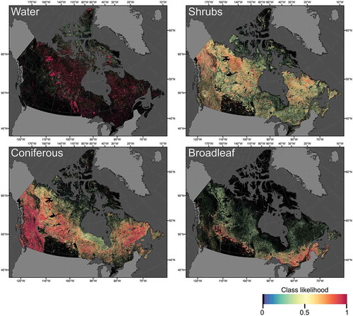
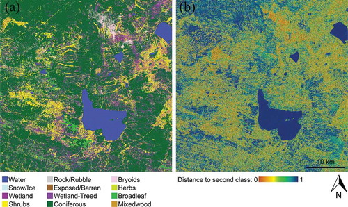
Additionally, these posteriori class probabilities enable relative confidence maps to be derived, enriching the land cover product suite. In this sense, layers such as distance to the second class based on the post-classification probabilities (Figure 3; Mitchell et al. 2008) or per-pixel predicted accuracy maps (Khatami, Mountrakis, and Stehman 2017) facilitate confidence building for the derived products, increasing the transparency of the mapping process and enabling regions of interest to be highlighted. Moreover, class probabilities provide the opportunity for end users with different information needs to combine or reassess classes allocated and/or probabilities assigned for a given year or over time (Comber, Law, and Lishman 2004). The uncertainty emerging from a mapping process can be used as information to alter categories or to alert map users or producers where issues may be present. A land cover map remains a single interpretation of reality (where many possible interpretations may exist), mediated by the information needs and application of the end user (Comber, Fisher, and Wadsworth 2005). Given current practices and algorithms, it is possible to carry and convey the uncertainty between classes rather than leaving pixels unclassified or classified without reference to confidence (e.g., Foody 1996; Mitchell et al. 2008). For additional examples for incorporating per-pixel information to improve map results or better understand uncertainties, see McIver and Friedl (2001) and Friedl et al. (2010).

Figure 3. Example land cover classification (a) with distance to second class heat map (b). The example is located near Kotcho Lake in northwest British Columbia, Canada (Lat/Long: 59.06816°N/121.14950°W). High confidence classes (e.g., water) have large distances to second class based on the post-classification probabilities. Large distances to second class are also noted for homogeneous extents of forest. Lower distances to second class, denoting less confidence in the allocated category, are found for more rare and spatially limited classes (e.g., bryoids) or classes that have spectral similarity (e.g., herb, shrub, and broadleaf).

4.4. Trends, opportunities, and directions in land cover

Given the contemporary context of Land Cover 2.0 in juxtaposition to the institutional and scientific limitations outlined by Townshend (1992) where will the science and application of land cover be 25 years from now? Remote sensing is a rapidly changing and highly dynamic field. There is an increasing number of satellites capturing data at scales relevant to human interactions with the landscape. The large missions that are the purview of national space agencies are no longer the only sources of data, with commercial data options proliferating. The niches currently filled by government and commercial satellite operators are diverging, with commercial vendors availing upon new, lower cost technologies and launch opportunities to place large numbers of small-satellites into orbit. What these small satellites lack in radiometric consistency, spectral bands, and orbital stability, is somewhat offset by their high spatial resolution and frequent temporal revisit period. Determination of how to integrate data across the range of space-based measures will provide additional monitoring and land cover mapping opportunities. In the future, land cover applications that are not reliant on a specific data stream will likely emerge (e.g., Yu, Wang, and Gong 2013; Chen et al. 2015), increasing the flexibility and speed with which land cover information can be generated (e.g., Zhang and Roy 2017).

A key facet of Land Cover 2.0 will be the use of data from different satellites to provide more complete spatial mosaics and/or richer time series for land cover classification purposes. Arguably, differences between different sensor data can be overcome if large amounts of training data are used, although, as discussed above, appropriate training data collection can be challenging. Alternatively, the different sensor data may be processed to be more compatible for classification purposes. To achieve this, the different sensor data may be combined to provide a sensor fusion product, or may be kept separate but harmonized so that the processed data may be used more reliably together. The former fusion approach strictly requires that the data from each sensor are precisely co-registered, calibrated, spectrally normalized to common wavebands, atmospherically corrected (using the same atmospheric characterization), and corrected for surface anisotropy. Sensor data fusion has been undertaken using physically based approaches, for example, by inverting Bidirectional Reflectance Distribution Function (BRDF) models using reflectance data from different sensors (Jin et al. 2002; Schaaf et al. 2002). Sensor data harmonization can be undertaken in a more empirical manner, for example, by computation of spectral vegetation indices derived from different sensors, and/or by applying statistical transformations between similar bands of different sensors (Brown et al. 2006; Miura, Huete, and Yoshioka 2006; Roy et al. 2016c; Zhang et al. In review). Ideally, these approaches will enable interchangeable and combined sensor data use as part of an integrated workflow (or elements of a virtual constellation, Wulder et al. 2015). However, this becomes challenging if the satellite data and resolution characteristics and quality differ significantly. For example, research on the use of MODIS and Landsat data for classification purposes is well established (Hansen et al. 2008). Integration of these data with newer commercial remote sensing systems, which may be of lower spectral quality but higher spatial and temporal resolution, offers unique opportunities but additional investigation is required (e.g., Houborg and McCabe 2018).

A greater integration of modeling with remote sensing could also be expected. Over terrestrial ecosystems, deterministic processes are at play. For example, disturbed forests return in a relatively consistent sequence of cover types, and agricultural cropping patterns are likewise not random. Models projecting a given land cover condition can be statistically confirmed or denied, thereby reducing reliance on satellite observations to provide a unique information outcome, and offering opportunities to increase product temporal density or spatial detail. Furthermore, data assimilation has been shown to offer new opportunities for integrating remotely sensed data and models beyond land cover, such as in the generation of other forest inventory information (Nyström et al. 2015). Integration of data from different sensors with disparate spectral and spatial resolutions may also be enabled through a combined modeling and remote sensing approach. This integrated approach could serve to reduce the need for radiometric uniformity across an envisioned data stream (opening opportunities for CubeSat, for instance). Caution must be exercised with regards to the radiometry and spectral consistency of CubeSat data (Houborg and McCabe 2018). Large numbers of CubeSat images are required to represent areas of the extents discussed herein (regional, continental, to global). Differences in view angles and illumination conditions can be expected, which serves to reduce spectral comparability, as well as the science and applications possible. Non-calibrated data sources may be useful for capturing change but will be limited for the more broad suite of attributes desired of remote sensing (land cover, biophysical estimates, or capture of subtle change or trends). Here, the distinction between the use of images as pictures versus the use of images as calibrated observations must be made; the two products service different information needs and have different utility in a long-term land cover monitoring context.

The capacity to generate land cover information in near-real time is a logical progression from the aforementioned prospects for integrating different data sources and modelling approaches into land cover product development. Many stakeholders would benefit from reduced latency and increased consistency in obtaining information on when, and where, land cover change is occurring (e.g., deforestation, illegal logging, wildfire, disaster response). While the need is evident with methods currently under development (Zhu and Woodcock 2014b), the nature, timing, and detail of what is reported in near-real time remains to be determined. Given the data storage and download capacity now possible, data can increasingly be collected in an ‘always-on’ mode. This would provide the regular, consistent within-year measures that are required for near-real time algorithms. Moreover, increasingly sophisticated automated ground systems reduce the latency in end-user data access. The fusion of data from a number of complementary sensors is also poised to become increasingly common to inform near real-time applications.

5. Conclusions

It is evident that much progress has been made in addressing both the data and methodological limitations identified by Townshend (1992). It can also be stressed that many of the institutional or programmatic barriers to the ‘provision of reliable operational land cover information from satellite data’ identified by Townshend (1992), have also been removed or have ceased to be the barriers they once were. Today, many national or regional programs rely on land cover information generated from Earth observation data to support monitoring efforts and inform science and policy (e.g., Bossard, Feranec, and Otahel 2000; Wickham et al. 2014). Ultimately, the greatest need for reliable land cover information has not changed since Townshend (1992): that of improving our understanding of drivers and processes of global change.

The work of Townshend (1992) provides an important benchmark in the evolution of remote sensing science. Advances towards reliable operational land cover products have been made on many fronts in the past 25 years. Land cover and land cover change are now a fully integrated information output. Today, land cover information can be operationally generated in an increasingly automated, systematic, and rigorous fashion. As a concept, Land Cover 2.0, brings together disparate advancements in data sources and policies, algorithms, and computational capacity. Open data has fueled the rapid development in land cover science and application, and set the stage for future innovations in land cover products and applications. An increasingly diverse set of data are at the core of the Land Cover 2.0 concept, with quality reference data remaining an important priority.

The manner in which reference data are acquired, standardized, and shared will be a critical to the quality of products generated through Land Cover 2.0. The use of reference data for independent validation of land cover products will be critical, with transparent and robust methods to be implemented, and a broader suite of confidence building layers of interest to modellers, data users, and policy makers. Building on the insights and experiences of the remote sensing community, land cover 2.0 provides an opportunity to meet the information needs of a number of stakeholders and to approach the vision of early scientists and practitioners. The rapidly developing technological (satellite, communications, computing) and applications landscape will continue to evolve and further empower science in support of pressing interests of society.

Acknowledgments

This research was undertaken as part of the “Earth observation to inform Canada’s climate change agenda (EO3C)” project jointly funded by the Canadian Space Agency (CSA), Government Related Initiatives (GRI), and the Canadian Forest Service (CFS) of Natural Resources Canada. Support was also provided by a Natural Sciences and Engineering Research Council of Canada (NSERC, RGPIN 311926-13) grant to Coops. Indication of commercial products or services does not indicate or imply endorsement. The Editor and Reviewers are thanked for valuable insights and guidance that improved the quality and content of this paper.

Disclosure statement

No potential conflict of interest was reported by the authors.

References

- GCOS. 2011. “Systematic Observation Requirements for Satellite-Based Products for Climate Supplemental Details to the Satellite-Based Component of the Implementation Plan for the Global Observing System for Climate in Support of the UNFCCC - (2011 Update).” In GCOS-154, edited by A. Simmons. Geneva, Switzerland: United Nations Environment Programme, World Meteorological Organization and International Council for Science. https://library.wmo.int/opac/doc_num.php?explnum_id=3710
- Abercrombie, S. P., and M. A. Friedl. 2016. “Improving the Consistency of Multitemporal Land Cover Maps Using a Hidden Markov Model.” IEEE Transactions on Geoscience and Remote Sensing 54 (2): 703–713. doi:10.1109/TGRS.2015.2463689.
- Anderson, J. R., E. Hardy, J. Roach, and R. Witmer. 1976. “A Land Use and Land Cover Classification System for Use with Remote Sensor Data.” USGS Professional Paper 964. p. 28. Washington, DC: United States Government Printing Office.
- Andrew, M. E., M. A. Wulder, and T. A. Nelson. 2014. “Potential Contributions of Remote Sensing to Ecosystem Service Assessments.” Progress in Physical Geography 38 (3): 328–353. doi:10.1177/0309133314528942.
- Azzari, G., and D. B. Lobell. 2017. “Landsat-Based Classification in the Cloud: An Opportunity for a Paradigm Shift in Land Cover Monitoring.” Remote Sensing of Environment 202: 64–74. doi:10.1016/j.rse.2017.05.025.
- Beaubien, J., J. Cihlar, G. Simard, and R. Latifovic. 1999. “Land Cover from Multiple Thematic Mapper Scenes Using a New Enhancement-Classification Methodology.” Journal of Geophysical Research: Atmospheres 104 (D22): 27909–27920. doi:10.1029/1999JD900243.
- Belgiu, M., and L. Drăguţ. 2016. “Random Forest in Remote Sensing: A Review of Applications and Future Directions.” ISPRS Journal of Photogrammetry and Remote Sensing 114: 24–31. doi:10.1016/j.isprsjprs.2016.01.011.
- Belward, A. S., and J. O. Skøien. 2015. “Who Launched What, When and Why; Trends in Global Land-Cover Observation Capacity from Civilian Earth Observation Satellites.” ISPRS Journal of Photogrammetry and Remote Sensing 103: 115–128. doi:10.1016/j.isprsjprs.2014.03.009.
- Boisvenue, C., B. P. Smiley, J. C. White, W. A. Kurz, and M. A. Wulder. 2016. “Improving Carbon Monitoring and Reporting in Forests Using Spatially-Explicit Information.” Carbon Balance and Management 11 (1): 23. doi:10.1186/s13021-016-0065-6.
- Boryan, C., Z. Yang, R. Mueller, and M. Craig. 2011. “Monitoring US Agriculture: The US Department of Agriculture, National Agricultural Statistics Service, Cropland Data Layer Pro-Gram.” Geocarto International 26: 341–358. doi:10.1080/10106049.2011.562309.
- Bossard, M., J. Feranec, and J. Otahel. 2000. CORINE Land Cover Technical Guide: Addendum 2000. Copenhagen, Denmark: European Environment Agency (EEA).
- Breiman, L. 2001. “Random Forests.” Machine Learning 45: 5–32. doi:10.1023/A:1010933404324.
- Breiman, L., J. H. Friedman, R. Olshen, and C. J. Stone. 1984. Classification and Regression Trees. Belmont: Wadworth.
- Brown, M. E., J. E. Pinzón, K. Didan, J. T. Morisette, and C. J. Tucker. 2006. “Evaluation of the Consistency of Long-Term NDVI Time Series Derived from AVHRR, SPOT-vegetation, SeaWiFS, MODIS, and Landsat ETM+ Sensors.” IEEE Transactions on Geoscience and Remote Sensing 44 (7): 1787–1793. doi:10.1109/TGRS.2005.860205.
- Cai, S., D. Liu, D. Sulla-Menashe, and M. A. Friedl. 2014. “Enhancing MODIS Land Cover Product with a Spatial–Temporal Modeling Algorithm.” Remote Sensing of Environment 147: 243–255. doi:10.1016/j.rse.2014.03.012.
- CEOS. 2017. “Committee on Earth Observation Satellites Data Cube.” Open Data Cube. Accessed February 2018. https://www.opendatacube.org/ceos
- Champagne, C., H. McNairn, B. Daneshfar, and J. Shang. 2014. “A Bootstrap Method for Assessing Classification Accuracy and Confidence for Agricultural Land Use Mapping in Canada.” International Journal of Applied Earth Observation and Geoinformation 29: 44–52. doi:10.1016/j.jag.2013.12.016.
- Chavez, P. S. 1988. “An Improved Dark-Object Subtraction Technique for Atmospheric Scattering Correction of Multispectral Data.” Remote Sensing of Environment 24 (3): 459–479. doi:10.1016/0034-4257(88)90019-3.
- Chen, J., J. Chen, A. Liao, X. Cao, L. Chen, X. Chen, C. He, et al. 2015. “Global Land Cover Mapping at 30m Resolution: A POK-based Operational Approach.” ISPRS Journal of Photogrammetry and Remote Sensing 103: 7–27. doi:10.1016/j.isprsjprs.2014.09.002.
- Chen, Z., N. Chen, C. Yang, and L. Di. 2012. “Cloud Computing Enabled Web Processing Service for Earth Observation Data Processing.” IEEE Journal of Selected Topics in Applied Earth Observations and Remote Sensing 5 (6): 1637–1649. doi:10.1109/JSTARS.2012.2205372.
- Cihlar, J. 2000. “Land Cover Mapping of Large Areas from Satellites: Status and Research Priorities.” International Journal of Remote Sensing 21 (6 & 7): 1093–1114. doi:10.1080/014311600210092.
- Collins, J. B., and C. E. Woodcock. 1996. “An Assessment of Several Linear Change Detection Techniques for Mapping Forest Mortality Using Multitemporal Landsat TM Data.” Remote Sensing of Environment 56 (1): 66–77. doi:10.1016/0034-4257(95)00233-2.
- Comber, A., C. Fonte, G. Foody, S. Fritz, P. Harris, A.-M. Olteanu-Raimond, and L. See. 2016. “Geographically-Weighted Evidence Combination Approaches for Combining Discordant and Inconsistent Volunteered Geographical Information.” GeoInformatica 20 (3): 503–527. doi:10.1007/s10707-016-0248-z.
- Comber, A., P. Fisher, and R. Wadsworth. 2005. “What Is Land Cover?” Environment and Planning B: Planning and Design 32 (2): 199–209. doi:10.1068/b31135.
- Comber, A. J., A. N. R. Law, and J. R. Lishman. 2004. “Application of Knowledge for Automated Land Cover Change Monitoring.” International Journal of Remote Sensing 25 (16): 3177–3192. doi:10.1080/01431160310001657795.
- Courtois, M., and M. Traizet. 1986. “The SPOT Satellites: From SPOT 1 to SPOT 4.” Geocarto International 1 (3): 4–14. doi:10.1080/10106048609354050.
- de Colstoun, E. C. B., and C. L. Walthall. 2006. “Improving Global Scale Land Cover Classifications with Multi-Directional POLDER Data and a Decision Tree Classifier.” Remote Sensing of Environment 100 (4): 474–485. doi:10.1016/j.rse.2005.11.003.
- DeFries, R., M. Hansen, and J. Townshend. 1995. “Global Discrimination of Land Cover Types from Metrics Derived from AVHRR Pathfinder Data.” Remote Sensing of Environment 54: 209–222. doi:10.1016/0034-4257(95)00142-5.
- DeFries, R. S., J. A. Foley, and G. P. Asner. 2004. “Land-Use Choices: Balancing Human Needs and Ecosystem Function.” Frontiers in Ecology and the Environment 2 (5): 249–257. doi:10.1890/1540-9295(2004)002[0249:LCBHNA]2.0.CO;2.
- DeFries, R. S., R. A. Houghton, M. C. Hansen, C. B. Field, D. Skole, and J. Townshend. 2002. “Carbon Emissions from Tropical Deforestation and Regrowth Based on Satellite Observations for the 1980s and 1990s.” Proceedings of the National Academy of Sciences of the United States of America 99 (22): 14256–14261. doi:10.1073/pnas.182560099.
- Di Gregorio, A. 2005. Land Cover Classification System: Classification Concepts and User Manual: LCCS (No. 8). Rome, Italy: Food and Agriculture Organization.
- Doan, H. T. X., and G. M. Foody. 2007. “Increasing Soft Classification Accuracy through the Use of an Ensemble of Classifiers.” International Journal of Remote Sensing 28: 4609–4623. doi:10.1080/01431160701244872.
- Dobson, M. C., F. T. Ulaby, and L. E. Pierce. 1995. “Land-Cover Classification and Estimation of Terrain Attributes Using Synthetic Aperture Radar.” Remote Sensing of Environment 51: 199–214. doi:10.1016/0034-4257(94)00075-X.
- Drusch, M., U. Del Bello, S. Carlier, O. Colin, V. Fernandez, F. Gascon, B. Hoersch, C. Isola, P. Laberinti, and P. Martimort. 2012. “Sentinel-2: ESA’s Optical High-Resolution Mission for GMES Operational Services.” Remote Sensing of Environment 120: 25–36. doi:10.1016/j.rse.2011.11.026.
- Egorov, A. V., M. C. Hansen, D. P. Roy, A. Kommareddy, and P. V. Potapov. 2015. “Image Interpretation-Guided Supervised Classification Using Nested Segmentation.” Remote Sensing of Environment 165: 135–147. doi:10.1016/j.rse.2015.04.022.
- Eidenshink, J. C., and J. L. Faudeen. 1994. “The 1 Km AVHRR Global Land Data Set: First Stages in Implementation.” International Journal of Remote Sensing 15: 3443–3462. doi:10.1080/01431169408954339.
- Foga, S., P. L. Scaramuzza, S. Guo, Z. Zhu, R. D. Dilley, T. Beckmann, G. L. Schmidt, J. L. Dwyer, M. J. Hughes, and B. Laue. 2017. “Cloud Detection Algorithm Comparison and Validation for Operational Landsat Data Products.” Remote Sensing of Environment 194: 379–390. doi:10.1016/j.rse.2017.03.026.
- Foody, G. M. 1996. “Approaches for the Production and Evaluation of Fuzzy Land Cover Classifications from Remotely-Sensed Data.” International Journal of Remote Sensing 17 (7): 1317–1340. doi:10.1080/01431169608948706.
- Foody, G. M. 2002. “Status of Land Cover Classification Accuracy Assessment.” Remote Sensing of Environment 80 (1): 185–201. doi:10.1016/S0034-4257(01)00295-4.
- Foody, G. M., L. See, S. Fritz, M. Van der Velde, C. Perger, C. Schill, D. S. Boyd, and A. Comber. 2015. “Accurate Attribute Mapping from Volunteered Geographic Information: Issues of Volunteer Quantity and Quality.” The Cartographic Journal 52 (4): 336–344. doi:10.1179/1743277413Y.0000000070.
- Franklin, S. E., and M. A. Wulder. 2002. “Remote Sensing Methods in Medium Spatial Resolution Satellite Data Land Cover Classification of Large Areas.” Progress in Physical Geography 26 (2): 173–205. doi:10.1191/0309133302pp332ra.
- Frantz, D., A. Röder, M. Stellmes, and J. Hill. 2017. “Phenology-Adaptive Pixel-Based Compositing Using Optical Earth Observation Imagery.” Remote Sensing of Environment 190: 331–347. doi:10.1016/j.rse.2017.01.002.
- Frey, R. A., S. A. Ackerman, Y. Liu, K. I. Strabala, H. Zhang, J. R. Key, and X. Wang. 2008. “Cloud Detection with MODIS. Part I: Improvements in the MODIS Cloud Mask for Collection 5.” Journal of Atmospheric and Oceanic Technology 25 (7): 1057–1072. doi:10.1175/2008JTECHA1052.1.
- Friedl, M. A., D. Sulla-Menashe, B. Tan, A. Schneider, N. Ramankutty, A. Sibley, and X. Huang. 2010. “MODIS Collection 5 Global Land Cover: Algorithm Refinements and Characterization of New Datasets.” Remote Sensing of Environment 114 (1): 168–182. doi:10.1016/j.rse.2009.08.016.
- Friedl, M. A., D. K. McIver, J. C. Hodges, X. Y. Zhang, D. Muchoney, A. H. Strahler, C. E. Woodcock, et al. 2002. “Global Land Cover Mapping from MODIS: Algorithms and Early Results.” Remote Sensing of Environment 83 (1): 287–302. doi:10.1016/S0034-4257(02)00078-0.
- Fritz, S., I. McCallum, C. Schill, C. Perger, L. See, D. Schepaschenko, M. Van der Velde, F. Kraxner, and M. Obersteiner. 2012. “Geo-Wiki: An Online Platform for Improving Global Land Cover.” Environmental Modelling and Software 31: 110–123. doi:10.1016/j.envsoft.2011.11.015.
- Fritz, S., L. See, C. Perger, I. McCallum, C. Schill, D. Schepaschenko, M. Duerauer, et al. 2017. “A Global Dataset of Crowdsourced Land Cover and Land Use Reference Data.” Scientific Data 4: 170075. doi:10.1038/sdata.2017.75.
- Fuller, R. M., G. B. Groom, and A. R. Jones. 1994. “The Landcover Map of Great Britain: An Automated Classification of Landsat Thematic Mapper Data.” Photogrammetric Engineering and Remote Sensing 60: 553–562.
- Fuller, R. M., G. M. Smith, and B. J. Devereux. 2003. “The Characterisation and Measurement of Land Cover Change through Remote Sensing: Problems in Operational Applications?” International Journal of Applied Earth Observation and Geoinformation 4 (3): 243–253. doi:10.1016/S0303-2434(03)00004-7.
- Gao, F., J. Masek, M. Schwaller, and F. Hall. 2006. “On the Blending of the Landsat and MODIS Surface Reflectance: Predicting Daily Landsat Surface Reflectance.” IEEE Transactions on Geoscience and Remote Sensing 44 (8): 2207–2218. doi:10.1109/TGRS.2006.872081.
- Gascon, F., C. Bouzinac, O. Thépaut, M. Jung, B. Francesconi, J. Louis, V. Lonjou, et al. 2017. “Copernicus Sentinel-2A Calibration and Products Validation Status.” Remote Sensing 9 (6): 584. doi:10.3390/rs9060584.
- GCOS. 2016. “The Global Observing System for Climate: Implementation Needs.” GCOS 200 (GOOS-214), 325. Geneva: World Meteorological Organisation. Accessed October 25 2017. https://unfccc.int/files/science/workstreams/systematic_observation/application/pdf/gcos_ip_10oct2016.pdf
- Gislason, P. O., J. A. Benediktsson, and J. R. Sveinsson. 2006. “Random Forests for Land Cover Classification.” Pattern Recognition Letters 27 (4): 294–300. doi:10.1016/j.patrec.2005.08.011.
- Gómez, C., J. C. White, and M. A. Wulder. 2016. “Optical Remotely Sensed Time Series Data for Land Cover Classification: A Review.” ISPRS Journal of Photogrammetry and Remote Sensing 116: 55–72. doi:10.1016/j.isprsjprs.2016.03.008.
- Gong, P., J. Wang, L. Yu, Y. Zhao, Y. Zhao, L. Liang, Z. Niu, et al. 2013. “Finer Resolution Observation and Monitoring of Global Land Cover: First Mapping Results with Landsat TM and ETM+ Data.” International Journal of Remote Sensing 34 (7): 2607–2654. doi:10.1080/01431161.2012.748992.
- Gong, W., S. Fang, G. Yang, and M. Ge. 2017. “Using a Hidden Markov Model for Improving the Spatial-Temporal Consistency of Time Series Land Cover Classification.” ISPRS International Journal of Geo-Information 6 (10): 292.
- Gorelick, N., M. Hancher, M. Dixon, S. Ilyushchenko, D. Thau, and R. Moore. 2017. “Google Earth Engine: Planetary-Scale Geospatial Analysis for Everyone.” Remote Sensing of Environment 202: 18–27. doi:10.1016/j.rse.2017.06.031.
- Gray, J., and C. Song. 2013. “Consistent Classification of Image Time Series with Automatic Adaptive Signature Generalization.” Remote Sensing of Environment 134: 333–341. doi:10.1016/j.rse.2013.03.022.
- Grekousis, G., G. Mountrakis, and M. Kavouras. 2015. “An Overview of 21 Global and 43 Regional Land-Cover Mapping Products.” International Journal of Remote Sensing 36: 5309–5335. doi:10.1080/01431161.2015.1093195.
- Griffiths, P., S. van der Linden, T. Kuemmerle, and P. Hostert. 2013. “A Pixel-Based Landsat Compositing Algorithm for Large Area Land Cover Mapping.” IEEE Journal of Selected Topics in Applied Earth Observations and Remote Sensing 6 (5): 2088–2101. doi:10.1109/JSTARS.2012.2228167.
- Gutiérrez-Vélez, V. H., and R. DeFries. 2013. “Annual Multi-Resolution Detection of Land Cover Conversion to Oil Palm in the Peruvian Amazon.” Remote Sensing of Environment 129: 154–167. doi:10.1016/j.rse.2012.10.033.
- GWELD. 2017. “Global WELD Data, Collections.” Version 3. Accessed February 2018. https://gweld-download.cr.usgs.gov/collections/
- Hansen, M. C., A. Egorov, D. P. Roy, P. Potapov, J. Ju, S. Turubanova, I. Kommareddy, and T. R. Loveland. 2011. “Continuous Fields of Land Cover for the Conterminous United States Using Landsat Data: First Results from the Web-Enabled Landsat Data (WELD) Project.” Remote Sensing Letters 2: 279–288. doi:10.1080/01431161.2010.519002.
- Hansen, M. C., D. P. Roy, E. Lindquist, B. Adusei, C. O. Justice, and A. Altstaat. 2008. “A Method for Integrating MODIS and Landsat Data for Systematic Monitoring of Forest Cover and Change and Preliminary Results for Central Africa.” Remote Sensing of Environment 112: 2495–2513. doi:10.1016/j.rse.2007.11.012.
- Hansen, M. C., P. V. Potapov, R. Moore, M. Hancher, S. A. Turubanova, A. Tyukavina, D. Thau, et al. 2013. “High-Resolution Global Maps of 21st-Century Forest Cover Change.” Science 342 (6160): 850–853. doi:10.1126/science.1244693.
- Hansen, M. C., R. S. DeFries, J. R. Townshend, and R. Sohlberg. 2000. “Global Land Cover Classification at 1 Km Spatial Resolution Using a Classification Tree Approach.” International Journal of Remote Sensing 21 (6–7): 1331–1364. doi:10.1080/014311600210209.
- Henderson, R. G. 1976. “Signature Extension Using the MASC Algorithm.” IEEE Transactions on Geoscience Electronics 14 (1): 34–37. doi:10.1109/TGE.1976.294462.
- Hermosilla, T., M. A. Wulder, J. C. White, N. C. Coops, and G. W. Hobart. 2015a. “An Integrated Landsat Time Series Protocol for Change Detection and Generation of Annual Gap-Free Surface Reflectance Composites.” Remote Sensing of Environment 158: 220–234. doi:10.1016/j.rse.2014.11.005.
- Hermosilla, T., M. A. Wulder, J. C. White, N. C. Coops, and G. W. Hobart. 2015b. “Regional Detection, Characterization, and Attribution of Annual Forest Change from 1984 to 2012 Using Landsat-Derived Time-Series Metrics.” Remote Sensing of Environment 170: 121–132. doi:10.1016/j.rse.2015.09.004.
- Hermosilla, T., M. A. Wulder, J. C. White, N. C. Coops, and G. W. Hobart. 2018. “Disturbance-Informed Annual Land Cover Classification with Landsat Time Series: A 29-Year National Data Cube.” Canadian Journal of Remote Sensing. doi:10.1080/07038992.2018.1437719.
- Hermosilla, T., M. A. Wulder, J. C. White, N. C. Coops, G. W. Hobart, and L. B. Campbell. 2016. “Mass Data Processing of Time Series Landsat Imagery: Pixels to Data Products for Forest Monitoring.” International Journal of Digital Earth 9 (11): 1035–1054. doi:10.1080/17538947.2016.1187673.
- Herold, M., P. Mayaux, C. E. Woodcock, A. Baccini, and C. Schmullius. 2008. “Some Challenges in Global Land Cover Mapping: An Assessment of Agreement and Accuracy in Existing 1 Km Datasets.” Remote Sensing of Environment 112 (5): 2538–2556. doi:10.1016/j.rse.2007.11.013.
- Hilker, T., M. A. Wulder, N. C. Coops, J. Linke, G. McDermid, J. G. Masek, F. Gao, and J. C. White. 2009. “A New Data Fusion Model for High Spatial-And Temporal-Resolution Mapping of Forest Disturbance Based on Landsat and MODIS.” Remote Sensing of Environment 113 (8): 1613–1627. doi:10.1016/j.rse.2009.03.007.
- Holben, B. 1986. “Characteristics of Maximum-Value Composite Images from Temporal AVHRR Data.” International Journal of Remote Sensing 7: 1417–1434. doi:10.1080/01431168608948945.
- Houborg, R., and M. F. McCabe. 2018. “A Cubesat Enabled Spatio-Temporal Enhancement Method (CESTEM) Utilizing Planet, Landsat and MODIS Data.” Remote Sensing of Environment.
- Inglada, J., A. Vincent, M. Arias, B. Tardy, D. Morin, and I. Rodes. 2017. “Operational High Resolution Land Cover Map Production at the Country Scale Using Satellite Image Time Series.” Remote Sensing 9 (12): 95. doi:10.3390/rs9010095.
- Janssen, L. L. F., and F. J. M. van der Wel. 1994. “Accuracy Assessment of Satellite Derived Land-Cover Data: A Review.” Photogrammetric Engineering and Remote Sensing 60 (4): 419–426.
- Jayaraman, P. P., C. Perera, D. Georgakopoulos, S. Dustdar, D. Thakker, and R. Ranjan. 2017. “Analytics‐As‐A‐Service in a Multi‐Cloud Environment through Semantically‐Enabled Hierarchical Data Processing.” Software: Practice and Experience 47 (8): 1139–1156.
- Jin, Y., F. Gao, C. B. Schaaf, X. Li, A. H. Strahler, C. J. Bruegge, and J. V. Martonchik. 2002. “Improving MODIS Surface BRDF/albedo Retrieval with MISR Multiangle Observations.” IEEE Transactions on Geoscience and Remote Sensing 40 (7): 1593–1604. doi:10.1109/TGRS.2002.801145.
- Johnson, D. M., and R. Mueller. 2010. “The 2009 Cropland Data Layer.” Photogrammetric. Engineering and Remote Sensing. 76: 1201–1205.
- Journaux, L., I. Foucherot, and P. Gouton. 2006. “Reduction of the Number of Spectral Bands in Landsat Images: A Comparison of Linear and Nonlinear Methods.” Optical Engineering 45 (6): 067002–067003. doi:10.1117/1.2212108.
- Ju, J., D. P. Roy, E. Vermote, J. Masek, and V. Kovalskyy. 2012. “Continental-Scale Validation of MODIS-based and LEDAPS Landsat ETM+ Atmospheric Correction Methods.” Remote Sensing of Environment 122: 175–184. doi:10.1016/j.rse.2011.12.025.
- Jung, M., K. Henkel, M. Herold, and G. Churkina. 2006. “Exploiting Synergies of Global Land Cover Products for Carbon Cycle Modeling.” Remote Sensing of Environment 101 (4): 534–553. doi:10.1016/j.rse.2006.01.020.
- Justice, C., E. Vermote, J. Townshend, R. Defries, D. Roy, D. Hall, V. Salomonson, et al. 1998. “The Moderate Resolution Imaging Spectroradiometer (MODIS): Land Remote Sensing for Global Change Research.” IEEE Transactions on Geoscience and Remote Sensing 36: 1228–1249. doi:10.1109/36.701075.
- Justice, C., J. Townshend, E. Vermote, E. Masuoka, R. Wolfe, N. Saleous, D. Roy, and J. Morisette. 2002. “An Overview of MODIS Land Data Processing and Product Status.” Remote Sensing of Environment 83: 3–15. doi:10.1016/S0034-4257(02)00084-6.
- Khatami, R., G. Mountrakis, and S. V. Stehman. 2016. “A Meta-Analysis of Remote Sensing Research on Supervised Pixel-Based Land-Cover Image Classification Processes: General Guidelines for Practitioners and Future Research.” Remote Sensing of Environment 177: 89–100. doi:10.1016/j.rse.2016.02.028.
- Khatami, R., G. Mountrakis, and S. V. Stehman. 2017. “Mapping Per-Pixel Predicted Accuracy of Classified Remote Sensing Images.” Remote Sensing of Environment 191: 156–167. doi:10.1016/j.rse.2017.01.025.
- Kovalskyy, V., and D. P. Roy. 2013. “The Global Availability of Landsat 5 TM and Landsat 7 ETM+ Land Surface Observations and Implications for Global 30 M Landsat Product Generation.” Remote Sensing of Environment 130: 280–293. doi:10.1016/j.rse.2012.12.003.
- Lewis, A., S. Oliver, L. Lymburner, B. Evans, L. Wyborn, N. Mueller, G. Raevksi, et al. 2017. “The Australian Geoscience Data Cube - Foundations and Lessons Learned.” Remote Sensing of Environment. doi:10.1016/j.rse.2017.03.015.
- Li, J., and D. P. Roy. 2017. “A Global Analysis of Sentinel-2A, Sentinel-2B and Landsat-8 Data Revisit Intervals and Implications for Terrestrial Monitoring.” Remote Sensing 9 (9): 902. doi:10.3390/rs9090902.
- Li, W., P. Ciais, S. Peng, Y. Chao, Y. Wang, M. Thurner, S. S. Saatchi, et al. 2017a. “Land-Use and Land-Cover Change Carbon Emissions between 1901 and 2012 Constrained by Biomass Observations.” Biogeosciences 14 (22): 5053. doi:10.5194/bg-14-5053-2017.
- Li, Z., H. K. Zhang, D. P. Roy, L. Yan, H. Huang, J. Li, and Z. Li. 2017b. “Landsat 15 M Panchromatic Assisted Downscaling (LPAD) of 30 M Reflective Wavelength Data to Sentinel-2 20 M Resolution.” Remote Sensing 9 (7): 755. doi:10.3390/rs9070755.
- Lindquist, E., M. C. Hansen, D. P. Roy, and C. O. Justice. 2008. “The Suitability of Decadal Image Data Sets for Mapping Tropical Forest Cover Change in the Democratic Republic of Congo: Implications for the Mid-Decadal Global Land Survey.” International Journal of Remote Sensing 29: 7269–7275. doi:10.1080/01431160802275890.
- Liu, H., and Q. Zhou. 2004. “Accuracy Analysis of Remote Sensing Change Detection by Rule-Based Rationality Evaluation with Post-Classification Comparison.” International Journal of Remote Sensing 25 (5): 1037–1050. doi:10.1080/0143116031000150004.
- Loveland, T. R., B. C. Reed, J. F. Brown, D. O. Ohlen, Z. Zhu, L. W. M. J. Yang, and J. W. Merchant. 2000. “Development of a Global Land Cover Characteristics Database and IGBP DISCover from 1 Km AVHRR Data.” International Journal of Remote Sensing 21 (6–7): 1303–1330. doi:10.1080/014311600210191.
- Mannan, B., J. Roy, and A. K. Ray. 1998. “Fuzzy ARTMAP Supervised Classification of Multi-Spectral Remotely-Sensed Images.” International Journal of Remote Sensing 19 (4): 767–774. doi:10.1080/014311698215991.
- McIver, D. K., and M. A. Friedl. 2001. “Estimating Pixel-Scale Land Cover Classification Confidence Using Nonparametric Machine Learning Methods.” IEEE Transactions on Geoscience and Remote Sensing 39 (9): 1959–1968. doi:10.1109/36.951086.
- Mellor, A., S. Boukir, A. Haywood, and S. Jones. 2015. “Exploring Issues of Training Data Imbalance and Mislabelling on Random Forest Performance for Large Area Land Cover Classification Using the Ensemble Margin.” ISPRS Journal of Photogrammetry and Remote Sensing 105: 155–168. doi:10.1016/j.isprsjprs.2015.03.014.
- Midekisa, A., F. Holl, D. J. Savory, R. Andrade-Pacheco, P. W. Gething, A. Bennett, and H. J. Sturrock. 2017. “Mapping Land Cover Change over Continental Africa Using Landsat and Google Earth Engine Cloud Computing.” PloS One 12 (9): e0184926. doi:10.1371/journal.pone.0184926.
- Millard, K., and M. Richardson. 2015. “On the Importance of Training Data Sample Selection in Random Forest Image Classification: A Case Study in Peatland Ecosystem Mapping.” Remote Sensing 7 (7): 8489–8515. doi:10.3390/rs70708489.
- Mitchell, S. W., T. K. Remmel, F. Csillag, and M. A. Wulder. 2008. “Distance to Second Cluster as a Measure of Classification Confidence.” Remote Sensing of Environment 112: 2615–2626. doi:10.1016/j.rse.2007.12.006.
- Miura, T., A. Huete, and H. Yoshioka. 2006. “An Empirical Investigation of Cross-Sensor Relationships of NDVI and Red/Near-Infrared Reflectance Using EO-1 Hyperion Data.” Remote Sensing of Environment 100 (2): 223–236. doi:10.1016/j.rse.2005.10.010.
- Morisette, J. T., J. E. Nickeson, P. Davis, Y. Wang, Y. Tian, C. E. Woodcock, N. Shabanov, et al. 2003. “High Spatial Resolution Satellite Observations for Validation of MODIS Land Products: IKONOS Observations Acquired under the NASA Scientific Data Purchase.” Remote Sensing of Environment 88 (1): 100–110. doi:10.1016/j.rse.2003.04.003.
- Müller, H., P. Rufin, P. Griffiths, L. D. B. V. Hissa, and P. Hostert. 2016. “Beyond Deforestation: Differences in Long-Term Regrowth Dynamics across Land Use Regimes in Southern Amazonia.” Remote Sensing of Environment 186: 652–662. doi:10.1016/j.rse.2016.09.012.
- Nemani, R., P. Votava, A. Michaelis, F. Melton, and C. Milesi. 2011. “Collaborative Supercomputing for Global Change Science.” Eos, Transactions American Geophysical Union. 92 (13): 109–110. doi:10.1029/2011EO130001.
- Nusser, S. M., and E. E. Klaas. 2003. “Survey Methods for Assessing Land Cover Map Accuracy.” Environmental and Ecological Statistics 10: 309–331. doi:10.1023/A:1025107023980.
- Nyström, M., N. Lindgren, J. Wallerman, A. Grafström, A. Muszta, K. Nyström, J. Bohlin, et al. 2015. “Data Assimilation in Forest Inventory: First Empirical Results.” Forests 6 (12): 4540–4557.
- Olofsson, P., G. M. Foody, M. Herold, S. V. Stehman, C. E. Woodcock, and M. A. Wulder. 2014. “Good Practices for Estimating Area and Assessing Accuracy of Land Change.” Remote Sensing of Environment 148: 42–57. doi:10.1016/j.rse.2014.02.015.
- Olofsson, P., S. V. Stehman, C. E. Woodcock, D. Sulla-Menashe, A. M. Sibley, J. D. Newell, M. A. Friedl, and M. Herold. 2012. “A Global Land-Cover Validation Data Set, Part I: Fundamental Design Principles.” International Journal of Remote Sensing 33 (18): 5768–5788.
- Pacifici, F., F. Del Frate, C. Solimini, and W. J. Emery. 2008. “Neural Networks for Land Cover Applications.” In Computational Intelligence for Remote Sensing. Studies in Computational Intelligence, edited by M. Graña and R. J. Duro. 133 vols. Berlin, Heidelberg: Springer.
- Pal, M., and P. M. Mather. 2005. “Support Vector Machines for Classification in Remote Sensing.” International Journal of Remote Sensing 26 (5): 1007–1011.
- Patenaude, G., R. Milne, and T. Dawson. 2005. “Synthesis of Remote Sensing Approaches for Forest Carbon Estimation: Reporting to the Kyoto Protocol.” Environmental Science & Policy 8: 161–178.
- Pelletier, C., S. Valero, J. Inglada, N. Champion, C. M. Sicre, and G. Dedieu. 2017. “Effect of Training Class Label Noise on Classification Performances for Land Cover Mapping with Satellite Image Time Series.” Remote Sensing 9 (2). doi:10.3390/rs9020173.
- Pelletier, C., S. Valero, J. Inglada, N. Champion, and G. Dedieu. 2016. “Assessing the Robustness of Random Forests to Map Land Cover with High Resolution Satellite Image Time Series over Large Areas.” Remote Sensing of Environment 187: 156–168.
- Pengra, B., J. Long, D. Dahal, S. V. Stehman, and T. R. Loveland. 2015. “A Global Reference Database from Very High Resolution Commercial Satellite Data and Methodology for Application to Landsat Derived 30m Continuous Field Tree Cover Data.” Remote Sensing of Environment 165: 234–248.
- Pettorelli, N., M. Wegmann, A. Skidmore, S. Mücher, T. P. Dawson, M. Fernandez, R. Lucas, et al. 2016. “Framing the Concept of Satellite Remote Sensing Essential Biodiversity Variables: Challenges and Future Directions.” Remote Sensing in Ecology and Conservation 2 (3): 122–131.
- Rodriguez-Galiano, V. F., B. Ghimire, J. Rogan, M. Chica-Olmo, and J. P. Rigol-Sanchez. 2012. “An Assessment of the Effectiveness of a Random Forest Classifier for Land-Cover Classification.” ISPRS Journal of Photogrammetry and Remote Sensing 67: 93–104.
- Rogan, J., and D. Chen. 2004. “Remote Sensing Technology for Mapping and Monitoring Land-Cover and Land-Use Change.” Progress in Planning 61 (4): 301–325.
- Rogan, J., J. Miller, D. Stow, J. Franklin, L. Levien, and C. Fischer. 2003. “Land-Cover Change Monitoring with Classification Trees Using Landsat TM and Ancillary Data.” Photogrammetric Engineering and Remote Sensing 69 (7): 793–804.
- Rosenqvist, A., A. Milne, R. Lucas, M. Imhoff, and C. Dobson. 2003. “A Review of Remote Sensing Technology in Support of the Kyoto Protocol.” Environmental Science and Policy 6: 441–455.
- Roy, D. P. 1997. “Investigation of the Maximum Normalised Difference Vegetation Index (NDVI) and the Maximum Surface Temperature (Ts) AVHRR Compositing Procedures for the Extraction of NDVI and Ts over Forest.” International Journal of Remote Sensing 18: 2383–2401.
- Roy, D. P., H. K. Zhang, J. Ju, J. L. Gomez-Dans, P. E. Lewis, C. B. Schaaf, Q. Sun, J. Li, H. Huang, and V. Kovalskyy. 2016b. “A General Method to Normalize Landsat Reflectance Data to Nadir BRDF Adjusted Reflectance.” Remote Sensing of Environment 176: 255–271.
- Roy, D. P., J. Ju, C. Mbow, P. Frost, and T. R. Loveland. 2010a. “Accessing Free Landsat Data via the Internet: Africa’s Challenge.” Remote Sensing Letters 1: 111–117.
- Roy, D. P., J. Ju, K. Kline, P. L. Scaramuzza, V. Kovalskyy, M. Hansen, T. R. Loveland, E. Vermote, and C. Zhang. 2010b. “Web-Enabled Landsat Data (WELD): Landsat ETM+ Composited Mosaics of the Conterminous United States.” Remote Sensing of Environment 114 (1): 35–49.
- Roy, D. P., J. Li, H. K. Zhang, and L. Yan. 2016a. “Best Practices for the Reprojection and Resampling of Sentinel-2 Multi Spectral Instrument Level 1C Data.” Remote Sensing Letters 7 (11): 1023–1032.
- Roy, D. P., M. A. Wulder, T. R. Loveland, C. E. Woodcock, R. G. Allen, M. C. Anderson, D. Helder, et al. 2014. “Landsat-8: Science and Product Vision for Terrestrial Global Change Research.” Remote Sensing of Environment 145: 154–172.
- Roy, D. P., V. Kovalskyy, H. K. Zhang, E. F. Vermote, L. Yan, S. S. Kumar, and A. Egorov. 2016c. “Characterization of Landsat-7 to Landsat-8 Reflective Wavelength and Normalized Difference Vegetation Index Continuity.” Remote Sensing of Environment 185: 57–70.
- Roy, D. P., Z. Li, and H. K. Zhang. 2017. “Adjustment of Sentinel-2 Multi-spectral Instrument (MSI) Red-edge Band Reflectance to Nadir BRDF Adjusted Reflectance (NBAR) and Quantification of Red-edge Band BRDF Effects.” Remote Sensing 9 (12): 1325.
- Running, S. W., T. R. Loveland, L. L. Pierce, R. R. Nemani, and E. R. Hunt. 1995. “A Remote Sensing Based Vegetation Classification Logic for Global Land Cover Analysis.” Remote Sensing of Environment 51 (1): 39–48.
- Schaaf, C. B., F. Gao, A. H. Strahler, W. Lucht, X. Li, T. Tsang, N. C. Strugnell, et al. 2002. “First Operational BRDF, Albedo Nadir Reflectance Products from MODIS.” Remote Sensing of Environment 83 (1–2): 135–148.
- Schott, J. R., C. Salvaggio, and W. K. Volchock. 1988. “Radiometric Scene Normalization Using Pseudo-Invariant Features.” Remote Sensing of Environment 26: 1−16.
- Schroeder, T. A., W. B. Cohen, C. Song, M. J. Canty, and Z. Yang. 2006. “Radiometric Correction of Multi-Temporal Landsat Data for Characterization of Early Successional Forest Patterns in Western Oregon.” Remote Sensing of Environment 103: 16–26.
- Scott, G. J., M. R. England, M. W. A. Starms, R. A. Marcum, and C. H. Davis. 2017. “Training Deep Convolutional Neural Networks for Land–cover Classification of High-resolution Imagery.” Ieee Geoscience and Remote Sensing Letters 14 (4): 549-553. doi:10.1109/LGRS.2017.2657778.
- Senf, C., P. J. Leitão, D. Pflugmacher, S. van der Linden, and P. Hostert. 2015. “Mapping Land Cover in Complex Mediterranean Landscapes Using Landsat: Improved Classification Accuracies from Integrating Multi-Seasonal and Synthetic Imagery.” Remote Sensing of Environment 156: 527–536.
- Skole, D., and C. Tucker. 1993. “Tropical Deforestation and Habitat Fragmentation in the Amazon: Satellite Data from 1978 to 1988.” Science 260 (5116): 1905–1910.
- Small, C., and D. Sousa. 2016. “Humans on Earth: Global Extents of Anthropogenic Land Cover from Remote Sensing.” Anthropocene 14: 1–33.
- Song, C., C. E. Woodcock, K. C. Seto, M. P. Lenney, and S. A. Macomber. 2001. “Classification and Change Detection Using Landsat TM Data: When and How to Correct Atmospheric Effects?” Remote Sensing of Environment 75 (2): 230–244.
- Stehman, S. V. 2009. “Sampling Designs for Accuracy Assessment of Land Cover.” International Journal of Remote Sensing 30 (20): 5243–5272.
- Stehman, S. V. 2013. “Estimating Area from an Accuracy Assessment Error Matrix.” Remote Sensing of Environment 132: 202–211.
- Stehman, S. V., P. Olofsson, C. E. Woodcock, M. Herold, and M. A. Friedl. 2012. “A Global Land-Cover Validation Data Set, II: Augmenting A Stratified Sampling Design to Estimate Accuracy by Region and Land-Cover Class.” International Journal of Remote Sensing 33 (22): 6975–6993.
- Strahler, A., T. Logan, and N. Bryant. 1978. “Improving Forest Cover Classification Accuracy from Landsat by Incorporating Topographic Information.” In 12th International Symposium of Remote Sensing of the Environment, 927–942. Ann Arbor, MI: Environmental Research Institute of Michigan.
- Strahler, A. H., C. E. Woodcock, and J. A. Smith. 1986. “On the Nature of Models in Remote Sensing.” Remote Sensing of Environment 20 (2): 121–139.
- Strahler, A. H., L. Boschetti, G. M. Foody, M. A. Friedl, M. C. Hansen, M. Herold, P. Mayaux, J. T. Morisette, S. V. Stehman, and C. E. Woodcock. 2006. Global Land Cover Validation: Recommendations for Evaluation and Accuracy Assessment of Global Land Cover Maps. Luxembourg: European Communities, Luxembourg. https://landval.gsfc.nasa.gov/pdf/GlobalLandCoverValidation.pdf
- Swain, P. H., and S. M. Davis. 1978. Remote Sensing: The Quantitative Approach, 396. Toronto: McGraw-Hill International Book.
- Toivonen, T., R. Kalliola, K. Ruokolainen, and R. N. Malik. 2006. “Across-Path DN Gradient in Landsat TM Imagery of Amazonian Forests: A Challenge for Image Interpretation and Mosaicking.” Remote Sensing of Environment 100 (4): 550–562.
- Torres, R., P. Snoeij, D. Geudtner, D. Bibby, M. Davidson, E. Attema, P. Potin, et al. 2012. “GMES Sentinel-1 Mission.” Remote Sensing of Environment 120: 9–24.
- Townshend, J. R. 1992. “Land Cover.” International Journal of Remote Sensing 13 (6–7): 1319–1328.
- Townshend, J. R., and C. O. Justice. 1988. “Selecting the Spatial Resolution of Satellite Sensors Required for Global Monitoring of Land Transformations.” International Journal of Remote Sensing 9 (2): 187–236.
- Townshend, J. R., and C. O. Justice. 2002. “Towards Operational Monitoring of Terrestrial Systems by Moderate-Resolution Remote Sensing.” Remote Sensing of Environment 83 (1): 351–359.
- Townshend, J. R., Masek, J. G., Huang, C., Vermote, E. F., Gao, F., Channan, S., Sexton, J. O., Feng, M., Narasimhan, R., Kim, D. Song, K., Song, D., Song, X.-P., Noojipady, P., Tan, B., Hansen, M. C., Li, M., and Wolfe. R. E. 2012. “Global Characterization and Monitoring of Forest Cover Using Landsat Data: Opportunities and Challenges.” International Journal of Digital Earth 5: 373–397. doi:10.1080/17538947.2012.713190
- Tracewski, L., L. Bastin, and C. C. Fonte. 2017. “Repurposing a Deep Learning Network to Filter and Classify Volunteered Photographs for Land Cover and Land Use Characterization.” Geo-Spatial Information Science 20 (3): 252–268.
- Tsendbazar, N. E., S. De Bruin, and M. Herold. 2015. “Assessing Global Land Cover Reference Datasets for Different User Communities.” ISPRS Journal of Photogrammetry and Remote Sensing 103: 93–114.
- Tuanmu, M. N., and W. Jetz. 2014. “A Global 1‐Km Consensus Land‐Cover Product for Biodiversity and Ecosystem Modelling.” Global Ecology and Biogeography 23 (9): 1031–1045.
- Turner, B. L. 1997. “The Sustainability Principle in Global Agendas: Implications for Understanding Land-Use/Cover Change.” Geographical Journal 163 (2): 133–140.
- Turner, B. L., E. F. Lambin, and A. Reenberg. 2007. “The Emergence of Land Change Science for Global Environmental Change and Sustainability.” Proceedings of the National Academy of Sciences 104 (52): 20666–20671.
- USGS. 2018. “Total Landsat Data Distribution.” Accessed February 2018. https://landsat.usgs.gov/total-landsat-distribution
- Vermote, E., C. Justice, M. Claverie, and B. Franch. 2016. “Preliminary Analysis of the Performance of the Landsat 8/OLI Land Surface Reflectance Product.” Remote Sensing of Environment 185: 46–56.
- Vogelmann, J. E., T. L. Sohl, P. V. Campbell, and D. M. Shaw. 1998. “Regional Land Cover Characterization Using Landsat Thematic Mapper Data and Ancillary Data Sources.” Environmental Monitoring and Assessment 51 (1–2): 415–428.
- Wessels, K., F. Van Den Bergh, D. P. Roy, B. Salmon, K. Steenkamp, B. MacAlister, D. Swanepoel, and D. Jewitt. 2016. “Rapid Land Cover Map Updates Using Change Detection and Robust Random Forest Classifiers.” Remote Sensing 8 (11): 888.
- White, J. C., M. A. Wulder, G. W. Hobart, J. E. Luther, T. Hermosilla, P. Griffiths, N. C. Coops, et al. 2014. “Pixel-Based Image Compositing for Large-Area Dense Time Series Applications and Science.” Canadian Journal of Remote Sensing 40 (3): 192–212.
- White, J. C., M. A. Wulder, T. Hermosilla, N. C. Coops, and G. W. Hobart. 2017. “A Nationwide Annual Characterization of 25 Years of Forest Disturbance and Recovery for Canada Using Landsat Time Series.” Remote Sensing of Environment 194: 303–321.
- Wickham, J., C. Homer, J. Vogelmann, A. McKerrow, R. Mueller, N. Herold, and J. Coulston. 2014. “The Multi-Resolution Land Characteristics (MRLC) Consortium—20 Years of Development and Integration of USA National Land Cover Data.” Remote Sensing 6 (8): 7424–7441.
- Woodcock, C. E., R. Allen, M. Anderson, A. Belward, R. Bindschadler, W. Cohen, F. Gao, et al. 2008. “Free Access to Landsat Imagery.” Science 320: 1011.
- Woodcock, C. E., S. A. Macomber, M. Pax-Lenney, and W. B. Cohen. 2001. “Monitoring Large Areas for Forest Change Using Landsat: Generalization across Space, Time and Landsat Sensors.” Remote Sensing of Environment 78: 194–203.
- Wulder, M. A., B. Boots, D. Seemann, and J. C. White. 2004. “Map Comparison Using Spatial Autocorrelation: An Example Using AVHRR Derived Land Cover of Canada.” Canadian Journal of Remote Sensing 30 (4): 573–592.
- Wulder, M. A., J. A. Dechka, M. A. Gillis, J. E. Luther, R. J. Hall, A. Beaudoin, and S. E. Franklin. 2003. “Operational Mapping of the Land Cover of the Forested Area of Canada with Landsat Data: EOSD Land Cover Program.” The Forestry Chronicle 79 (6): 1075–1083.
- Wulder, M. A., J. C. White, M. Cranny, R. J. Hall, J. E. Luther, A. Beaudoin, D. G. Goodenough, and J. A. Dechka. 2008. “Monitoring Canada’s Forests. Part 1: Completion of the EOSD Land Cover Project.” Canadian Journal of Remote Sensing 34 (6): 549–562.
- Wulder, M. A., J. C. White, T. R. Loveland, C. E. Woodcock, A. S. Belward, W. B. Cohen, E. A. Fosnight, J. Shaw, J. G. Masek, and D. P. Roy. 2016. “The Global Landsat Archive: Status, Consolidation, and Direction.” Remote Sensing of Environment 185: 271–283.
- Wulder, M. A., J. G. Masek, W. B. Cohen, T. R. Loveland, and C. E. Woodcock. 2012. “Opening the Archive: How Free Data Has Enabled the Science and Monitoring Promise of Landsat.” Remote Sensing of Environment 122: 2–10.
- Wulder, M. A., and N. C. Coops. 2014. “Make Earth Observations Open Access.” Nature 513 (7516): 30–32.
- Wulder, M. A., S. E. Franklin, J. C. White, J. Linke, and S. Magnussen. 2006. “An Accuracy Assessment Framework for Large‐Area Land Cover Classification Products Derived from Medium‐Resolution Satellite Data.” International Journal of Remote Sensing 27 (4): 663–683.
- Wulder, M. A., T. Hilker, J. C. White, N. C. Coops, J. G. Masek, D. Pflugmacher, and Y. Crevier. 2015. “Virtual Constellations for Global Terrestrial Monitoring.” Remote Sensing of Environment 170: 62–76.
- Yan, L., and D. P. Roy. 2015. “Improved Time Series Land Cover Classification by Missing-Observation-Adaptive Nonlinear Dimensionality Reduction.” Remote Sensing of Environment 158: 478–491.
- Yang, C., Q. Huang, Z. Li, K. Liu, and F. Hu. 2017a. “Big Data and Cloud Computing: Innovation Opportunities and Challenges.” International Journal of Digital Earth 10 (1): 13–53.
- Yang, D., C. S. Fu, A. C. Smith, and Q. Yu. 2017b. “Open Land-Use Map: A Regional Land-Use Mapping Strategy for Incorporating OpenStreetMap with Earth Observations.” Geo-Spatial Information Science 20 (3): 269–281.
- Yu, L., J. Wang, and P. Gong. 2013. “Improving 30 M Global Land-Cover Map FROM-GLC with Time Series MODIS and Auxiliary Data Sets: A Segmentation-Based Approach.” International Journal of Remote Sensing 34 (16): 5851–5867.
- Zhang, H. K., and D. P. Roy. 2016. “Landsat 5 Thematic Mapper Reflectance and NDVI 27-Year Time Series Inconsistencies Due to Satellite Orbit Change.” Remote Sensing of Environment 186: 217–233.
- Zhang, H. K., and D. P. Roy. 2017. “Using the 500m MODIS Land Cover Product to Derive a Consistent Continental Scale 30m Landsat Land Cover Classification.” Remote Sensing of Environment 197: 15–34.
- Zhang, H. K., D. P. Roy, L. Yan, Z. Li, H. Huang, E. Vermote, S. Skakun, and J.-C. Roger. In review. “Characterization of Sentinel-2A Landsat-8 Top of Atmosphere, Surface, and Nadir BRDF Adjusted, Reflectance and NDVI Differences.” Remote Sensing of Environment.
- Zhu, Z., A. L. Gallant, C. E. Woodcock, B. Pengra, P. Olofsson, T. R. Loveland, S. Jin, D. Dahal, L. Yang, and R. F. Auch. 2016. “Optimizing Selection of Training and Auxiliary Data for Operational Land Cover Classification for the LCMAP Initiative.” ISPRS Journal of Photogrammetry and Remote Sensing 122: 206–221.
- Zhu, Z., and C. E. Woodcock. 2014a. “Automated Cloud, Cloud Shadow, and Snow Detection in Multitemporal Landsat Data: An Algorithm Designed Specifically for Monitoring Land Cover Change.” Remote Sensing of Environment 152: 217–234.
- Zhu, Z., and C. E. Woodcock. 2014b. “Continuous Change Detection and Classification of Land Cover Using All Available Landsat Data.” Remote Sensing of Environment 144: 152–171.
- Zhu, Z., S. Wang, and C. E. Woodcock. 2015. “Improvement and Expansion of the Fmask Algorithm: Cloud, Cloud Shadow, and Snow Detection for Landsats 4–7, 8, and Sentinel 2 Images.” Remote Sensing of Environment 159: 269–277.