Estimation of evapotranspiration of temperate grassland based on high-resolution thermal and visible range imagery from unmanned aerial systems

ABSTRACT

Spatially distributed high-resolution data of land surface temperature (LST) and evapotranspiration (ET) are important information for crop water management and other applications in the agricultural sector. While satellite data can provide LST high-resolution data of 100 m, the current development of unmanned aerial systems (UAS) and affordable low-weight thermal cameras allows LST and subsequent ET to be derived at resolutions down to centimetre scale.

In this study, UAS-based images in the thermal infrared (TIR) and visible spectral range were collected over a managed temperate grassland in July 2016 at the Terrestrial Environmental Observatories Networks TERENO preAlpine observatory site at Fendt, Germany. The UAS set-up included a lightweight thermal camera (Optris Pi Lightweight) and a regular digital camera (Sony α 6000) that allowed for the acquisition of thermal and optical images with a ground resolution of 5 cm and 1 cm, respectively. Three TIR-based ET models of different complexity were applied and the resulting ET estimates were compared to the Eddy covariance (EC) observations of turbulent energy fluxes and also to the evaporative fraction. While the Deriving Atmosphere Turbulent Transport Useful To Dummies Using Temperature (DATTUTDUT) model and the Triangle Method belong to the group of simpler contextual models, the Two-Source Energy Balance (TSEB) model incorporates a more physically based formulation of the surface energy balance. In addition to the comparison of UAS-based estimates of latent heat fluxes to EC observations, the effect of the spatial resolution of the model imagery input on the modelled results was analysed by running the models with imagery from the native resolution of the acquired images to resolutions that were aggregated up to 30 m.

The results show that both contextual models are sensitive to the input image resolution and that the agreement with the EC observations improves with increasing image resolution. The TSEB model assumes that LST pixels represent a mixed signal of the soil and canopy components, thus an image resolution coarse enough to ensure this assumption should be chosen. However, with the exception of the native image resolution of 5 cm, we found no effect of image resolution on the spatially weighted mean TSEB estimates.

For the studied grassland, the comparison of model estimates with EC observations indicates that all three models are able to reproduce observed energy fluxes with comparable accuracy with mean absolute errors of ET between 20 and 40 W m⁻². The TSEB model showed larger deviations from the reference observations under cloudy conditions with rapid fluctuations of LST within the 30 min averaging period for EC. The two contextual models yielded similar results for most of the flights. The good performance of the DATTUTDUT model, which had the lowest input requirements of the three models, is especially promising in view of the application of UAS for routine near-real-time ET monitoring.

1. Introduction

Information on the magnitude of evapotranspiration (ET) from land surfaces, along with its variability in space and time, is essential for effectively managing water resources in agricultural systems (Anderson et al. 2011; Bastiaanssen et al. 2005; Cammalleri et al. 2014; Carlson 2007; Chirouze et al. 2014; Cleugh et al. 2007; Jiang and Islam 2001; Kustas et al. 2012; McMahon et al. 2013; Morillas et al. 2013; Tang et al. 2011). However, the regional quantification of ET remains difficult, in particular when spatially distributed information with high resolution is sought. Direct measurements of ET provided by Eddy covariance (EC), Bowen ratio (BR), or scintillometer systems have high temporal resolutions (i.e. 30 min) but deliver only an integral signal over a footprint of a few ten to hundreds of metres (Foken 2008). Spatially distributed estimates are mostly based on exploiting land surface temperature (LST) information gained from air- or spaceborne thermal infrared (TIR) remote sensing. For satellite platforms, high temporal and spatial resolution are mutually exclusive since high spatial resolution is currently associated to long revisit times (e.g. 100 m/16 days for the Landsat 8 platform) and high temporal resolution is limited to geostationary satellites with relatively coarse spatial resolution (3 km/15 min for the Meteosat Second Generation). In contrast, airborne campaigns can provide both, high temporal and spatial resolution at the same time, but are time-consuming and cost-intensive.

Unmanned aerial systems (UAS) can be a viable alternative especially when the area of interest is comparatively small. The advent of low-cost UAS platforms and concomitantly lightweight camera systems in the visible, near-infrared (NIR), and thermal spectral range has motivated their increased use in the remote-sensing community, e.g. precision agriculture applications (Berni et al. 2009; Brosy et al. 2017; Zhang and Kovacs 2012; Candiago et al. 2015; Reineman et al. 2013; Link, Senner, and Claupein 2013; Lelong et al. 2008; Turner et al. 2014; Stefano et al. 2017; Vázquez-Tarrío et al. 2017). However, studies using UAS-based TIR sensors to map LST and subsequently derive surface turbulent heat fluxes are still rare (Hoffmann et al. 2016b; Ortega-Farías et al. 2017; Ortega-Farías et al. 2016; Brenner et al. 2017). In view of the ease of use of UAS and the flexibility in mission planning and operation, simple approaches that facilitate operational ET monitoring in near real time would perfectly complete the asset of UAS.

One way of classifying approaches for the estimation of ET from remotely sensed TIR imagery is to divide them into two groups, contextual and single-pixel methods (Chirouze et al. 2014). Contextual methods make use of the heterogeneity within an LST image and use the information of the whole image for the estimation of ET at each single pixel. The general idea of contextual models is that the variability in LST alone or in combination with the variability in vegetation properties is linked to the surface status, e.g. soil moisture availability or energy flux partitioning at the surface (Tomás et al. 2014; Timmermans, Kustas, and Andreu 2015; Moran et al. 1994; Jiang and Islam 2001; Gillies, Kustas, and Humes 1997; Gillies and Carlson 1995). If the image scene contains a wide range of vegetation covers and surface states that represent conditions from potential to no ET, all pixels of the image can be scaled between the cold/wet and hot/dry extremes within the scene. The Triangle Method is a well-established concept for the estimation of turbulent heat flux partitioning (Carlson 2007). It derives an estimate of evaporative fraction (EF) for each pixel by analysing its relative position within a surface temperature–vegetation index (VI) space that is bounded by a cold/wet and hot/dry edge. Recently Timmermans, Kustas, and Andreu (2015) developed the Deriving Atmosphere Turbulent Transport Useful To Dummies Using Temperature (DATTUTDUT) model that limits the input requirements to solely LST information and scales the pixels within the scene based on this information alone. Advantages of these contextual models are that they do not rely on complex empirical parameterizations of the aerodynamic terms (e.g. aerodynamic resistance, aerodynamic temperature), which typically introduce uncertainties in flux estimates (Bhattarai et al. 2018; Tomás et al. 2014). In addition, errors associated with the absolute accuracy of the LST information or ancillary meteorological inputs (e.g. wind speed, water and atmospheric pressure) are minimized in contextual models (Allen, Tasumi, and Trezza 2007). Furthermore, due to comparatively low input and computational requirements, contextual models would be particularly suitable for routine applications with UAS TIR imagery. However, especially for small areas, for homogeneous land-use types, or for imagery with low resolution, the assumption that all possible states including the extreme cold/wet and hot/dry endmembers of a landscape are present within the image scene might be violated. Thus, there exists a relationship between domain size and spatial resolution of the input imagery needed for a proper definition of the cold/wet and hot/dry endmembers (Long, Singh, and Scanlon 2012). While UAS campaigns allow for the acquisition of high-resolution imagery, that reveals small-scale variability in surface conditions, the area being monitored is typically restricted by practical considerations including battery life and the need for high image overlap as well as by legal requirements concerning the visibility of the UAS during operation. Consequently, the chance to sample the true extremes from no to potential ET is reduced. Thus Zipper and Loheide (2014) argued that contextual models are not applicable at field scales since the vegetation cover in agricultural landscapes is fairly homogeneous and thus the identification of the extreme limits is complicated. Although contextual models have been extensively tested over a wide range of landscapes using moderate-resolution remotely sensed imagery, their applicability at the subfield scale using high-resolution imagery has not been evaluated to the same extent (Xia et al. 2016).

In contrast to contextual models, single-pixel methods estimate ET for each pixel independently from all other pixels in the image by solving the surface energy balance (SEB) equation. The rationale behind many EB models is that the latent heat flux is the residual term of the SEB once all other components are either measured or estimated. Net radiation is typically estimated based on measured incoming radiative components, LST, and information on surface properties such as surface albedo and emissivity (Boegh, Schelde, and Soegaard 2000; Su 2002; Xia et al. 2016). The soil heat flux is often assumed to be a fraction of net radiation (Santanello and Friedl 2003; Murray and Verhoef 2007; Norman, Kustas, and Humes 1995; Liebethal and Foken 2007). Sensible heat flux is, by analogy with Ohm’s law, driven by a temperature gradient between the surface and the atmosphere and is counteracted by a resistance term. Despite the simplicity of this expression, the complication lies in the determination of the aerodynamic surface temperature that cannot be measured directly and is not equal to the radiometric surface temperature measured by the Thermal Infrared Sensor (Norman and Becker 1995; Kustas and Anderson 2009). Thus, the approach for the approximation of the aerodynamic surface temperature from the radiometric surface temperature is the main difference in the various EB models. In this study, we applied the two-source energy balance (TSEB) model developed by Norman, Kustas, and Humes (1995). The basic idea of this and other two source EB models is to solve explicitly the problem of the ambiguity of the relationship between aerodynamic and radiometric temperature by separating surface temperature, radiative and turbulent fluxes, as well as resistances into a canopy and soil component (Shuttleworth and Wallace 1985; Norman, Kustas, and Humes 1995; Anderson et al. 1997; Anderson et al. 2007; Norman et al. 2000). Due to the more detailed treatment of the radiative exchange and energy fluxes between the two components, the parameterization of these models is more complex and requires more input data. The TSEB model requires information on canopy characteristics (like the Triangle Method) and ancillary meteorological data including air temperature, wind speed, vapour pressure, and atmospheric pressure. However, the TSEB model has proven to be fairly robust for a variety of landscapes and weather conditions and, compared to contextual models, also when applied over homogeneous landscapes (Li et al. 2005; Colaizzi et al. 2012; Kustas and Anderson 2009). Typically TIR-based ET models are applied using moderate- to medium-resolution satellite imagery such as Moderate Resolution Imaging Spectroradiometer (MODIS) and Landsat for which pixels represent a mixed thermal signal of various sources, which is a key assumption in the parameterization of the TSEB model. For high-resolution UAS-based imagery especially over relatively homogeneous landscapes, this assumption might no longer be valid.

The performance of simple contextual and more complex two-source models has been studied in detail in model inter-comparisons over a wide range of landscapes mostly based on medium-resolution imagery such as Landsat 7, 8 and Advanced Spaceborne Thermal Emission and Reflection Radiometer with spatial resolutions of 60, 100, and 90 m, respectively (French, Hunsaker, and Thorp 2015; Timmermans et al. 2007; Choi et al. 2009; Chirouze et al. 2014). These studies concluded that both contextual modelling schemes and the TSEB model perform similarly well in reproducing observed tower-based energy fluxes even though the spatial distribution and patterns in ET showed significant discrepancies. However, studies using high-resolution imagery over different landscapes are needed to understand the effect of, in the case of UAS, a restricted modelling extent and high image resolution on the performance of the different modelling schemes (Xia et al. 2015).

In this study, we use the Triangle Method, DATTUTDUT, and TSEB model to estimate ET from a managed temperate grassland site. In July 2016, we collected airborne observations of the surface using an octocopter UAS. Camera images were collected containing information about the surface in the visible and TIR spectrum at near-nadir angles.

First, we determine the sensitivity of the three modelling approaches to the extent and spatial resolution of the TIR input data (Section 3.1). Since typically the domain of UAS-based image acquisitions is relatively small but allows for very high spatial resolution, we investigate the effect of the spatial resolution of the input imagery on the modelling results. More precisely, we analyse the sensitivity of the three approaches to the spatial resolution of the thermal as well as the visible range imagery by running the models with imagery from the very high native resolution of the acquired images (5 cm) to aggregates up to 30 m resolution. This aims at highlighting important aspects for the planning of UAS-based TIR imaging campaigns as well as limitations and strengths of the different models with high-resolution input imagery acquired at the subfield scale. To our knowledge, this study presents the first application and evaluation of the Triangle Method and the DATTUTDUT model with high-resolution UAS-based thermal imagery.

Second, we compare modelled energy fluxes as well as EF as indicator of surface energy partitioning to EC measurements (Section 3.2). The focus of this analysis is to examine the applicability of the three models given the characteristics of UAS-based imagery, i.e. the potential for high spatial resolution on the one hand and a limited spatial domain of the surveyed area on the other hand. Typically, TIR-based ET models have been developed for clear-sky conditions since to date no relevant spaceborne thermal remote-sensing products are available. Since UAS allow for data acquisition also under overcast and cloudy conditions, we also examine the model’s performance under these conditions. In addition, for the Triangle Method we test the utility of two different VI that can be derived from true colour (RGB) images provided by a regular digital camera.

Given the different modelling approaches, the input requirements of these three TIR-based ET models vary from the highest input requirements by the TSEB model to the Triangle Method that requires co-registered images of LST and VI to the parsimonious DATTUTDUT model running (under clear-sky conditions) solely with LST information. Thus, we also discuss the commensurability of processing and input requirements on the one side and model performance on the other side with a special focus on UAS campaigns and operational applicability for near-real-time ET monitoring.

Third, since the comparison of model estimates to EC observations can only evaluate the representativeness of a spatially weighted mean flux, we compare the spatial patterns of modelled EF for the three modelling approaches in Section 3.3.

2. Materials and methods

2.1. Data and site description

2.1.1. Study site and micrometeorological data

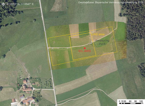
We collected airborne observations over a temperate grassland as part of the ScaleX 2016 field campaign (Wolf et al. 2017) at the Fendt site of the Terrestrial Observatories Network (TERENO) pre-Alpine observatory (Zacharias et al. 2011) in southern Germany. The site (DE-Fen) is equipped with a permanent EC station for water vapour, carbon dioxide, as well as energy flux measurements since 2010 (Zeeman et al. 2017). It includes a three-dimensional sonic anemometer (CSAT3, Campbell Scientific Inc., Logan, UT) and an infrared gas analyser (LI7500, LI-COR., Lincoln, NE). The station is located in a north–south-oriented valley in the foothills of the Bavarian Alps (47.833° N, 11.061° E; 595 m a.s.l.) with grassland being the prevailing land use with sporadic croplands (Brosy et al. 2017; Zeeman et al. 2017). In summer 2016, the grassland at the study site served as a meadow. Figure 1 shows an overview of the study area with the location of the EC station and the area of UAS-based thermal imaging. As shown in Figure 1, a dirt road and several scientific instruments were located within the UAS imaging area. The turbulent energy fluxes and corresponding flux footprints were computed in 30 min intervals (Mauder et al. 2013; Mauder and Foken 2015) and were combined with ancillary meteorological data listed in Table 1. The observed energy fluxes were adjusted in order to reach EB closure using a method that preserves the observed BR (Twine et al. 2000).

Table 1. Environmental observations at the study site and corresponding instrumentation.

Observed variable	Instrument
Air temperature	HMP45 (Vaisala, Vantaa, Finland)
Air pressure	WXT520 (Vaisala, Vantaa, Finland)
Surface temperature (1 min interval)	IR120 (Campbell Scientific Inc., Logan, UT)
Relative humidity	HMP45 (Vaisala, Vantaa, Finland)
Sensible and latent heat fluxes	CSAT3 (Campbell Scientific Inc., Logan, UT) LI7500 (LI-COR., Lincoln, NE)
Shortwave/longwave incoming/outgoing radiation	CNR 4 (Kipp&Zonen, Delft, The Netherlands)
Soil heat flux	HFP01-SC (Hukseflux, Delft, The Netherlands)
Wind speed	WXT520 (Vaisala, Vantaa, Finland)

Figure 1. Overview of the study area using an orthophoto (© Bayerische Vermessungsverwaltung – the Bavarian Agency for Surveying and Geoinformation) superimposed by an UAS-based RGB image acquired on 11 July at a flying altitude of 100 m. The red marker indicates the location of the EC tower. The solid yellow line sketches the area covered by the thermal imager for the flights at an altitude of 25 m. The dashed yellow line corresponds to the area covered with the flights at 100 m altitude. The exact extent of the thermal orthomosaic varied from flight to flight.

During the measurement campaign, farmers were managing the fields surrounding the EC station. After mowing, they distributed the cut grass over the field for drying and collected the dry grass the next day. Although UAS flights were conducted within a relatively short time window of 1 week, land-cover characteristics changed from standing high grass, to freshly cut grass to standing short grass between the single flights. While it was raining shortly before the observation period, it remained dry during the week of measurements.

2.1.2. UAS set-up and design of the flight campaign

An octocopter UAS (MikroKopter OktoXL, HiSystems GmbH, Moormerland, Germany) with a payload limit of 4 kg was used as a platform and was equipped with a commercially available digital RGB camera (Sony alpha 6000, Sony Corporation, Tokyo, Japan) and a thermal imager (Optris Pi Lightweight kit, Optris GmbH, Berlin, Germany). The Pi Lightweight kit with a weight of just 380 g consists of a small PC and a thermal camera (Optris Pi 400) and is designed for aerial thermography. The sensor detects thermal radiation in the spectral range from 7.5 to 13 µm and has a thermal sensitivity of 80 mK and accuracy of ±2.0°C. The optical resolution is 382 × 288 pixels with a field of view of 38° × 29° (f = 15 mm). The digital camera was triggered using the Sony PlayMemories Time-lapse Camera App, provided by the manufacturer. Focus, exposure, aperture, and ISO configurations were set manually before the flight and kept constant during the flight. Both cameras were mounted on a gimbal to allow for the collection of nadir-view LST images and were triggered every second during the whole flight. UAS flights were conducted along predefined waypoints covering the area around the EC station. Table 2 gives an overview of the flight characteristics.

Table 2. Overview of flight date, time, altitude, and covered area.

Flight no.	Date	Time (h:min)	Altitude (m)	Speed (m s^−1)	Area (ha)
1	5 July 2016	11:11–11:16	25	2	0.7
2	6 July 2016	13:11–13:16	25	2	0.64
3	6 July 2016	14:03–14:06	100	5	2.71
4	6 July 2016	15:04–15:09	25	2	0.78
5	7 July 2016	12:16–12:21	25	2	0.82
6	7 July 2016	16:41–16:46	25	2	0.72
7	8 July 2016	13:02–13:07	25	2	0.75
8	10 July 2016	13:16–13:21	25	2	1.55
9	11 July 2016	13:34–13:39	25	2	1.66
10	11 July 2016	17:00–17:04	100	5	5.85

The flight time is given in local time (UTC +2, CET DST).

Due to the close proximity of a glider plane airfield near the field site, flying altitude was restricted to 25 m for most of the conducted flights. Only for 2 days, where a flight coordinator was present at the field, flights up to an altitude of 100 m were made. Flying speed was set to 2 and 5 m s⁻¹ at 25 and 100 m altitude, respectively, in order to achieve a high degree of overlap between consecutive TIR images. The area covered with the thermal sensor varied between flights from 0.64 to 5.85 ha (see Table 2). The native resolution of the thermal imagery is around 5 and 20 cm for flights at 25 and 100 m altitude, respectively. The native resolution of the RGB imagery is higher with around 1 and 4 cm at 25 and 100 m flying altitude.

2.2. UAS image processing

For each flight a series of RGB and thermal images were recorded in 1 s intervals. The single images were combined into an RGB and thermal orthomosaic for each flight. Orthomosaics were generated using Agisoft PhotoScan Professional (Agisoft LLC). The software reconstructs a three-dimensional point cloud from overlapping single images with a technique called Structure from Motion (Westoby et al. 2012; Fonstad et al. 2013; Smith, Carrivick, and Quincey 2016). In the first step, image alignment, information from the GPS unit of the UAS was used as a first estimate of camera location and orientation. Once all images were aligned, camera locations were refined using ground control points that were derived from a high-resolution digital elevation model and an orthophoto available for the study site. After image alignment, a dense point cloud is generated that serves as basis for creating a digital elevation model as well as the orthomosaic. The same procedure was applied to the RGB and thermal imagery.

Both TSEB and the Triangle Method need information on vegetation properties. Thereto, two VIs were derived from the RGB orthomosaics. First, the Normalized Green-Red Difference Index (NGRDI) given in Equation (1) expresses the difference between the green and red bands divided by their sum (Pérez et al. 2000). At our study site, the discrimination between living green and dried dead vegetation, which was used for the determination of the fraction of green vegetation (f_g) in the TSEB model, was important since f_g was very heterogeneous over the field and changed in between flights because farmers were mowing the fields. Since the NGRDI did not separate these two groups satisfactorily, a second index was tested as model input. It is derived from the difference between the green and the blue bands divided by their sum (see Equation (2)) and is in the following abbreviated as NGBDI for Normalized Green-Blue Difference Index (Wang et al. 2015; Du and Noguchi 2017). Preliminary tests showed that this index better discriminates between the living and dead grass. Compared to the red and green bands, the blue band digital numbers showed larger differences between pixels with green and dead vegetation with lower values for green vegetation than for dead vegetation, which allowed also visually for the best discrimination between the two groups of the three available single bands.

(1) $\mathrm{N}\mathrm{G}\mathrm{R}\mathrm{D}\mathrm{I}=\frac{g-r}{g+r}$(1)

(2) $\mathrm{N}\mathrm{G}\mathrm{B}\mathrm{D}\mathrm{I}=\frac{g-b}{g+b},$(2)

where r, g, b are the red, green, and blue channel of the RGB image.

Green and dead vegetation pixels were discriminated in the high-resolution NGBDI maps (1 cm resolution) by setting a threshold on the NGBDI index. The threshold was set manually so that it yielded the best visual separation of the green from the dead vegetation. The fraction of green vegetation, f_g, was then derived as the ratio of the green and dead vegetation pixels (1 cm resolution) within each pixel of the coarser thermal imagery (5 cm resolution).

LAI and vegetation height images were derived from detailed land-use maps that were compiled during the field campaign. Vegetation heights were measured on several days during the field campaign in order to incorporate changes due to management operations between flights. LAI was measured with a plant canopy analyser (LAI2000, LI-COR., Lincoln, NE). Since a detailed study on vegetation properties at the experimental site in 2015 showed that the used plant canopy analyser overestimates LAI for this temperate grassland site by approximately 60% (pers. comm. M. Zeeman), the measured values were corrected accordingly. The obtained relationship between vegetation height and LAI agreed well with the 2015 results.

One aim of this study was to analyse the sensitivity of the models to the spatial resolution of the model imagery input. To this end, aggregates of 0.25, 0.50, 0.75, 1, 2.5, 5, 10, 15, and 30 m representing mean values over the corresponding number of pixels were generated from the images in their native resolution. An upper limit of 30 m was chosen since it corresponds to the highest spatial resolution that can be achieved from satellite imagery (Landsat 7 and 8) using data fusion and data-mining sharpeners (Gao et al. 2006; Gao et al. 2012).

2.3. TSEB

The TSEB model, developed by Norman, Kustas, and Humes (1995), belongs to the group of SEB models (Kalma, McVicar, and McCabe 2008). These models intend to derive latent heat flux as the residual term of the EB equation once all other components are known:

(3) $R_{\mathrm{n}}=\mathrm{L}\mathrm{E}+H+G,$(3)

where R_n is net radiation, H is sensible heat flux, LE is latent heat flux, and G is soil heat flux. In the presented form, Equation (3) excludes the effects of canopy heat storage and local advection since their contributions are assumed to be negligible.

In contrast to ‘big-leaf’ one-source models (Monteith 1965), the TSEB model partitions the surface temperatures as well as the energy fluxes into a soil and a canopy component and balances the energy budget for these components separately:

(4) $R_{\mathrm{n}\mathrm{s}}=\mathrm{L}{\mathrm{E}}_{\mathrm{s}}+H_{\mathrm{s}}+G$(4)

(5) $R_{\mathrm{n}\mathrm{c}}=\mathrm{L}{\mathrm{E}}_{\mathrm{c}}+H_{\mathrm{c}},$(5)

where subscripts ‘s’ and ‘c’ represent the soil and canopy flux component, respectively.

Component net radiation was calculated using the approach described in Xia et al. (2016) and Song et al. (2016), which is based on measurements of incoming radiation components, the component temperatures T_s and T_c, and information on surface properties such as albedo, transmittance through the canopy and emissivity. Soil heat flux was estimated as a function of soil net radiation following the approach proposed by Santanello and Friedl (2003), which accounts for the phase shift between the two quantities during daytime. The three parameters required for the method by Santanello and Friedl (2003) were set to A = 0.25 and B = 24 h and the phase shift was set to 3.5 h.

The measured radiometric surface temperature (T_r) is linked to the component temperatures via the fractional vegetation cover (f_c) at the sensor viewing angle Θ:

(6) $T_{\mathrm{r}}={\left[f_{\mathrm{c}}\left(\mathrm{\Theta }\right)T_{\mathrm{c}}^4+\left(1-f_{\mathrm{c}}\left(\mathrm{\Theta }\right)\right)T_{\mathrm{s}}^4\right]}^{\frac{1}{4}}.$(6)

For the investigated grassland site, f_c was uniformly set to a value of 0.9.

The component sensible heat fluxes are driven by a temperature gradient and are regulated by a transport resistances network:

(7) $H_{\mathrm{s}}=\rho c_{\mathrm{p}}\frac{T_{\mathrm{s}}-T_{\mathrm{A}\mathrm{C}}}{r_{\mathrm{s}}}$(7)

(8) $H_{\mathrm{c}}=\rho c_{\mathrm{p}}\frac{T_{\mathrm{c}}-T_{\mathrm{A}\mathrm{C}}}{r_{\mathrm{x}}}$(8)

(9) $H=H_{\mathrm{s}}+H_{\mathrm{c}}=\rho c_{\mathrm{p}}\frac{T_{\mathrm{A}\mathrm{C}}-T_{\mathrm{a}}}{r_{\mathrm{a}}},$(9)

where ρ is the air density, c_p is the specific heat of air at constant pressure, T_a is the air temperature at a reference level, r_s, r_x, and r_a are the resistances to heat transfer from the soil surface, canopy, and atmospheric surface layer, respectively, and T_AC is the air temperature within the canopy stand. The roughness lengths for momentum and heat required for the estimation of the resistances were set to 0.125 of the vegetation height. The series resistance network is described in Colaizzi et al. (2012), Kustas and Norman (1999), and Timmermans et al. (2007).

Initially LE_c and thus H_c are estimated using a Priestley–Taylor formulation (Priestley and Taylor 1972):

(10) $\mathrm{L}{\mathrm{E}}_{\mathrm{c}}=R_{\mathrm{n}\mathrm{c}}-H_{\mathrm{c}}={\alpha }_{\mathrm{P}\mathrm{T}}{f}_{\mathrm{g}}\frac{\mathrm{\Delta }}{\gamma +\mathrm{\Delta }}{R}_{\mathrm{n}\mathrm{c}},$(10)

where α_PT (set to 1.26) is the Priestley–Taylor coefficient, f_g is the fraction of green vegetation, Δ is the slope of the saturation water vapour–temperature curve, and γ is the psychrometric constant. With an initial value for H_c, estimates of T_c and T_s can be obtained from Equations (6) and (8), respectively. In the case that the vegetation is not transpiring at a potential rate, LE from the canopy will be overestimated by the Priestley–Taylor formulation at the expense of LE from the soil. This might lead to condensation from the soil (negative LE_s), which is unlikely during daytime conditions. Thus, α_PT is decreased incrementally and the set of equations is solved until no condensation from the soil occurs. Finally, all other EB components are updated accordingly to satisfy the EB equation. The TSEB model implemented in this study in based on the publicly available code provided in the ‘pyTSEB’ GitHub repository (latest available version: commit from 19 December 2016, https://github.com/hectornieto/pyTSEB/tree/ac3fe785ead3a9c4f09d773e00a9334f75f21fd0).

As mentioned before, TSEB solves the set of equations for each pixel independently from its surrounding pixels. Thus also aerodynamic resistances are calculated independently for each pixel. In the case of satellite remote-sensing imagery with relatively low spatial resolution, this is a valid assumption. However, in the case of UAS-based imagery with very high spatial resolution, this assumption might no longer be physically meaningful since aerodynamic resistance is governed by processes at larger scales. In order to investigate the effect of this independent treatment of neighbouring pixels, the model was run in two different configurations. In one configuration, despite the high resolution, all pixels were treated independently (as in the case of satellite imagery). In a second configuration, the resistances and net radiation components calculated in the model runs with input imagery with a spatial resolution of 30 m (see Section 2.2 for more detail) were plugged into the high-resolution model runs. In the latter configuration, the assumption of a large enough averaging volume for these variables is ensured. However, at the same time the use of a coarser grid resolution for these parameters results in artificial sharp edges that superimpose the spatial patterns derived at the finer grid resolution. The comparison of these two parameterizations aims at evaluating the effect of the high degree of freedom for the resistances and net radiation components in the case of the high-resolution input imagery on the spatially weighted mean fluxes as well as the spatial variability.

Required inputs for the TSEB model are radiometric surface temperature, information on land-cover properties such as fractional vegetation cover, leaf area index (LAI), vegetation height, and fraction of green vegetation. Additionally, meteorological data on air temperature, wind speed, water vapour pressure, and atmospheric pressure as well as incoming shortwave radiation are required.

LST images acquired with the UAS, maps of LAI, vegetation height and fraction of green vegetation (see Section 2.2 for the derivation of these maps) were used as spatially distributed inputs to the TSEB model. Meteorological data was available from the EC tower.

2.4. Triangle Method

In the Triangle Method the combination of LST and vegetation properties represents a diagnostic for the surface status and surface energy fluxes partitioning (Jiang and Islam 2001; Moran et al. 1994; Tomás et al. 2014). The triangle is formed by plotting surface temperature against a VI as a proxy for vegetation cover properties. Commonly, this VI is the normalized difference vegetation index (NDVI), but also other variables such as LAI or fractional vegetation cover were applied in the past (Jiang and Islam 2003; Nishida 2003; Tomás et al. 2014). The triangular form originates from the fact that the temperature range over bare soil and low vegetation cover is larger than for fully developed canopies. A central assumption in the Triangle Method is that given a large enough number of pixels representing the full range of fractional vegetation cover as well as soil moisture availability, sharp edges emerge in the surface temperature–VI space (Carlson 2007). The warm edge reflects conditions of no ET, whereas the cold edge represents the upper bound of ET for a given vegetation class (Jiang and Islam 2001). Jiang and Islam (2001) proposed a model to calculate EF and ET from a Priestley–Taylor formulation:

(11) $\mathrm{L}\mathrm{E}=\varphi \left(R_{\mathrm{n}}-G\right)\frac{\mathrm{\Delta }}{\gamma +\mathrm{\Delta }},$(11)

where ϕ is a complex effective parameter that incorporates the combined effects of the α_PT parameter and a surface wetness parameter. Equation (11) can be expressed as a function of EF:

(12) $\mathrm{E}\mathrm{F}=\frac{\mathrm{L}\mathrm{E}}{R_{\mathrm{n}}-G}=\varphi \frac{\mathrm{\Delta }}{\gamma +\mathrm{\Delta }}.$(12)

The range of ϕ is thus limited to ϕ_min = 0 (EF = 0) for conditions of no ET and ϕ_max = (γ + Δ)/Δ (EF = 1) for conditions of potential ET (Stisen et al. 2008). In order to assess ϕ for each pixel in the image, the warm and cold edges of the triangle have to be defined. The cold and warm edges are calculated using the ‘simple’ dry edge algorithm and the ‘mean’ wet edge algorithm as detailed in de Tomás et al. (2014). The surface temperature–VI space is split into bins based on the VI and for each bin the maximum and minimum temperature are determined. The selected bin size might vary with image resolution and is typically smaller (0.01) for higher resolution imagery and larger (0.05) for coarser resolution imagery (Tomás et al. 2014; Zhang et al. 2016). In this study, we test the performance of both bin sizes. T_min for the cold edge is the mean of the minimum T_r values from the 20 bins with the largest VI values. The warm edge is derived from a linear fit between the maximum T_r values and the corresponding VI bin value. In the case of the highest image resolution, the second hottest pixel instead of the hottest pixel (maximum) per VI bin was used for the derivation of the dry edge in order to reduce the effect of outliers. Having estimates for the cold and warm edge, ϕ_i for each pixel can be scaled between ϕ_max and ϕ_i,_min based on its relative position in the surface temperature space.

(13) ${\varphi }_i=\frac{T_{i,max}-T_i}{T_{i,max}-T_{i,min}}\left({\varphi }_{max}-{\varphi }_{i,min}\right)+{\varphi }_{i,min}.$(13)

While ϕ_max is constant for all VI bins, ϕ_min varies with VI (Stisen et al. 2008). EF in combination with an estimate of available energy (net radiation minus soil heat flux) allows for the calculation of ET rates. Since this method does not include a scheme for the estimation of available energy, the approach implemented in the third model evaluated in this study, the DATTUTDUT model, is adopted for the Triangle Method as well (the description of the DATTUTDUT model follows in the next section).

Typically, NDVI that combines information from the red and NIR spectral range is used as VI. Since our UAS set-up consisting of a thermal and a regular digital camera did not allow for the acquisition of data in the NIR spectral range, the applicability of other VIs relying solely on information from the red, green, and blue bands was tested. In this study, we used the UAS-based thermal images as well as maps of NGRDI and NGBDI (see Section 2.2 for the derivation of the VI maps) as model inputs for the Triangle Method. Since preliminary tests showed that a measuring truck permanently located at the study site (see Figure 1) affected the shape of the surface temperature–VI space, the measuring truck was masked in the input imagery for the estimation of the wet and dry edge.

2.5. DATTUTDUT

In contrast to contextual models that explore the surface temperature–VI space, the DATTUTDUT model proposed by Timmermans, Kustas, and Andreu (2015) estimates EF solely from surface temperature information. The rationale for the development of the DATUTDUT model is that more complex models in general rely on more input information and thus model estimates might become uncertain in regions where these data are not available or unreliable. The model interprets LST as a key indicator for the surface status. Assuming that the image scene contains the whole range of possible states, EF can be scaled between the extreme dry/hot pixels representing areas without ET and cold/wet pixels where ET is at its potential rate:

(14) $\mathrm{E}\mathrm{F}=\frac{\mathrm{L}\mathrm{E}}{\mathrm{L}\mathrm{E}+H}=\frac{\mathrm{L}\mathrm{E}}{R_{\mathrm{n}}-G}=\frac{T_{\mathrm{m}\mathrm{a}\mathrm{x}}-T_{\mathrm{r}}}{T_{\mathrm{m}\mathrm{a}\mathrm{x}}-T_{\mathrm{m}\mathrm{i}\mathrm{n}}},$(14)

where in the original paper T_max is taken as the hottest pixel, T_min is taken as the 0.5% quantile of surface temperature in the scene and T_r is the radiometric surface temperature for each pixel. In this study, the 99.99% quantile was taken as T_max instead of the hottest pixel.

In order to derive ET rates from the computed EF, estimates of R_n and G are needed. DATTUTDUT computes R_n similarly to EB models from the net shortwave and longwave radiation:

(15) $R_{\mathrm{n}}=\left(1-\alpha \right)R_{\mathrm{s}\mathrm{d}}+{ϵ}_{\mathrm{s}}{ϵ}_{\mathrm{a}}\sigma T_{\mathrm{a}}^4-{ϵ}_0\sigma T_{\mathrm{r}}^4,$(15)

where R_sd is incoming shortwave radiation, α is surface albedo, ε_s and ε_a are surface and atmospheric emissivity, T_a is air temperature, and σ is the Stefan–Boltzmann constant. The procedure for the derivation of net radiation described here and adopted from Timmermans, Kustas, and Andreu (2015) is also used for the Triangle Method.

To avoid the need for user inference, the DATTUTDUT model sets nominal values for ε_s (1.0) and ε_a (0.7). T_a is assumed to be equal to T_min. G is calculated as a fraction of R_n (Γ). In the DATTUTDUT model, Γ and α scale linearly with LST between 0.05 and 0.45 and between 0.05 and 0.25, respectively, with higher surface temperatures leading to higher factors as shown in Equations (16) and (17) (Equations (3) and (7) in Timmermans, Kustas, and Andreu 2015):

(16) $\alpha =0.05+0.2\left(\frac{T_{\mathrm{r}}-T_{\mathrm{m}\mathrm{i}\mathrm{n}}}{T_{\mathrm{m}\mathrm{a}\mathrm{x}}-T_{\mathrm{m}\mathrm{i}\mathrm{n}}}\right)$(16)

(17) $\mathrm{\Gamma }=0.05+0.4\left(\frac{T_{\mathrm{r}}-T_{\mathrm{m}\mathrm{i}\mathrm{n}}}{T_{\mathrm{m}\mathrm{a}\mathrm{x}}-T_{\mathrm{m}\mathrm{i}\mathrm{n}}}\right).$(17)

The DATTUTDUT model assumes clear-sky conditions and derives R_sd from Sun–Earth geometry relationships to minimize user interference and data requirements (Timmermans, Kustas, and Andreu 2015). However, since we conducted flights also under cloudy conditions, we use measured R_sd from the EC tower. Thus, R_sd and the UAS-based thermal imagery are the sole inputs to the model. Since the model otherwise runs fully automated, the user inference is limited to the generation of an orthomosaic of LST.

3. Results and discussion

We start the discussion of the results by analysing the effect of the spatial resolution of the input imagery on model estimates in Section 3.1. In Section 3.2 model estimates are compared to EC observations. In both sections, the presented results of the Triangle Method correspond to the model runs with the NGBDI as VI and the VI bin size set to 0.01. Regarding the parameterization of the resistance and radiative terms in the TSEB model, a comparison showed that almost no differences in the spatially weighted mean fluxes exist between the two tested setups (see Table 3). Thus, in both sections we only show the results of model runs for which the resistance and radiative terms were calculated on an individual pixel basis. A comparison of the two VIs is also presented in this section. For better readability, the Triangle Method will be abbreviated as TM in all figures. The spatial patterns and frequency distributions of modelled EF are discussed in Section 3.3.

Table 3. Difference statistics comparing model output of energy balance components as well as evaporative fraction from the TSEB, DATTUTDUT, and Triangle Method (TM) model with EC observations (closed with Bowen ratio method) in W m⁻².

	TSEB ind, res			DATTUTDUT			TM NGBDI, NGRDI
	Bias	MAE	RMSE	Bias	MAE	RMSE	Bias	MAE	RMSE
Rn (W m^−2)	−8	14	17	−34	44	51	−34	44	51
LE (W m^−2)	−13, −10	37, 38	50, 49	2	23	29	8, 0	27, 32	31, 34
H (W m^−2)	8, 6	31	49	6	30	37	−1, 7	41, 46	46, 52
G (W m^−2)	−4	18, 19	24	−41	50	55	−41	50	55
EF	0.01, 0.02	0.08	0.11	0.03	0.07	0.09	0.03, 0.00	0.09	0.10

Listed are the bias (Σ(O – M)/n), mean absolute error (MAE = Σ|O – M|/n), and root mean squared error (RMSE = [Σ(O – M)²/n]^1/2), where n is the sample size, O is the observed, and M is the modelled value. For the TSEB model, two values are given for the model runs with aerodynamic and radiative terms calculated at a 30 m grid (res) and independently for each pixel (ind). For the TM model, the two values refer to the model runs using either NGBDI or NGRDI as vegetation index. In the case that both parameterizations resulted in the same value, only one value is given for both.

3.1. Sensitivity of model estimates to the spatial resolution of the input imagery

UAS-based imaging campaigns allow for the acquisition of observations with high spatial resolution. In order to analyse the effect of the spatial resolution of the ET model input imagery, fluxes were computed for different image resolutions using the spatially aggregated remotely sensed observations of LST and vegetation properties. Xia et al. (2015) evaluated the performance of the TSEB and DATTUTDUT model over vineyards using aircraft-based remotely sensed observations. While they ran the DATTUTDUT model at the native pixel resolution (varying between 0.38 and 0.66 m for the thermal images), observations were spatially aggregated to 5 m resolution to create TSEB input fields. This resolution ensured that both an inter-row and vine row were sampled within each pixel, which is an integral part of the parameterization of the TSEB model. However, even though in the case of grassland the sampling of both soil and vegetation component within each pixel will be ensured at much higher resolution, model assumptions might still be violated if the input grid size becomes too fine. On the other hand, for contextual models a high image resolution is becoming more important as image domain becomes smaller (Long, Singh, and Scanlon 2012; Tomás et al. 2014). A large number of pixels should ensure a wide range of sampled vegetation cover and soil moisture states. In this study, we kept the image domain size constant and varied the spatial resolution of the imagery from the native resolution of 5 and 20 cm at 25 and 100 m flying altitude, respectively, to 30 m averages.

Figure 2 shows exemplarily the effect of the spatial resolution of the model input imagery on the modelled fluxes for three flights at different days for the Triangle Method, TSEB, and DATTUTDUT model. It depicts the modelled mean flux, which was spatially weighted according to the footprint weights, for each energy component as well as the corresponding standard deviation as a function of the input resolution (from coarse to high resolution from left to right). It is evident that the contextual models are highly sensitive to the input resolution, which is for the given domain size inversely proportional to the number of pixels available for scaling between the extreme wet/cold and dry/hot endmembers. For the DATTUTDUT model, latent heat flux estimates strongly vary with changes in the spatial resolution and show a tendency towards higher latent heat fluxes with higher spatial resolution of the inputs. The Triangle Method shows in general a similar albeit less pronounced behaviour, however, not as consistently over all flights (see Figure 2(h)). As is shown in Figure 3(a), the level of sensitivity varies with the parameterization of the wet/cold and dry/hot edge, i.e. the selected bin size. In comparison, the TSEB model shows a low sensitivity to the input resolution of the LST input data. Only on 5 July, when large areas of the field were covered with freshly mowed grass, which was spread over the field for drying, the high native resolution results in a significantly lower latent heat flux and a concomitant higher soil heat flux compared to the coarser input resolutions (see Figure 2(a)). For the native resolution imagery, 17% of all pixels have a fraction of green vegetation (f_g) of zero (for comparison: the share of pixels with a f_g of zero is only 3% for the second highest resolution of 0.25 m). In principle, the valid range for this parameter is 0 ≤ f_g ≤ 1 (Guzinski et al. 2013). However, for pixels with a f_g of zero the soil heat flux is increased significantly at the expense of the latent heat flux, which is set to zero. This reflects the model’s assumptions that no transpiration occurs from pixels with a f_g of zero and for pixels without transpiration also no evaporation from the soil occurs (Guzinski et al. 2015). The rational for this assumption is that if the Priestley–Taylor coefficient α falls below zero in the iterative process (meaning no transpiration from this pixel), this indicates very dry conditions under which no evaporation from the soil would occur. For the high level of disaggregation in the native resolution imagery with f_g values of zero, the modelled energy partitioning for these pixels results in a deterioration of the agreement with the observations as shown in Figure 3(a). However, alternatively, the model could be switched from a two-source to a one-source EB model, which does not partition the turbulent fluxes into a soil and canopy component, for pixels with a f_g of zero. Using this parameterization instead, still a decrease of the latent heat flux at the expense of increases in the sensible and soil heat flux could be observed for the native pixel resolution compared to the coarser resolution runs (not shown here). However, the effect of the high spatial resolution was clearly alleviated using the one-source approach for these pixels.

Figure 2. Change in modelled energy fluxes as well as surface temperature as a function of the resolution of the input imagery for three flights. Given are the mean (solid line) and the standard deviation (colour bands) of modelled energy components (a–i) and surface temperature (j–l) for the different input resolutions with input image resolution increasing from left to right. The flight date as well as time (h:min) is indicated above each subplot.

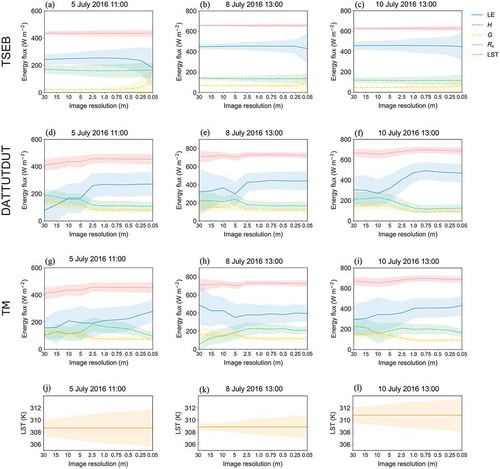
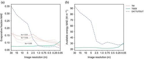
Figure 3. Mean absolute error (MAE) of the evaporative fraction (a) as well as available energy (b) as a function of the spatial resolution of the thermal and RGB input imagery for the TSEB, DATTUTDUT, as well as Triangle Method (TM) model. The DATTUTDUT and TM model incorporate the same scheme for the estimation of available energy. Image resolution increases from left to right. The selected bin size (VI bs) is a model parameter in the Triangle Method that affects the estimation of the cold/wet and dry/hot extremes. The EC measurements were closed using the Bowen ratio method.

As demonstrated by Figure 2, the TSEB model and the two contextual models show differences in flux variability with input resolution. While the variability of energy fluxes, as indicated by the standard deviation, increases with the spatial resolution in the TSEB model (as might be expected), the opposite occurs in the case of the two contextual models. The spatial averaging acts as a low-pass filter that in turn impacts the scaling of the EF and shifts the frequency histogram towards the extremes.

Figure 3 shows the variation of the mean absolute error (MAE) of EF and available energy with image resolution. Both contextual models estimate primarily EF and derive turbulent heat fluxes by multiplying the modelled EF value with estimates of available energy that are derived from surface temperature information and an estimate of shortwave incoming radiation. However, this simplistic method for the estimation of available energy is not explicitly linked to the two contextual models themselves and could be substituted by a more sophisticated modelling scheme if the required data is available. Thus, the use of EF instead of turbulent heat fluxes in Figure 3(a) places more emphasis on the effect of the spatial resolution on the model core assumptions and less on the correct estimation of available energy. In the case of the DATTUTDUT model, the MAE of EF decreases continuously between 30 and 1 m image resolution, then remains similar for all other model runs and reaches its minimum at the native image resolution. For the Triangle Method, the sensitivity to the spatial resolution of the input depends on the selected VI bin size in the definition of the wet/cold and dry/hot edge. While in the case of a VI bin size of 0.05 the MAE of EF is relatively constant over most of the input resolutions, a higher variability can be observed for a bin size of 0.01. However, for all displayed bin sizes the native resolution always leads to a low MAE.

According to Carlson (2007), the Triangle Method is able to yield EF estimates with a typical MAE of 0.1 and 0.2 (Jiang, Islam, and Carlson 2004). In our study, the MAE is below 0.2 for all image resolutions and falls below 0.1 regardless of the VI bin size only when using the highest image resolution. As already demonstrated in Figure 2, the TSEB model shows a low sensitivity to image resolution. The increase of the MAE of EF at the native resolution is a result of the energy partitioning for pixels with a f_g of zero as discussed before.

Figure 3(b) shows the MAE of available energy as a function of image resolution. Similar to EF, the TSEB model estimates available energy with little MAE for all image resolutions with a slight increase at the native image resolution. For the two contextual models, which both use the same scheme to model available energy, MAE first decreases rapidly with increasing resolution and then flattens out for higher resolutions.

In general, the sensitivity analysis of the model performance to image resolution shows that higher resolution leads to better EF estimates by the two contextual models even though a coarser bin size dampens the effect of spatial resolution in the case of the Triangle Method. Interestingly, the increase of input resolution below 1 m does only slightly affect the mean error of the DATTUTDUT model that uses solely the variability in LST for scaling between the minimum and maximum temperature. Thus, Figure 3(a) suggests that for the given study area and for resolutions higher than 1 m, estimates by the DATTUTDUT model are relatively insensitive to the exact image resolution. The VI bin size influences the effect of the spatial resolution in the Triangle Method. However, even though a low MAE was observed also for coarser resolutions, depending on the model parameterization (see Figure 3(a)), in general a higher input resolution leads to a more robust model performance. The preference of a high input resolution is also motivated by the better prediction of available energy with higher resolution inputs. For the single-pixel TSEB model, an effect of image resolution on modelled energy flux partitioning could be observed only in the case of the native image resolution. However, even at this very high resolution, a deterioration of flux estimates could be observed only for a share of pixels with very specific properties, namely a f_g of zero, that occurred predominantly on the day after mowing.

3.2. Comparison of model estimates and EC observations

In this section, we present a detailed comparison of model estimates and EC measurements. For the comparison, modelled spatially distributed fluxes were aggregated to a spatially weighted mean flux according to the estimated footprint of the EC measurements. As described in the previous section, the modelled fluxes vary with TIR and RGB image resolution with the sensitivity being more pronounced for the contextual models. Thus, the resolution that meets best the model’s assumptions and theoretical background was used for the comparison to the observations. In the case of the TSEB model, which is relatively insensitive to the image resolution, model outputs of the 0.5 m aggregates were used. For the grassland land cover, this resolution ensured the assumption of mixed pixels containing information of the soil and vegetation component for the vast majority of pixels. For the two contextual models, we used the native resolution of the imagery, which yields the largest number of pixels for the definition of the wet/cold and dry/hot edges for the Triangle Method and maximum and minimum surface temperatures for the DATTUTDUT model.

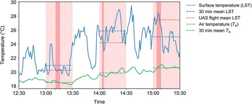
Figure 4 shows the comparison of the modelled and observed fluxes for each of the three models, where marker colours refer to the date and time of UAS-based data acquisition. Observed fluxes were closed using the BR method (Twine et al. 2000). Table 3 gives an overview of difference statistics summarizing the agreement of model results and observations. In general, all three models reproduce observed latent heat fluxes fairly well. In the case of the TSEB model, except for two flights that will be discussed in the following, the difference between observed and modelled latent heat fluxes is less than 50 W m⁻². For the two contextual models, the patterns of the agreement with the observations are very similar showing the same tendency to an over- or underestimation for the single flights. The similar behaviour of the contextual models is underlined by their high correlation coefficient especially for the latent heat fluxes given in Table 4. The difference to the observation exceeds 50 W m⁻² only once and twice for the Triangle Method and DATTUTDUT model, respectively. Soil heat flux estimates by the TSEB model agree clearly better with the observations, especially due to their small bias (less than 5 W m⁻²) in contrast to the two contextual models that systematically overestimate soil heat flux (both contextual models use the same scheme to model soil heat flux and net radiation). An exception is the flight on 11 July at 17:00 (local time) were net radiation was already low and the observed ratio of net radiation to soil heat flux (Γ) was high. Also in the case of net radiation, estimates by the TSEB model agree well with the observations. Here, the contextual models show a slight overestimation with higher values. However, it is worth mentioning that for the contextual models the soil heat flux and net radiation were modelled using a simplistic scheme described in Timmermans, Kustas, and Andreu (2015). In this approach, air temperature, vapour pressure, and albedo needed for the estimation of net radiation are derived from the LST information. The use of measured meteorological data led to a marginal improvement of modelled net radiation (reduction of MAE of net radiation from 44 to 35 W m⁻², not shown here), however, at the expense of higher input requirements. In general, the use of a more complex description of net radiation could improve turbulent flux estimates. However, since advantages of contextual models are the simple computation and low input requirements and user interference, the parameterization was kept in the described simplistic form. Since contextual models calculate EF by scaling between the endmember extremes and then use the calculated available energy (net radiation minus soil heat flux) to estimate turbulent heat fluxes, the accuracy of net radiation and soil heat flux estimates influences the model outputs of the turbulent heat fluxes. However, since the errors of both quantities are of the same magnitude, the effect on the available energy is comparatively low (Timmermans, Kustas, and Andreu 2015). Figure 4(e) shows the comparison of modelled and observed EF. For this quantity, all models perform comparably well. However, both contextual models cover a smaller range of EF values compared to the EC measurements and show relatively constant values for observed EF values below 0.70. All models underestimate the high observed EF close to unity for the late afternoon flight on 11 July at 17:00 (local time). It is worth mentioning that, as displayed in Figure 4, relatively high EF rates prevailed during the field campaign. Thus, no conditions of low EF linked to, e.g. water stress could be observed during the UAS campaign. In general, the TSEB model seems to better reproduce the variability in observed EF values; however, it shows larger deviations from the observations for two flights on 6 July. For both flights, the estimates by the two contextual models better match the observations. While TSEB overestimates EF at 14:00 (local time), it underestimates EF for a flight 1 h later. Figure 5 shows a time series of continuous (1 min resolution) surface temperature measurements from an infrared temperature sensor mounted at the EC tower and thus the variation of LST within half-hourly intervals over which turbulent heat fluxes are averaged. The dashed blue line represents the mean of these continuous measurements over half an hour indicated by the light red background. The darker red block within these half hours corresponds to the time period of the UAS flight. The dashed red line represents the mean LST over this shorter time span. It is evident that for both flights the difference between the mean LST during the UAS flight and the mean LST over the half hour for EC averaging is relatively large, with values of −1.7°C at 14:00 and +2.4°C at 15:00, respectively. Since air temperature does not fluctuate as much in the same time, the temperature gradient during the UAS flight is different to the gradient during the full half hour of EC flux averaging. Since this gradient builds the main driving force for energy partitioning in EB models, the TSEB model tends to an overestimation of EF compared to the EC measurement for the flight at 14:00 (local time), when the air-to-surface temperature gradient during the UAS flight was lower than the half-hour mean. For the flight at 15:00 the reverse happened and thus TSEB underestimates EF under these conditions. In both cases, the UAS-based LST measurements do not properly reflect the actual half-hour average circumstances and it might be that the TSEB model better represents the conditions during the actual UAS overpass than the two contextual models. However, a detailed analysis of flux conditions during the time of overpass would require EC measurements computed for shorter time intervals, e.g. 5 min. A 30 min interval is typically used for the computation of EC fluxes as this includes a sufficient part of time scales relevant for the computation of turbulent exchange between the surface and the atmosphere. However, future work might examine the agreement of model estimates with EC measurements computed for shorter time intervals, e.g. 5 min intervals, that correspond to the duration of the UAS surveys. For all other flights the offset between the mean LST during UAS overflight and the half-hour mean was less than 1.2°C. Rapid changes in LST were observed especially on days with scattered clouds. It is unlikely to get data from satellite platforms under these conditions; thus, the effect of LST and net radiation stability within half-hourly periods on the agreement between estimated and observed fluxes was not investigated in much detail (Kustas, Prueger, and Hipps 2002). However, UAS allow for data acquisition also under cloudy and overcast conditions with rapid changes in solar irradiation and as a result changes in surface temperature. When EB models are used under these conditions, special care has to be taken of the stability of surface and air temperature in the interpretation of the results of a comparison of modelled and observed fluxes. Hoffmann et al. (2016b) evaluated the TSEB model under cloudy and overcast conditions using fixed-wing UAS-based remotely sensed observations. They observed no significant differences in model performance compared to sunny conditions. However, they mention that scattered clouds during the flight (in their study a 20 min time span) will affect the generated thermal orthomosaic used in the EB model. In the present study, the flight time was shorter (around 5 min of data acquisition excluding starting and landing) and flights were timed to avoid abrupt changes between sunny and cloudy conditions during the flight as well as possible. Nevertheless, the variation of LST in the half hour of EC measurements led to a stronger disagreement between fluxes estimated by the TSEB model and EC observations on 6 July.

Table 4. Pearson correlation coefficients of latent heat flux (above the 1:1 line) and sensible heat flux (below the 1:1 line) for the TSEB, DATTUTDUT, and Triangle Method (TM).

	TSEB (ind)	TSEB (res)	DATT	TM (NGBDI)	TM (NGRDI)
TSEB (ind)	1	1	0.95	0.91	0.91
TSEB (res)	1	1	0.95	0.91	0.91
DATT	0.63	0.62	1	0.98	0.98
TVDI (GBI)	0.40	0.39	0.92	1	0.99
TVDI (NDI)	0.37	0.35	0.88	0.98	1

For the TSEB model, two values are given for the model runs with aerodynamic and radiative terms calculated at a 30 m grid (res) and independently for each pixel (ind). For the TM model, the two values refer to the model runs using either NGBDI or NGRDI as vegetation index.

Figure 4. Comparison of modelled and observed energy fluxes and evaporative fraction for the TSEB (0.5 m), DATTUTDUT (5 cm), and Triangle Method (TM) (5 cm) model. The observed data represents the EC data closed with the Bowen ratio method. The colours indicate the time and date of the UAS flights. The grey dashed line marks the 1:1 line.

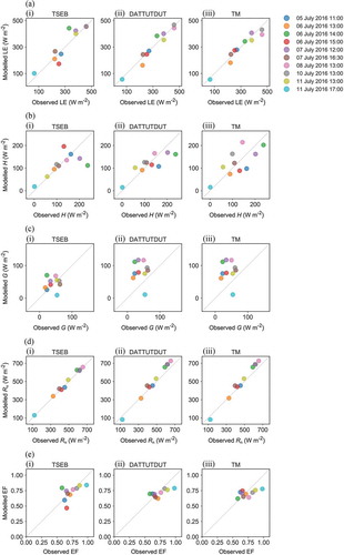
Figure 5. Time series of air (T_a) and surface temperature (LST) between 12:00 and 16:00 local time (UTC +2, CET DST) on 6 July 2016. The solid blue and green line represent 1 min interval measurements of LST (collected with an infrared temperature sensor mounted at the EC tower) and T_a, respectively. The light red blocks indicate half-hour intervals of EC averaging (always starting at full hours) that served as reference for modelled energy fluxes. The darker red shaded area delimits the time of UAS flights. The horizontal dashed lines mark the mean LST, the mean LST during UAS flights, and T_a in blue, red, and green, respectively.

Interestingly, this analysis showed that the simple DATTUTDUT model, even though only marginally, outperforms the more complex Triangle Method and TSEB model in the estimation of the latent heat flux and EF when only regarding the modelling statistics shown in Table 3. Prior inter-comparisons showed that in general flux estimates by the TSEB model are in better agreement with EC measurements over a wide range of environmental conditions and over homogeneous landscapes compared to contextual models (Choi et al. 2009; French, Hunsaker, and Thorp 2015; Timmermans et al. 2007; Xia et al. 2015; Colaizzi et al. 2012; Li et al. 2005). The slightly higher error statistics of the TSEB model in this study compared to the contextual models are a consequence of the larger deviations of the model results from the observations for the two flights on 6 July, a day with scattered clouds, as discussed above in detail. With regard to contextual models, Zipper and Loheide (2014) argued that the homogeneity of agricultural landscapes complicates the proper definition of the extreme limits at the field scale and limits the applicability of contextual models to transient dynamics in ET when the surface is neither totally bare nor fully covered by closed canopies. Even though the grassland at the study site represents a fairly homogeneous land cover, both contextual models performed well. The good performance of both contextual models in this study might be explained by the high disaggregation level of LST information that the high-resolution UAS-based imagery provides. The higher the resolution, the higher the chance for the simultaneous presence of the hydrological extremes within the image; a necessity for contextual models.

3.2.1. Comparison of two different VIs in the Triangle Method

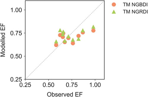
Since no information from the NIR range was available from the UAS-based imagery, the use of other VIs relying solely on information from the red, green, and blue range as input in the Triangle Method was tested. The results shown so far are based on a VI that is calculated in a similar manner as the NDVI but using information from the blue and green spectral range. Visible light VIs, such as the NGRDI, are often used to characterize vegetation if NIR information is lacking (Pérez et al. 2000; Meyer and Neto 2008; Raymond et al. 2005). Due to their low costs and low weight, consumer-grade true colour (RGB) digital cameras are particularly suitable for assessing green vegetation using UAS-based imaging systems (Torres-Sánchez et al. 2014; Saberioon et al. 2014; Hoffmann et al. 2016a; Goodbody et al. 2017; Jannoura et al. 2015). Rasmussen et al. (2016) evaluated the reliability of four VIs (ExG, NGRDI, NDVI, ENDVI) derived from consumer-grade RGB as well as CIR (colour-infrared) cameras mounted on UAS. Even though CIR cameras are sometimes recommended rather than RGB cameras, they found no clear advantage of CIR images and concluded that RGB cameras are powerful tools for assessing green vegetation. Hoffmann et al. (2016a) used the NGRDI based on UAS imagery to assess surface greenness of barley fields for the detection of crop water stress. In their study, they found a medium–strong correlation between the NGRDI and the NDVI and concluded that their results bode well for the use of the NGRDI as a greenness index. Figure 6 shows scatter plots of T_r versus the two tested VIs (NGRDI and NGBDI) as well as the calculated dry and wet edge for a bin size of 0.01 (solid line) and a bin size of 0.05 (dashed line) for three flights. While the NGBDI has a range comparable to the NDVI with most values between 0 and 0.8, the NGRDI has a significantly steeper dry edge with a smaller range of values (Raymond et al. 2005). In general, negative values are considered to be associated with soil pixels while positive values represent vegetated pixels. However, at our site a considerable share of pixels with negative NGRDI values were either freshly cut grass residuals or standing grass shortly after mowing. For the high-resolution input imagery, the effect of the selected bin size is relatively low in most cases as already indicated in Figure 3(a). Thus, even though the NDVI is the most commonly used VI for the Triangle Method, the form of the T_r–VI space presented in Figure 6 is promising for the further use of both NGRDI and NGBDI as VI if only true colour imagery is available. Despite the differences in the shape of the T_r–VI space of the two tested indices, both VI led to very similar EF estimates for all flights as demonstrated in Figure 7, which shows a comparison of EF modelled with the Triangle Method using the NGRDI and NGBDI, respectively.

Figure 6. Surface temperature (T_r)–vegetation index space for three flights for the NGBDI (a, c, e) and NGRDI (b, d, f). The solid and dashed lines represent the dry and wet edge for a selected bin size of 0.01 and 0.05, respectively.

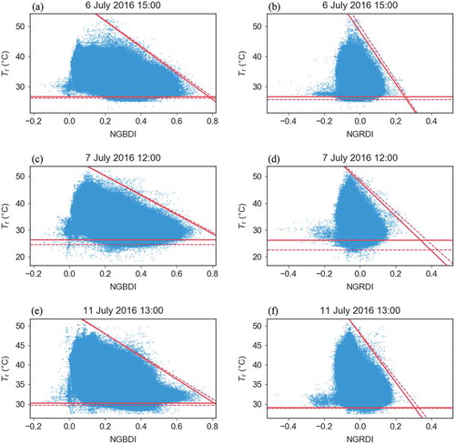
Figure 7. Comparison of model estimates of evaporative fraction (EF) by the Triangle Method (TM) based on the NGRDI (triangle) and NGBDI (circle) as vegetation index, respectively. Colours indicate the time and date of the UAS flights.

3.3. Comparison of patterns in modelled fluxes

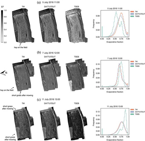
The comparison to the EC measurements focused on the representativeness of the modelled spatially weighted mean fluxes. Here, we analyse the distribution of modelled values using frequency histograms and maps of modelled EF. Figure 8 shows maps of instantaneous EF values as well as frequency histograms for three flights. As for the comparison to the EC measurements, the results shown here correspond to model computations with an image resolution of 0.5 m for the TSEB model and 5 cm for the two contextual models. For the TSEB model, Figure 8 shows the results for the model runs in which aerodynamic parameters were calculated on an individual pixel basis. While the frequency histograms of the two contextual models were in general very similar, the frequency histograms of the TSEB model showed a different EF distribution for some flights as indicated by Figures 8(a) and (c). For the flights on 5 July and 11 July, EF values differ significantly between the TSEB model and the contextual models. The histogram of the TSEB model shows a bimodal shape for both flights. EF values of zero result, as discussed before, from pixels with a fraction of green vegetation of zero. The bimodal shape of EF values modelled by the TSEB model is a consequence of the differences in vegetation height and LAI between the fields within the scene, which were mowed at different points in time (see Figure 8). In contrast, the two contextual models show a unimodal pattern for both flights that is shifted towards higher EF values compared to the TSEB model on 5 July and to lower values on 11 July. However, for both flights TSEB estimates agreed better with the EC observations. Figure 8(b) shows that for a flight for which all three models yielded similar mean EF values, also their frequency histograms agree well with each other.

Figure 8. Maps and frequency histograms of instantaneous evaporative fraction modelled by the TSEB (0.5 m), DATTUTDUT (5 cm), and Triangle Method (TM) (5 cm) for three flights.

The sensitivity analysis towards image resolution showed that the DATTUTDUT model performance was relatively independent of image resolution starting from 1 m resolution even though the number of pixels for scaling is decimated significantly (a factor of 400 from 5 cm resolution to 1 m). Figures 9(a) and (b) show frequency histograms of EF and LST for the DATTUTDUT model for model runs with 5 cm and 1 m, respectively, for 2 days. The effect of the higher input resolution is minor in most of the cases as indicated by Figure 9(b). Xia et al. (2015) observed a similar behaviour for the DATTUTDUT model for 5 m resolution and the native image resolution (varying between 0.38 and 0.66 m) over a vineyard. However, on 5 July a slight shift towards lower EF values and a trend towards a bimodal distribution as also shown by the TSEB model can be observed. This change in EF patterns results from a change in the frequency histogram of LST in the case of the high heterogeneity in LST observed for that day. Contrary to the DATTUTDUT model, the TSEB model keeps its bimodal shape for this flight even at a 5 cm resolution (not shown here).

Figure 9. Maps and frequency histograms of instantaneous evaporative fraction modelled by the DATTUTDUT model using input imagery with a resolution of 5 cm and 1 m (a, b), the Triangle Method (TM) using the NGBDI and NGRDI as vegetation index with a resolution of 5 cm (c), and the TSEB model using two different parameterizations of the aerodynamic properties with a resolution of 0.5 m (d, e). While in the ‘independent’ model runs in (d) and (e) aerodynamic properties were modelled for each pixel independently from the surrounding pixels, aerodynamic properties were calculated on a 30 m grid in the case of the ‘restricted’ model runs.

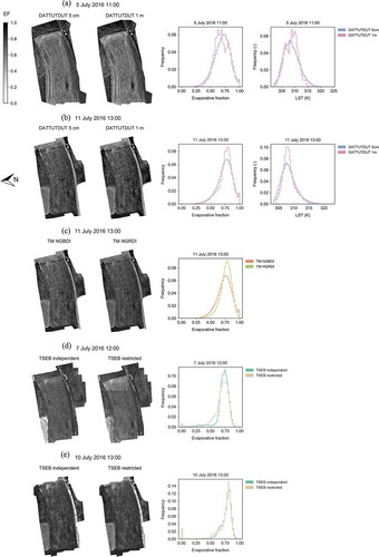
The two VIs tested for the Triangle Method, which yielded similar spatially weighted mean EF values, resulted also in similar spatial patterns of EF as exemplified in Figure 9(c). However, in general the NGBDI led to a slightly flatter histogram compared to the NGRDI.

Given the high resolution of the UAS-based imagery, the independent analysis of neighbouring pixels in the TSEB model may result in changes in the modelled resistances and radiative exchange processes within very short distances (in this case 0.5 m). However, boundary layer characteristic such as aerodynamic resistance is governed by processes on a larger scale and the independent treatment of pixels in the case of high-resolution imagery might introduce too many degrees of freedom for these parameters. Thus, two different parameterizations were tested. The two parameterizations (calculation of the resistances and net radiation terms on a 30 m grid and on a per-pixel basis) did not differ in the modelled mean fluxes; however, they show slight differences in the spatial distributions. As shown in Figure 9(d) the use of aerodynamic and radiative properties calculated on a coarser grid introduced artificial patterns in the modelled EF values when the differences of thermodynamic and vegetation properties between adjacent fields were high as on 7 July. At the same time, the restriction of the variability of these terms narrowed down the EF distribution. However, as depicted in Figure 9(e) for days with more transient changes in vegetation cover as on 10 July, no effect of the aerodynamic and net radiation parameterization on the spatial patterns could be observed. In general, the use of UAS and resulting high-resolution temperature data produce (boundary) conditions which might violate at least some of the assumption inherent in current ET modelling schemes commonly applied with satellite data. Even though in this study no significant differences between the two parameterizations could be observed, the use of high-resolution imagery might make adaptions in ET model setups necessary in order to comply with the model’s theoretical assumptions.

4. Conclusions

In this study, we used high-resolution UAS-based imagery in the visible and TIR spectrum in order to determine ET from a temperate grassland site. Three different ET modelling strategies were applied and their performances in reproducing field scale ET observations were evaluated for 10 UAS flights. Two of the applied models, the Triangle Method and DATTUTDUT model, belong to the group of contextual models that estimate EF by scaling the whole scene between the extreme endmembers of zero and potential ET. The third model applied in this study, the TSEB model, implements a more physically based two-source formulation that solves the EB equation for each individual pixel and explicitly treats energy and radiation exchanges with the atmosphere separately for the soil and canopy component.

Given that most TIR-based ET algorithms have been developed for satellite imagery with coarser resolution but larger areal extent compared to UAS-based imagery, the effect of the high spatial resolution of the input imagery on model results was studied in detail. For the DATTUTDUT model, the agreement with the observations significantly improved with increasing image resolution. The effect of image resolution on the performance of the Triangle Method was less clear and varied with the model parameterization, i.e. the selected bin size. However, the native resolution always led to the lowest MAE value regardless of model parameterization. The TSEB model showed the least sensitivity to input resolution of all three models. Since the TSEB model uses a more physically based formulation of the EB at the surface and, unlike contextual models, does not rely on the proper definition of extreme endmembers, it is more robust with respect to a varying image resolution. Only under very specific conditions shortly after mowing, when a considerable fraction of pixels in the UAS-based imagery had a fraction of green vegetation of zero, a limited deterioration of the agreement between the modelled energy fluxes and the EC observations could be observed for the TSEB model using the native image resolution.

The comparison of model estimates of ET and EF to the EC observations showed that all three models are able to reproduce the observations with comparable accuracy with a MAE of ET of 37, 27, and 23 W m⁻² for the TSEB model, Triangle Method, and DATTUTDUT model, respectively. The results of the two contextual models were similar for most of the flights. In the case of the Triangle Method, both tested VIs using information from the green and blue band (NGBDI) and the green and red band (NGRDI), respectively, yielded similar flux estimates for all flights.

The TSEB model performed best in reproducing measured net radiation and soil heat flux. The two contextual models use a simplistic scheme to model both quantities and showed an overestimation of soil heat flux and a slight overestimation of high net radiation values. In the present study, the errors in both quantities tended to cancel out each other in the calculation of the available energy and thus had a minor effect on modelled ET. However, this tendency might not hold for other locations or meteorological conditions.

The TSEB model showed higher discrepancies from the observed EF and ET values compared to the two contextual models for two flights. In both cases, cloudy conditions with strong fluctuations in surface temperature and thus gradients between the surface and air prevailed. Consequently, conditions during the UAS flight deviated from the average conditions during the half hour of EC averaging. Since the surface-to-air temperature gradient is the main driver in the TSEB model, the agreement between modelled and observed fluxes deteriorated under these conditions.

Our study showed that ET estimates of the simple DATTUTDUT model are in good agreement with the observations. This result is especially promising in view of possible routine near-real-time ET monitoring applications since the DATTUTDUT model requires no other than the LST information to model EF and, in the case of cloudy conditions, an estimate of shortwave incoming radiation to derive ET estimates from the modelled EF. However, in contrast to the DATTUTDUT model, the TSEB model can provide energy flux estimates for the canopy and soil component separately that might suit further interests for agricultural management and water management. Thus, as already suggested by Xia et al. (2015) the development of a hybrid methodology that integrates a very simple ET model (DATTUTDUT) and a more physically based ET model (TSEB) could be a possible next step towards routine high-resolution ET monitoring.

For the investigated grassland site, all three models proved to be suitable for mapping spatially distributed energy fluxes at the field scale using the UAS-based imagery. However, further experiments at different sites in different climates are required to make general statements about the applicability of these models at the field scale. The applied low-cost UAS system operated at low altitudes proved suitable for obtaining the required spatially distributed model input data. Thus, the results of this study support the applicability of UAS for field scale ET monitoring.

Acknowledgements

We thank the Scientific Team of ScaleX Campaign 2016 for their contribution. Many thanks to Matthias Mauder for providing the EC footprints and Hector Nieto for making the TSEB code freely available via github/pytseb. We are particularly grateful for the assistance and support given by Frederik Kratzert during the UAS field campaign. We would like to thank the editor and three anonymous reviewers for their insightful comments during the review process.

Disclosure statement

No potential conflict of interest was reported by the authors.

Additional information

Funding

This study was supported by the Austrian Science Fund (FWF) through funding of the CAOS (Catchments as Organised Systems) Research Unit [I 2142-N29]. Matthias Zeeman was supported by the German Research Foundation [DFG; project ZE1006/2-1]. The TERENO-preAlpine Observatory infrastructure is funded by the Helmholtz Association and the Federal Ministry of Education and Research.

References

- Allen, R., M. Tasumi, and R. Trezza. 2007. “Satellite-Based Energy Balance for Mapping Evapotranspiration with Internalized Calibration (Metric)—Model.” Journal of Irrigation and Drainage Engineering 133 (4): 380–394. doi:10.1061/(ASCE)0733-9437(2007)133:4(380).
- Anderson, M. C., J. M. Norman, G. R. Diak, W. P. Kustas, and J. R. Mecikalski. 1997. “A Two-Source Time-Integrated Model for Estimating Surface Fluxes Using Thermal Infrared Remote Sensing.” Remote Sensing Of Environment 60 (2): 195–216. doi:10.1016/s0034-4257(96)00215-5.
- Anderson, M. C., J. M. Norman, J. R. Mecikalski, J. A. Otkin, and W. P. Kustas. 2007. “A Climatological Study of Evapotranspiration and Moisture Stress across the Continental United States Based on Thermal Remote Sensing: 2. Surface Moisture Climatology.” Journal of Geophysical Research: Atmospheres 112: 1–13. doi:10.1029/2006JD007507.
- Anderson, M. C., W. P. Kustas, J. M. Norman, C. R. Hain, J. R. Mecikalski, L. Schultz, M. P. González-Dugo, et al. 2011. “Mapping Daily Evapotranspiration at Field to Continental Scales Using Geostationary and Polar Orbiting Satellite Imagery.” Hydrology and Earth System Sciences 15: 223–239. doi:10.5194/hess-15-223-2011.
- Bastiaanssen, W. G. M., E. J. M. Noordman, H. Pelgrum, G. Davids, B. P. Thoreson, and R. G. Allen. 2005. “SEBAL Model with Remotely Sensed Data to Improve Water-Resources Management under Actual Field Conditions.” Journal of Irrigation and Drainage Engineering 131 (1): 85–93. doi:10.1061/(ASCE)0733-9437(2005)131:1(85).
- Berni, J. A. J., P. J. Zarco-Tejada, L. Suárez, and E. Fereres. 2009. “Thermal and Narrowband Multispectral Remote Sensing for Vegetation Monitoring from an Unmanned Aerial Vehicle.” IEEE Transactions on Geoscience and Remote Sensing 47 (3): 722–738. doi:10.1109/TGRS.2008.2010457.
- Bhattarai, N., K. Mallick, N. A. Brunsell, G. Sun, and M. Jain. 2018. “Regional Evapotranspiration from Image-Based Implementation of the Surface Temperature Initiated Closure (STIC1. 2) Model and Its Validation across an Aridity Gradient in the Conterminous United.” Hydrology and Earth System Sciences 22: 2311–2341. doi:10.5194/hess-2017-535.
- Boegh, E., K. Schelde, and H. Soegaard. 2000. “Estimating Transpiration Rates in a Danish Agricultural Area Using Landsat Thermal Mapper Data.” Physics and Chemistry of the Earth, Part B: Hydrology, Oceans and Atmosphere 25 (7–8): 685–689. doi:10.1016/S1464-1909(00)00085-X.
- Brenner, C., C. E. Thiem, H.-D. Wizemann, M. Bernhardt, and K. Schulz. 2017. “Estimating Spatially Distributed Turbulent Heat Fluxes from High-Resolution Thermal Imagery Acquired with a UAV System.” International Journal of Remote Sensing 1–24. doi:10.1080/01431161.2017.1280202.
- Brosy, C., K. Krampf, M. Zeeman, B. Wolf, W. Junkermann, K. Schäfer, S. Emeis, and H. Kunstmann. 2017. “Simultaneous Multicopter-Based Air Sampling and Sensing of Meteorological Variables.” Atmospheric Measurement Techniques 10 (8): 2773–2784. doi:10.5194/amt-10-2773-2017.
- Cammalleri, C., M. C. Anderson, F. Gao, C. R. Hain, and W. P. Kustas. 2014. “Mapping Daily Evapotranspiration at Field Scales over Rainfed and Irrigated Agricultural Areas Using Remote Sensing Data Fusion.” Agricultural and Forest Meteorology 186: 1–11. doi:10.1016/j.agrformet.2013.11.001.
- Candiago, S., F. Remondino, M. De Giglio, M. Dubbini, and M. Gattelli. 2015. “Evaluating Multispectral Images and Vegetation Indices for Precision Farming Applications from UAV Images.” Remote Sensing 7 (4): 4026–4047. doi:10.3390/rs70404026.
- Carlson, T. 2007. “An Overview of the ‘Triangle Method’ for Estimating Surface Evapotranspiration and Soil Moisture from Satellite Imagery.” Sensors 7 (8): 1612–1629. doi:10.3390/s7081612.
- Chirouze, J., G. Boulet, L. Jarlan, R. Fieuzal, J. C. Rodriguez, J. Ezzahar, S. Er-Raki, et al. 2014. “Intercomparison of Four Remote-Sensing-Based Energy Balance Methods to Retrieve Surface Evapotranspiration and Water Stress of Irrigated Fields in Semi-Arid Climate.” Hydrology and Earth System Sciences 18 (3): 1165–1188. doi:10.5194/hess-18-1165-2014.
- Choi, M., W. P. Kustas, M. C. Anderson, R. G. Allen, L. Fuqin, and J. H. Kjaersgaard. 2009. “An Intercomparison of Three Remote Sensing-Based Surface Energy Balance Algorithms over a Corn and Soybean Production Region (Iowa, U.S.) During SMACEX.” Agricultural and Forest Meteorology 149 (12): 2082–2097. doi:10.1016/j.agrformet.2009.07.002.
- Cleugh, H. A., R. Leuning, M. Qiaozhen, and S. W. Running. 2007. “Regional Evaporation Estimates from Flux Tower and MODIS Satellite Data.” Remote Sensing of Environment 106: 285–304. doi:10.1016/j.rse.2006.07.007.
- Colaizzi, P. D., W. P. Kustas, M. C. Anderson, N. Agam, J. A. Tolk, S. R. Evett, T. A. Howell, P. H. Gowdaand S.A. O’Shaughnessy. 2012. “Two-Source Energy Balance Model Estimates of Evapotranspiration Using Component and Composite Surface Temperatures.” Advances in Water Resources 50: 134–151. Elsevier Ltd. doi:10.1016/j.advwatres.2012.06.004.
- Du, M., and N. Noguchi. 2017. “Monitoring of Wheat Growth Status and Mapping of Wheat Yield’s within-Field Spatial Variations Using Color Images Acquired from UAV-Camera System.” Remote Sensing 9: 3. doi:10.3390/rs9030289.
- Foken, T. 2008. Micrometeorology. Micrometeorology. Verlag, Berlin, Heidelberg, Germany: Springer-Verlag, Berlin, Heidelberg. doi:10.1007/978-3-540-74666-9.
- Fonstad, M. A., J. T. Dietrich, B. C. Courville, J. L. Jensen, and P. E. Carbonneau. 2013. “Topographic Structure from Motion: A New Development in Photogrammetric Measurement.” Earth Surface Processes and Landforms 38 (4): 421–430. doi:10.1002/esp.3366.
- French, A. N., D. J. Hunsaker, and K. R. Thorp. 2015. “Remote Sensing of Evapotranspiration over Cotton Using the TSEB and METRIC Energy Balance Models.” Remote Sensing of Environment 158: 281–294. Elsevier B.V. doi:10.1016/j.rse.2014.11.003.
- Gao, F., J. Masek, M. Schwaller, and F. Hall. 2006. “On the Blending of the MODIS and Landsat ETM + Surface Reflectance.” IEEE Transactions on Geoscience and Remote Sensing 44 (8): 2207–2218. doi:10.1109/TGRS.2006.872081.
- Gao, F., M. C. Anderson, W. P. Kustas, and Y. Wang. 2012. “Simple Method for Retrieving Leaf Area Index from Landsat Using MODIS Leaf Area Index Products as Reference.” Journal of Applied Remote Sensing 6 (1): 63554. doi:10.1117/1.JRS.6.063554.
- Gillies, R. R., and T. N. Carlson. 1995. “Thermal Remote Sensing of Surface Soil Water Content with Partial Vegetation Cover for Incorporation into Climate Models.” Journal of Applied Meteorology 34: 745–756. doi:10.1175/1520-0450(1995)034<0745:TRSOSS>2.0.CO;2.
- Gillies, R. R., W. P. Kustas, and K. S. Humes. 1997. “A Verification of The’triangle’method for Obtaining Surface Soil Water Content and Energy Fluxes from Remote Measurements of the Normalized Difference Vegetation Index (NDVI) and Surface E.” International Journal of Remote Sensing 18 (15): 3145–3166. doi:10.1080/014311697217026.
- Goodbody, T. R. H., N. C. Coops, T. Hermosilla, P. Tompalski, and P. Crawford. 2017. “Assessing the Status of Forest Regeneration Using Digital Aerial Photogrammetry and Unmanned Aerial Systems.” International Journal of Remote Sensing 1–19. doi:10.1080/01431161.2017.1402387.
- Guzinski, R., H. Nieto, S. Stisen, and R. Fensholt. 2015. “Inter-Comparison of Energy Balance and Hydrological Models for Land Surface Energy Flux Estimation over a Whole River Catchment.” Hydrology and Earth System Sciences Discussions 19: 2017–2036. doi:10.5194/hess-19-2017-2015.
- Guzinski, R., M. C. Anderson, W. P. Kustas, H. Nieto, and I. Sandholt. 2013. “Using a Thermal-Based Two Source Energy Balance Model with Time-Differencing to Estimate Surface Energy Fluxes with Day-Night MODIS Observations.” Hydrology and Earth System Sciences 17 (7): 2809–2825. doi:10.5194/hess-17-2809-2013.
- Hoffmann, H., H. Nieto, R. Jensen, R. Guzinski, P. Zarco-Tejada, and T. Friborg. 2016b. “Estimating Evaporation with Thermal UAV Data and Two-Source Energy Balance Models.” Hydrology and Earth System Sciences 20 (2): 697–713. doi:10.5194/hess-20-697-2016.
- Hoffmann, H., R. Jensen, A. Thomsen, H. Nieto, J. Rasmussen, and T. Friborg. 2016a. “Crop Water Stress Maps for an Entire Growing Season from Visible and Thermal UAV Imagery.” Biogeosciences 13 (24): 6545–6563. doi:10.5194/bg-13-6545-2016.
- Jannoura, R., K. Brinkmann, D. Uteau, C. Bruns, and R. G. Joergensen. 2015. “Monitoring of Crop Biomass Using True Colour Aerial Photographs Taken from a Remote Controlled Hexacopter.” Biosystems Engineering 129: 341–351. Elsevier Ltd. doi:10.1016/j.biosystemseng.2014.11.007.
- Jiang, L., and S. Islam. 2001. “Estimation of Surface Evaporation Map over Southern Great Plains Using Remote Sensing Data.” Water Resources Research 37 (2): 329–340. doi:10.1029/2000WR900255.
- Jiang, L., and S. Islam. 2003. “An Intercomparison of Regional Latent Heat Flux Estimation Using Remote Sensing Data.” International Journal of Remote Sensing 24 (11): 2221–2236. doi:10.1080/01431160210154821.
- Jiang, L., S. Islam, and T. Carlson. 2004. “Uncertainties in Latent Heat Flux Measurements and Estimation: Implications for Using a Simplified Approach with Remote Sensing Data.” Canadian Journal of Remote Sensing 30 (5): 769–787. doi:10.5589/m04-038.
- Kalma, J. D., T. R. McVicar, and M. F. McCabe. 2008. “Estimating Land Surface Evaporation: A Review of Methods Using Remotely Sensed Surface Temperature Data.” Surveys in Geophysics 29 (4–5): 421–469. doi:10.1007/s10712-008-9037-z.
- Kustas, W. P., J. G. Alfieri, M. C. Anderson, P. D. Colaizzi, J. H. Prueger, S. R. Evett, C. M. U. Neale, et al. 2012. “Evaluating the Two-Source Energy Balance Model Using Local Thermal and Surface Flux Observations in a Strongly Advective Irrigated Agricultural Area.” Advances in Water Resources 50: 120–133. Elsevier Ltd. doi:10.1016/j.advwatres.2012.07.005.
- Kustas, W. P., J. H. Prueger, and L. E. Hipps. 2002. “Impact of Using Different Time-Averaged Inputs for Estimating Sensible Heat Flux of Riparian Vegetation Using Radiometric Surface Temperature.” Journal of Applied Meteorology 41 (3): 319–332. doi:10.1175/1520-0450(2002)041<0319:IOUDTA>2.0.CO;2.
- Kustas, W. P., and J. M. Norman. 1999. “Evaluation of Soil and Vegetation Heat Flux Predictions Using a Simple Two-Source Model with Radiometric Temperatures for Partial Canopy Cover.” Agricultural and Forest Meteorology 94 (1): 13–29. doi:10.1016/S0168-1923(99)00005-2.
- Kustas, W. P., and M. Anderson. 2009. “Advances in Thermal Infrared Remote Sensing for Land Surface Modeling.” Agricultural and Forest Meteorology 149: 2071–2081. doi:10.1016/j.agrformet.2009.05.016.
- Lelong, C. C. D., P. Burger, G. Jubelin, B. Roux, S. Labbé, and F. Baret. 2008. “Assessment of Unmanned Aerial Vehicles Imagery for Quantitative Monitoring of Wheat Crop in Small Plots.” Sensors 8 (5): 3557–3585. doi:10.3390/s8053557.
- Li, F., W. P. Kustas, J. H. Prueger, C. M. U. Neale, and T. J. Jackson. 2005. “Utility of Remote Sensing Based Two-Source Energy Balance Model under Low and High Vegetation Cover Conditions.” Journal of Hydrometeorology 6: 878–891. doi:10.1175/JHM464.1.
- Liebethal, C., and T. Foken. 2007. “Evaluation of Six Parameterization Approaches for the Ground Heat Flux.” Theoretical and Applied Climatology 88 (1–2): 43–56. doi:10.1007/s00704-005-0234-0.
- Link, J., D. Senner, and W. Claupein. 2013. “Developing and Evaluating an Aerial Sensor Platform (ASP) to Collect Multispectral Data for Deriving Management Decisions in Precision Farming.” Computers and Electronics in Agriculture 94: 20–28. Elsevier B.V. doi:10.1016/j.compag.2013.03.003.
- Long, D., V. P. Singh, and B. R. Scanlon. 2012. “Deriving Theoretical Boundaries to Address Scale Dependencies of Triangle Models for Evapotranspiration Estimation.” Journal of Geophysical Research Atmospheres 117 (5): 1–17. doi:10.1029/2011JD017079.
- Mauder, M., M. Cuntz, C. Drüe, A. Graf, C. Rebmann, H. P. Schmid, M. Schmidt, and R. Steinbrecher. 2013. “A Strategy for Quality and Uncertainty Assessment of Long-Term Eddy-Covariance Measurements.” Agricultural and Forest Meteorology 169: 122–135. Elsevier B.V. doi:10.1016/j.agrformet.2012.09.006.
- Mauder, M., and T. Foken. 2015. “Eddy-Covariance Software TK3.” Zenodo. doi:10.5281/zenodo.20349.
- McMahon, T. A., M. C. Peel, L. Lowe, R. Srikanthan, and T. R. McVicar. 2013. “Estimating Actual, Potential, Reference Crop and Pan Evaporation Using Standard Meteorological Data: A Pragmatic Synthesis.” Hydrology and Earth System Sciences 17: 1331–1363. doi:10.5194/hess-17-1331-2013.
- Meyer, G. E., and J. C. Neto. 2008. “Verification of Color Vegetation Indices for Automated Crop Imaging Applications.” Computers and Electronics in Agriculture 63 (2): 282–293. doi:10.1016/j.compag.2008.03.009.
- Monteith, J. L. 1965. “Evaporation and Environment.” Symposia of the Society for Experimental Biology 19: 205–234.
- Moran, M. S., T. R. Clarke, Y. Inoue, and A. Vidal. 1994. “Estimating Crop Water Deficit Using the Relation between Surface-Air Temperature and Spectral Vegetation Index.” Remote Sensing of Environment 49 (3): 246–263. doi:10.1016/0034-4257(94)90020-5.
- Morillas, L., M. Garcia, H. Nieto, L. Villagarcia, I. Sandholt, M. P. Gonzalez-Dugo, P. J. Zarco-Tejada, and F. Domingo. 2013. “Using Radiometric Surface Temperature for Surface Energy Flux Estimation in Mediterranean Drylands from a Two-Source Perspective.” Remote Sensing of Environment 136: 234–246. doi:10.1016/j.rse.2013.05.010.
- Murray, T., and A. Verhoef. 2007. “Moving Towards a More Mechanistic Approach in the Determination of Soil Heat Flux from Remote Measurements. II. Diurnal Shape of Soil Heat Flux.” Agricultural and Forest Meteorology 147 (1–2): 88–97. doi:10.1016/j.agrformet.2007.06.009.
- Nishida, K. 2003. “An Operational Remote Sensing Algorithm of Land Surface Evaporation.” Journal of Geophysical Research 108 (D9). doi:10.1029/2002JD002062.
- Norman, J. M., and F. Becker. 1995. “Terminology in Thermal Infrared Remote Sensing of Natural Surfaces.” Remote Sensing Reviews 12 (3–4): 159–173. doi:10.1080/02757259509532284.
- Norman, J. M., W. P. Kustas, J. H. Prueger, and G. R. Diak. 2000. “Surface Flux Estimation Using Radiometric Temperature: A Dual-Temperature-Difference Method to Minimize Measurement Errors.” Water Resources Research 36 (8): 2263–2274. doi:10.1029/2000WR900033.
- Norman, J. M., W. P. Kustas, and K. S. Humes. 1995. “A Two-Source Approach for Estimating Soil and Vegetation Energy Fluxes in Observations of Directional Radiometric Surface Temperature.” Agricultural and Forest Meteorology 77 (3–4): 263–293. doi:10.1016/0168-1923(95)02265-Y.
- Ortega-Farías, S., S. Ortega-Salazar, T. Poblete, A. Kilic, R. Allen, C. Poblete-Echeverría, L. Ahumada-Orellana, M. Zuñiga, and S. Daniel. 2016. “Estimation of Energy Balance Components over a Drip-Irrigated Olive Orchard Using Thermal and Multispectral Cameras Placed on a Helicopter-Based Unmanned Aerial Vehicle (UAV).” Remote Sensing 8 (8): 638. doi:10.3390/rs8080638.
- Ortega-Farías, S., S. Ortega-Salazar, T. Poblete, C. Poblete-Echeverría, M. Zúñiga, D. Sepúlveda-Reyes, A. Kilic, and R. Allen. 2017. “Estimation of Olive Evapotranspiration Using Multispectral and Thermal Sensors Placed aboard an Unmanned Aerial Vehicle.” Acta Horticulturae 1150: 1–8. doi:10.17660/ActaHortic.2017.1150.1.
- Pérez, A. J., F. López, J. V. Benlloch, and S. Christensen. 2000. “Colour and Shape Analysis Techniques for Weed Detection in Cereal Fields.” Computers and Electronics in Agriculture 25 (3): 197–212. doi:10.1016/S0168-1699(99)00068-X.
- Priestley, C. H. B., and R. J. Taylor. 1972. “On the Assessment of Surface Heat Flux and Evaporation Using Large-Scale Parameters.” Monthly Weather Review 100 (2): 81–92. doi:10.1175/1520-0493(1972)100<0081:OTAOSH>2.3.CO;2.
- Rasmussen, J., G. Ntakos, J. Nielsen, J. Svensgaard, R. N. Poulsen, and S. Christensen. 2016. “Are Vegetation Indices Derived from Consumer-Grade Cameras Mounted on UAVs Sufficiently Reliable for Assessing Experimental Plots?” European Journal of Agronomy 74: 75–92. Elsevier B.V. doi:10.1016/j.eja.2015.11.026.
- Raymond, H. E., M. Cavigelli, C. S. T. Daughtry, J. E. McMurtrey, and C. L. Walthall. 2005. “Evaluation of Digital Photography from Model Aircraft for Remote Sensing of Crop Biomass and Nitrogen Status.” Precision Agriculture 6 (4): 359–378. doi:10.1007/s11119-005-2324-5.
- Reineman, B. D., L. Lenain, N. M. Statom, and W. Kendall Melville. 2013. “Development and Testing of Instrumentation for UAV-Based Flux Measurements within Terrestrial and Marine Atmospheric Boundary Layers.” Journal of Atmospheric and Oceanic Technology 30 (7): 1295–1319. doi:10.1175/JTECH-D-12-00176.1.
- Saberioon, M. M., M. S. M. Amin, A. R. Anuar, A. Gholizadeh, A. Wayayok, and S. Khairunniza-Bejo. 2014. “Assessment of Rice Leaf Chlorophyll Content Using Visible Bands at Different Growth Stages at Both the Leaf and Canopy Scale.” International Journal of Applied Earth Observation and Geoinformation 32 (1): 35–45. Elsevier B.V. doi:10.1016/j.jag.2014.03.018.
- Santanello, J. A., and M. A. Friedl. 2003. “Diurnal Covariation in Soil Heat Flux and Net Radiation.” Journal of Applied Meteorology 42 (6): 851–862. doi:10.1175/1520-0450(2003)042<0851:DCISHF>2.0.CO;2.
- Shuttleworth, W. J., and J. S. Wallace. 1985. “Evaporation From Spare Crops - An Energy Combination Theory.” Quarterly Journal of the Royal Meteorological Society 111 (469): 839–855. doi:10.1002/qj.49711146910.
- Smith, M. W., J. L. Carrivick, and D. J. Quincey. 2016. “Structure from Motion Photogrammetry in Physical Geography.” Progress in Physical Geography 40 (2): 247–275. doi:10.1177/0309133315615805.
- Song, L., W. P. Shaomin Liu, J. Z. Kustas, X. Ziwei, T. Xia, and L. Mingsong. 2016. “Application of Remote Sensing-Based Two-Source Energy Balance Model for Mapping Field Surface Fluxes with Composite and Component Surface Temperatures.” Agricultural and Forest Meteorology 230–231: 8–19. Elsevier B.V. doi:10.1016/j.agrformet.2016.01.005.
- Stefano, C. D., V. Ferro, V. Palmeri, and V. Pampalone. 2017. “Measuring Rill Erosion Using Structure from Motion: A Plot Experiment.” Catena 156 (April): 383–392. Elsevier. doi:10.1016/j.catena.2017.04.023.
- Stisen, S., I. Sandholt, A. Nørgaard, R. Fensholt, and K. H. Jensen. 2008. “Combining the Triangle Method with Thermal Inertia to Estimate Regional Evapotranspiration - Applied to MSG-SEVIRI Data in the Senegal River Basin.” Remote Sensing of Environment 112 (3): 1242–1255. doi:10.1016/j.rse.2007.08.013.
- Su, Z. 2002. “The Surface Energy Balance System (SEBS) for Estimation of Turbulent Heat Fluxes.” Hydrology and Earth System Sciences 6 (1): 85–99. doi:10.5194/hess-6-85-2002.
- Tang, R., Z. L. Li, Y. Jia, C. Li, X. Sun, W. P. Kustas, and M. C. Anderson. 2011. “An Intercomparison of Three Remote Sensing-Based Energy Balance Models Using Large Aperture Scintillometer Measurements over a Wheat-Corn Production Region.” Remote Sensing of Environment 115 (12): 3187–3202. Elsevier Inc. doi:10.1016/j.rse.2011.07.004.
- Timmermans, W. J., W. P. Kustas, and A. Andreu. 2015. “Utility of an Automated Thermal-Based Approach for Monitoring Evapotranspiration.” Acta Geophysica 63 (6): 1571–1608. doi:10.1515/acgeo-2015-0016.
- Timmermans, W. J., W. P. Kustas, M. C. Anderson, and A. N. French. 2007. “An Intercomparison of the Surface Energy Balance Algorithm for Land (SEBAL) and the Two-Source Energy Balance (TSEB) Modeling Schemes.” Remote Sensing of Environment 108 (4): 369–384. doi:10.1016/j.rse.2006.11.028.
- Tomás, A. D., H. Nieto, R. Guzinski, J. Salas, I. Sandholt, and P. Berliner. 2014. “Validation and Scale Dependencies of the Triangle Method for the Evaporative Fraction Estimation over Heterogeneous Areas.” Remote Sensing of Environment 152 (November): 493–511. Elsevier Inc. doi:10.1016/j.rse.2014.06.028.
- Torres-Sánchez, J., J. M. Peña, A. I. De Castro, and F. López-Granados. 2014. “Multi-Temporal Mapping of the Vegetation Fraction in Early-Season Wheat Fields Using Images from UAV.” Computers and Electronics in Agriculture 103: 104–113. doi:10.1016/j.compag.2014.02.009.
- Turner, D., A. Lucieer, Z. Malenovský, D. H. King, and S. A. Robinson. 2014. “Spatial Co-Registration of Ultra-High Resolution Visible, Multispectral and Thermal Images Acquired with a Micro-UAV over Antarctic Moss Beds.” Remote Sensing 6 (5): 4003–4024. doi:10.3390/rs6054003.
- Twine, T. E., W. P. Kustas, J. M. Norman, D. R. Cook, P. R. Houser, T. P. Meyers, J. H. Prueger, P. J. Starks, and M. L. Wesel. 2000. “Correcting Eddy-Covariance Flux Understimates over a Grassland.” Agricultural and Forest Meteorology 103: 279–300. doi:10.1016/S0168-1923(00)00123-4.
- Vázquez-Tarrío, D., L. Borgniet, F. Liébault, and A. Recking. 2017. “Using UAS Optical Imagery and SfM Photogrammetry to Characterize the Surface Grain Size of Gravel Bars in a Braided River (Vénéon River, French Alps).” Geomorphology 285: 94–105. doi:10.1016/j.geomorph.2017.01.039.
- Wang, X., M. Wang, S. Wang, and Y. Wu. 2015. “Extraction of Vegetation Information from Visible Unmanned Aerial Vehicle Images.” Nongye Gongcheng Xuebao/Transactions of the Chinese Society of Agricultural Engineering 31 (5): 152–159. doi:10.3969/j.issn.1002-6819.2015.05.022.
- Westoby, M. J., J. Brasington, N. F. Glasser, M. J. Hambrey, and J. M. Reynolds. 2012. “‘Structure-From-Motion’ Photogrammetry: A Low-Cost, Effective Tool for Geoscience Applications.” Geomorphology 179: 300–314. Elsevier B.V. doi:10.1016/j.geomorph.2012.08.021.
- Wolf, B., C. Chwala, B. Fersch, J. Garvelmann, W. Junkermann, M. J. Zeeman, A. Angerer, B. Adler, C. Beck, C. Brosy, P. Brugger, S. Emeis, M. Dannenmann, F. De Roo, E. Diaz-Pines, E. Haas, M. Hagen, I. Hajnsek, J. Jacobeit, T. Jagdhuber, N. Kalthoff, and R. Kiese, H. Kunstmann,O. Kosak, R. Krieg, C. Malchow, M. Mauder, R. Merz, C. Notarnicola, A. Philipp, W. Reif, S. Reineke, T. Rödiger, N. Ruehr, K. Schäfer, M. Schrön, A. Senatore, H. Shupe, I. Völksch, C. Wanninger, S. Zacharias, and H. P. Schmid. 2017. “The Scalex Campaign: Scale-Crossing Land Surface and Boundary Layer Processes in the TERENO-Prealpine Observatory.” Bulletin of the American Meteorological Society 98 (6): 1217–1234. doi:10.1175/BAMS-D-15-00277.1.
- Xia, T., W. P. Kustas, M. C. Anderson, J. G. Alfieri, F. Gao, L. McKee, J. H. Prueger, et al. 2016. “Mapping Evapotranspiration with High-Resolution Aircraft Imagery over Vineyards Using One-And Two-Source Modeling Schemes.” Hydrology and Earth System Sciences 20 (4): 1523–1545. doi:10.5194/hess-20-1523-2016.
- Zacharias, S., H. Bogena, L. Samaniego, M. Mauder, R. Fuß, T. Pütz, M. Frenzel, M. Schwank, C. Baessler, K. Butterbach-Bahl, O. Bense E. Borg, A. Brauer, P. Dietrich, I. Hajnsek, G. Helle, R. Kiese, H. Kunstmann, S. Klotza, J. C. Munch, H. Papen, E. Priesack, H. P. Schmid, R. Steinbrecher, U. Rosenbaum, G. Teutsch and H. Vereecken. 2011. “A Network of Terrestrial Environmental Observatories in Germany.” Vadose Zone Journal 10 (3): 955. doi:10.2136/vzj2010.0139.
- Zeeman, M. J., M. Mauder, R. Steinbrecher, K. Heidbach, E. Eckart, and H. P. Schmid. 2017. “Reduced Snow Cover Affects Productivity of Upland Temperate Grasslands.” Agricultural and Forest Meteorology 232: 514–526. doi:10.1016/j.agrformet.2016.09.002.
- Zhang, C., and J. M. Kovacs. 2012. “The Application of Small Unmanned Aerial Systems for Precision Agriculture: A Review.” Precision Agriculture 13 (6): 693–712. doi:10.1007/s11119-012-9274-5.
- Zhang, H., S. M. Gorelick, N. Avisse, A. Tilmant, D. Rajsekhar, and J. Yoon. 2016. “A New Temperature-Vegetation Triangle Algorithm with Variable Edges (TAVE) for Satellite-Based Actual Evapotranspiration Estimation.” Remote Sensing 8: 9. doi:10.3390/rs8090735.
- Zipper, S. C., and S. P. Loheide. 2014. “Using Evapotranspiration to Assess Drought Sensitivity on a Subfield Scale with HRMET, a High Resolution Surface Energy Balance Model.” Agricultural and Forest Meteorology 197: 91–102. Elsevier B.V. doi:10.1016/j.agrformet.2014.06.009.