Spatial and temporal characteristics and removal methodology of suspended particulate matter speckles from Geostationary Ocean Color Imager data

ABSTRACT

Reviewing six years of Geostationary Ocean Color Imager (GOCI) suspended particulate matter (SPM) concentration images from 2011 to 2016 revealed unexpected and some enormously high or low values. These speckles are randomly scattered throughout the entire study area or congregated at a certain part, which has strongly restricted the scientific applications of GOCI data thus far. They can be classified into four types: isolated, near-cloud, patch-type, and slot-related speckles, based on spatial distribution and potential causes. These types are investigated. The speckles are induced by a moving-cloud during a complete observation of 8 bands for each slot of GOCI, partly by an incomplete cloud masking procedure near cloud edges, by relatively low reflectance of pixels corresponding to a cloud shadow, by imperfect atmospheric corrections related to water vapor after cloud passage, or by sensor-related troubles related to the effects of stray light. Spatial and temporal variabilities of the identified speckles are investigated and used to develop a methodology for their removal. The SPM concentration values of the error-free pixels, passing through the post-processing of the speckle removal procedure, are compared to those previously with speckles. As a result, the enormously large values of SPM, occupying 6.06% of the pixel numbers, are all eliminated. Typical seasonality of SPM, unrevealed using the speckled images, is clearly presented through the removal procedure. This study addresses the importance of preprocessing for speckle error in SPM concentrations from GOCI data and implies more reliable SPM data without speckles can be used in scientific application research.

1. Introduction

Suspended particulate matter (SPM) is one of the important oceanic variables representing the state of seawater and affecting marine biological mechanisms and fisheries (Martin and Meybeck 1979; Findlay et al. 1991; D’Sa, Miller, and McKee 2007). It serves as a vehicle for the transport of many binding contaminants, including nutrients, trace metals, semi-volatile organic compounds, and numerous pesticides (Stallard 1998). Because SPM contents are very high near the coasts due to the resuspension of terrestrial or submarine particulate matter by tides, waves, and currents and the shallow bathymetry (Gordon et al. 1983; Park et al. 2018), organic carbon contained in SPM plays a key role in understanding the sources and sinks of the global carbon budget (Falkowski et al. 2000).

To understand biogeochemical mechanisms, SPM has been monitored for a long time using some satellite optical sensors such as the Coastal Zone Color Scanner (CZCS), Sea-Viewing Wide Field-of-View Sensor (SeaWiFS), and Moderate-resolution Imaging Spectroradiometer (MODIS). It has been reported that SPM showed a dominant spectral peak at approximately 550 nm (Sathyendranath and Morel 1983; Roesler and Perry 1995). Based on such a spectral characteristic, algorithms of SPM concentration retrievals have been developed for several ocean color satellites (e.g. Ahn, Moon, and Gallegos 2001; Clark, Baker, and Strong 1980; Sturm 1983; Tassan 1994; Doerffer and Schiller 1997; Binding, Bowers, and Mitchelson-Jacob 2003; Ruddick et al. 2003; Miller and McKee 2004; Siswanto et al. 2011). For instance, the ratio of the spectral radiance at the dual frequencies of 440 nm and 550 nm was used for the estimation of SPM for CZCS, SeaWiFS and MODIS sensors (Clark, Baker, and Strong 1980). A single-band algorithm at the centre of 555 nm was proposed to estimate SPM in coastal areas (Ahn, Moon, and Gallegos 2001). Another method of SPM concentration retrieval was developed using multiple bands on the basis of the ratio of spectral radiance at 490 nm and 555 nm as well as the sum of the spectral radiance at 660 nm and 555 nm (Tassan 1994; Siswanto et al. 2011).

Most SPM concentrations have been properly estimated; however, in some cases, extremely anomalous high values of SPM, termed ‘speckling’ or ‘pixelization,’ have frequently appeared in ocean colour images (Hu, Carder, and Muller-Karger 2000; Robinson et al. 2000; Hooker et al. 2003). Although atmospheric corrections have been applied to satellite data, unpredictable errors of this type can frequently appear in level 2 data and should be eliminated (Hu, Carder, and Muller-Karger 2001; Doney et al. 2003; Henson et al. 2006; Iida and Saitoh 2007). A methodology for the removal of speckles in chlorophyll-a concentration data has been developed and applied to level 2 data by investigating the spatial and temporal variability of the speckles in regional and global seas (Hu, Carder, and Muller-Karger 2000; Robinson et al. 2000; Hu, Carder, and Muller-Karger 2001; Hooker et al. 2003; IOCCG 2004; Park et al. 2012). One of the recent approaches is to eliminate the pixels by discriminating false reflectances prior to estimation of SPM (Wei, Lee, and Shang 2016).

The speckles can originate for a variety of reasons such as small cumulus clouds, high-altitude aerosols near cloud edges, white caps induced by surface waves, a failure in atmospheric correction, or a stray light effect from a bright target (Gordon and Wang 1994b; Robinson et al. 2000; Park, Chae, and Park 2013). Speckle errors are noticeably shown at the edges of scattered clouds (Robinson et al. 2000; Hooker et al. 2003; IOCCG 2004; Chae and Park 2009; Park, Chae, and Park 2013). The stray-light effect on an optical sensor observation is one of the most significant sources of abnormal optical values. This effect is related to unexpected light rays penetrating into the sensor field of view from outside of an ideal optical path, which can contaminate the reflectance coming from the normal paths of natural oceanic or atmospheric features. Such a type of light is primarily caused by sensor optical properties, reflection and scattering of photons nearby a bright target such as a cloud or land, or secondary instrumental reflection inside the sensor (Shaw and Rawlins 1991; Barnes et al. 2001; Jiang and Wang 2013).

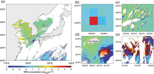
Speckles have been commonly appeared in optical images of the Geostationary Ocean Color Imager (GOCI) in the seas around Korea. GOCI, the first geostationary ocean colour satellite sensor, has observed the Northwest Pacific Ocean with an unprecedented high spatial resolution of 500 m ×$$500 m at one-hour interval (Figure 1(a)). Differently from other near-polar orbit ocean colour satellites such as SeaWiFS or MODIS, GOCI, using a push-broom scanning method, has frequently observed oceanic features every hour, approximately 8 times per day. It has produced SPM images including other oceanic variables such as chlorophyll-a concentration, water quality, and coloured dissolved organic matter (Figure 1(b)). Similar to previous ocean colour satellite images, numerous speckles are shown in GOCI images. One of the significant errors originates from the stray light effect of the GOCI sensor, which should be considered for a proper estimation of optical properties to enhance the data quality for further scientific analysis (Oh et al. 2011, 2013; Kim et al. 2015). The SPM is one of the ocean colour variables with higher possibility of speckle than any other parameters as inferred from general formula of the estimation of SPM, unlike chlorophyll-a concentration and CDOM.

Figure 1. (a) GOCI RGB image of the research area; the numbers in orange coloured boxes indicate observation order of the slots and (b) suspended particulate matter concentration (g m⁻³) image of the research area, where the white colours indicate clouds.

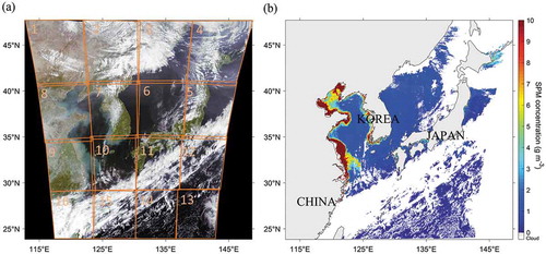
GOCI has observed the seas around Korea which consist of various types of water such as relatively clear water with SPM concentration of less than 0.00 g m⁻³–1.00 × 10⁻¹ g m⁻³ in the East Sea (the Japan Sea) (EJS) and the Northwest Pacific as well as highly turbid waters near very shallow estuaries and tidal mixing zones in the Yellow Sea (Figure 1(b)). In particular, highly turbid water with the highest concentration of SPM, up to 3.40 × 10² g m⁻³, appears in the shallow regions near the Yangtze River (Siswanto et al. 2011; Gao, Li, and Zhang 2012).

The objectives of this study are to 1) identify speckles apparent in GOCI images, 2) classify the speckles into several groups, 3) investigate the spatial and temporal variability of the speckles, 4) analyze the characteristics of the speckles, 5) understand the potential causes of each speckle group, 6) develop a methodology to eliminate the speckles as one of the quality control processes of SPM data, 7) estimate the capability of developing techniques for speckle removal by comparing composites filed before and after the quality control process, and 8) discuss the in-depth causes of the speckles in association with atmospheric correction.

2. Data and methods

2.1. Satellite data

GOCI is onboard the Communication, Ocean and Meteorological Satellite (COMS) and has observed the seas around the Korean Peninsula (24.75^°N – 47.25^°N, 113.40^°E – 146.60^°E) with a high spatial resolution of 500 m × 500 m and a high temporal sampling capability of 8 times per day from 9:00 AM (Ante Meridiem) to 4:00 PM (Post Meridiem) since June 2010. As shown in Figure 1(a), a whole GOCI image is obtained by combining 16 slots using a step-and-stare scanning method or a push-broom method (Kang et al. 2006; Faure, Coste, and Kang 2008; Kang et al. 2010). The scanning starts at the northwestern corner of the image, denoted as the number 1, and ends at the southwestern corner (the number 16) of the slots as shown in Figure 1(a). It has six visible (412 nm, 443 nm, 490 nm, 555 nm, 660 nm, and 680 nm) and two near-infrared (NIR) channels (745 nm and 865 nm) with a 20 nm bandwidth. Approximately six years of GOCI level 2 data of remote sensing reflectance (R_rs, measured in sr⁻¹) and SPM were collected from the Korea Ocean Satellite Center (KOSC) and utilized for this study.

2.2. Atmospheric correction

In this study, we used level 2 R_rs data radiometrically and geometrically corrected by the GOCI Data Processing System (GDPS) of KOSC. The atmospheric correction algorithm of the KOSC is composed of a series of procedures such as Rayleigh scattering, aerosol scattering, and genuine seawater reflectance (Gordon, Brown, and Evans 1988; Wang 2005; Gordon and Wang 1994a; Wang and Gordon 1994). The Rayleigh scattering is removed by considering diverse factors based on the channel wavelength, date, time, solar zenith angle, solar azimuth angle, satellite zenith angle, and satellite azimuth angle of each pixel (Gordon and Wang 1992; Wang 2002). If the Rayleigh corrected reflectance of 865 nm is greater than a threshold, the pixel is classified as cloud (Ahn et al. 2012).

To remove the aerosol scattering effect as a next step of the atmospheric correction, black pixel assumption, with no radiation from seawater in a NIR wavelength range such as 745 nm and 865 nm, was applied to the reflectance values (Wang and Gordon 1994). The up-to-date GOCI algorithm uses three types of aerosol models: a maritime aerosol model with 99.00% relative humidity (M99), a maritime aerosol model with 50.00% relative humidity (M50), and a coastal aerosol model with a relative humidity of 50.00% (C50) (Shettle and Fenn 1979). In the case of turbid water, an additional procedure is included by determining the relations between 660 nm, 745 nm, and 865 nm (Ruddick et al. 2006). Then, a vicarious calibration procedure is applied to the pixel by employing correlations between 660 nm and 745 nm and between 745 nm and 865 nm (Ahn et al. 2012). Abnormal radiances due to whitecaps from rough sea surfaces under strong windy condition are corrected by a wavelength-independent model based on the wind field and sea-surface temperature (Monahan 1971; Gordon and Wang 1994b). More detailed procedures on subsequent atmospheric corrections of GOCI are described in Ahn et al. (2012).

2.3. Calculation of suspended particulate matter

To estimate SPM from reflectance data, the GDPS suggests two types of SPM algorithms: the Yellow Sea Large Marine Ecosystem Ocean Color Work Group (YOC) algorithm and the Case II algorithm, based on three bands at 490 nm, 555 nm, and 660 nm (Siswanto et al. 2011; Min et al. 2012). In general, the total SPM concentration is determined gravimetrically in the laboratory with difference between tare weight (before filtration) and dry weight (after filtration) using a polycarbonate membrane filter or glass-fibre filter (GF/F) for sampled sea water (Strickland and Parsons 1972; Doerffer 2002). We selected the YOC algorithm, which has been reported to be more appropriate for the GOCI region based on in-situ water sampling and filtration (Siswanto et al. 2011). The fundamental formulation of GOCI SPM followed the previous research of Tassan (1994) using the ratio of the R_rs at 490 nm and 555 nm and the sum of the R_rs at the wavelengths of 660 nm and 555 nm of SeaWiFS in the Gulf of Naples. Coefficients of the YOC SPM in Equation (1) were empirically derived by using in-situ measurements in the GOCI region as follows:

(1) $\mathrm{S}\mathrm{P}\mathrm{M}={10}^{\left(0.649+25.623\left(R_{\mathrm{r}\mathrm{s}}\left(555\right)+R_{\mathrm{r}\mathrm{s}}\left(660\right)\right)-0.646\left(\frac{R_{\mathrm{r}\mathrm{s}}\left(490\right)}{R_{\mathrm{r}\mathrm{s}}\left(555\right)}\right)\right)}$(1)

Detailed validation results of the SPM retrievals are in Siswanto et al. (2011).

2.4. Detection method of speckles

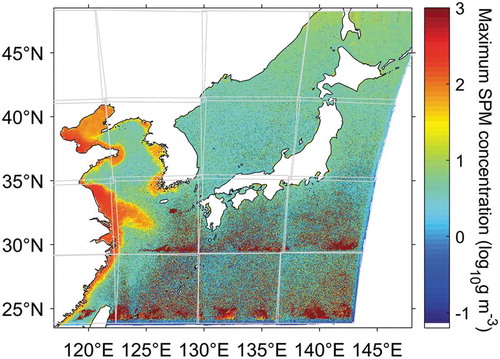
To identify the existence of SPM speckles, we tested if the maximum values of SPM at each pixel are distributed in a normal range of SPM in the GOCI region for 2015 (Figure 2). Previous literature has reported that the highest SPM concentration appeared at the entrance of the Yangtze River (Siswanto et al. 2011). The maximum SPM from the GOCI observation in 2015 also revealed similar values of up to 3.40 × 10² g m⁻³ in this location as shown in Figure 2. However, much higher values appeared, even in the majority of the Northwest Pacific region from 25.00^°N to 35.00^°N. Because this region is classified as clear water hundreds to thousands of kilometres from land, the unusual SPM values of this peculiar type can be regarded as speckles similar to the enormously high values of chlorophyll-a concentration speckles from satellite ocean color data of previous research studies (Chae and Park 2009; Park, Chae, and Park 2013). Pixels with erroneous speckles should be eliminated for diverse purposes of scientific research (e.g. Park et al. 2012, 2016).

Figure 2. Maximum suspended particulate matter concentration (log₁₀ g m⁻³) from GOCI data in 2015.

To remove the speckles from the level 2 hourly GOCI SPM image, we developed a sequential procedure for speckle detection based on the spatial and temporal characteristics of the speckle variations. Figure 3 illustrates the flowchart for speckle detection and the classification of speckle types. First, the monthly climatology of the speckle-free SPM was constructed for the standard reference data of SPM. As a first step, SPM values greater than 1.00 × 10³ g m⁻³ in each image were eliminated by considering the fact that the highest SPM concentration values are approximately 3.40 × 10² g m⁻³ near the Yangtze estuary (Siswanto et al. 2011; Gao, Li, and Zhang 2012). Then, a recursive procedure to reject the speckles was conducted by taking a median value several times for a given month. The final median value at each pixel location during one month was selected as a representative SPM of monthly climatology. Through this procedure, we could exclude the inclusion of abnormally high values induced by speckles as well as erroneous low values induced by the effect of cloud shadow on the estimation of SPM.

Figure 3. Flowchart of the speckle detection and classification process for GOCI SPM data (MCSPM: Monthly climatology SPM, STD9: 3 × 3 window standard deviation (STD), Mean9: 3 × 3 window mean, STD8: STD except centre in 3 × 3 window, Mean8: mean except centre in 3 × 3 window).

A series of speckle detection procedures was applied to every SPM value in each pixel of the GOCI image as shown in the upper part of Figure 3. First, if SPM values, identified as non-cloud values, exceeding 1.00 × 10³ g m⁻³, they were classified into speckles. Each threshold was determined through extensive empirical scrutiny of the speckle values. Second, considering speckles with relatively small SPM values are clear water, such as the EJS, a pixel satisfying the limits (Threshold, T) of low SPM from the monthly climatology (< T₁ (1.00 × 10⁻¹ g m⁻³)) and high SPM (> T₂ (2.00 g m⁻³)) at the same position was regarded as a speckle. Occasionally, the speckle appears not as a congregated one but as an isolated one, which is clearly evident from its neighbouring normal values. A speckle of this type was adaptively identified by the difference (> T₃ (0.1)) between the ratio of the standard deviation to a mean value of all values within a 3 × 3 window and that of the eight values except the SPM at the centre of the window. The SPM values of cloud-induced speckles are several times greater than the climatology data near the clouds (distance <5 km) over the clear ocean. The threshold of the cloud peripheral region is determined based on a correlation between the SPM value of the speckle and the distance from the cloud. The pixels contaminated due to clouds were removed by providing upper (> T₄ (2) times the SPM from climatology) and lower limits (< T₅ (0.5) the SPM from climatology) of SPM near clouds (<5 km). These speckles were classified into four types based on physical properties and potential causes as described specifically in the next section.

3. Results

3.1. Probability of speckle appearance

In order to investigate how frequently speckles appear in a given pixel in the entire study region, we estimated the probability P (%) of speckle appearance as Equation (2):

(2) $P\left(\mathrm{\%}\right)=\frac{n}{N}100$(2)

where n is the number of speckles and N is the number of observed SPM at a given pixel after the cloud-masking procedure. The monthly distribution of the maximum probability in Figure 4 shows 30.00% on the whole, but a high probability of up to 50.00% appeared particularly in December. First, the probability of the EJS shows dominant seasonality with a relatively high probability of approximately 30.00% during winter (from December to February) and the lowest probability of less than 5.00% during spring (April to May). During summer, the probability tended to weakly increase until August and then decrease in September. One of the interesting features is the obvious contrast between the continental and offshore sides of the EJS. The continental side reveals no conspicuous speckles with a low probability (<5.00%). In contrast to this, the off-shore side near the Japanese coast had extremely high probability (>25.00%). This specific pattern is quite similar to the cloud distribution, with cumulus clouds over the EJS during winter as mentioned by Chae and Park (2009) and Park, Chae, and Park (2013).

Figure 4. Monthly spatial distribution of speckles during 2015. Colours indicate percentage of speckle appearances when the SPM concentration data were obtained. (a) January, (b) February, (c) March, (d) April, (e) May, (f) June, (g) July, (h) August, (i) September, (j) October, (k) November, and (l) December.

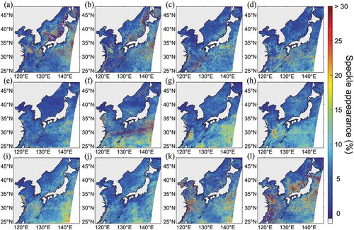
High probability of this type, induced by an array of small cumulative clouds, also appeared in the northeastern part of the Northwest Pacific during winter. However, during summer, the local maximum (>30.00%) of the speckle probability of the Northwest Pacific appeared south of Japan along latitude 30.00^°N as clearly shown in the map of June (Figure 4). The Yellow Sea has a random distribution of probability of less than 15.00%. On the other hand, a more than 20.00% value appeared in near the Yangtze River and the Bohai Sea during November and December. One of the important lessons learned from the monthly speckle probability map is that the speckle probability itself has seasonality, but appeared everywhere in the study region regardless of specific places.

3.2. Speckle types

Figure 5(a) shows an example of an SPM concentration image containing numerous speckles at 4:00 Universal Time Coordinated (UTC) on 3 June 2015. Overall, the SPM varied from 1.00 × 10⁻² g m⁻³ to more than 1.00 × 10³ g m⁻³. However, the enlarged images, marked in red boxes, revealed abnormally high SPM values of greater than 1.00 × 10³ g m⁻³ as shown in Figure 5(b–e). These speckles presented specific characteristics in terms of their spatial distributions. Some appeared as a single pixel, while others appeared as a congregated patch or an array-like feature. Thus, we classified all the speckles into several groups as follows.

Figure 5. (a) GOCI SPM concentration (log₁₀ g m⁻³) image of the research area, with examples of (b) isolated speckle referred to area 1, (c) cloud edge speckles referred to area 2, (d) patch shape speckles referred to area 3, and (e) slot-related speckles referred to area 4 in subfigure (a) at 4:00 UTC on 3 June 2015.

3.2.1. Isolated speckle

As shown in Figure 5(b), in the zoomed region of the box (b) of Figure 5(a), only a single pixel presented a high SPM concentration (9.48  × 10³ g m⁻³), which is extremely high as compared to the SPM values (1.00 × 10⁻² g m⁻³–1.00 × 10⁻¹ g m⁻³) of its neighboring pixels. The value is 9.24 × 10⁴–7.03 × 10⁵ times larger than the surrounding values, which is a very unusual feature. This speckle tended to appear as a single point and as an isolated point in clear contrast to the adjacent pixels. Previous literature termed this speckle as ‘pixelization’ referring to one or two spatially discontinuous pixels with anomalous values over the ocean (Hu, Carder, and Muller-Karger 2000; Robinson et al. 2000; Hooker et al. 2003).

3.2.2. Near-cloud speckle

Some of speckles in Figure 5(a) appeared as a band-like or array-like feature around many scattered clouds. Figure 5(c), an enlarged portion of (c) in Figure 5(a), exhibits three different ranges of SPM concentrations of the speckles such as enormously high values (>1.00 × 10³ g m⁻³) (red color), medium-range values (3.00 g m⁻³–1.00 × 10² g m⁻³) (yellow color), and under-speckles with extremely low values (as denoted in blue color).

Extremely high values are randomly distributed near the clouds (Figure 5(c)). However, the medium-range speckles, marked in yellow colour, tended to appear mostly in the western part of the clouds. Their SPM values are estimated to be much higher than normal SPM values, which cannot be seen in the EJS. This might be related to a moisture effect due to the eastward movement of the clouds, which will be discussed in the later section. Previous studies have also shown that speckles increase at the edge of scattered clouds (Robinson et al. 2000; Hooker et al. 2003; IOCCG 2004; Chae and Park 2009; Park, Chae, and Park 2013). In contrast, the under-speckles with the lowest SPM tended to appear on the eastern side of the clouds. This is related to the effect of the cloud shadow being opposite to the position of the sun.

3.2.3. Patch-type speckle

Unlike previous speckle types in Figure 5(b,c), some speckles congregate and occupy a wide area of 0.5° × 0.7° as shown in the southern region of Jeju Island (Figure 5(c)). The SPM values are extremely elevated from at least 1.00 × 10³ g m⁻³ to order of 37 (O (37)) g m⁻³ as compared to the neighbouring pixels with normal ranges of approximately 1.00 × 10⁻² g m⁻³–2.00 g m⁻³. The spatial distribution of the speckles appears in a patch shape (termed a ‘patch-type speckle’ hereafter), which is quite dissimilar to the isolated or narrowly elongated shape in Figure 5(b,c). In contrast, one of the similar features of this type to Figure 5(c) is that the high-value speckles are accompanied by under-speckles with abnormally low values (<1.00 × 10⁻⁴ g m⁻³) around them (Figure 5(d)). These features appeared in places with relatively high humidity after the passage of eastward-moving clouds. This might be induced by the effect of water vapour in the atmospheric correction. Details on this conjecture and potential causes will be presented in the following sections.

3.2.4. Slot-related speckle

A very high SPM concentration occurs at the southeastern part (e) of Figure 5(a) in the Northwest Pacific. This area usually has small SPM values of 1.00 × 10⁻² g m⁻³–1.00 g m⁻³, because it is more than 600 km from land. Thus, these pixels with high SPM values (1.00 × 10² g m⁻³–1.00 × 10³⁵ g m⁻³) at the northern part of Figure 5(e), coloured in red, seem not to be natural but can be regarded as speckles. One of the distinct features of this type is the existence of a dominant interface, divided by a zonal line, between the abnormally high SPM in the northern region and the low SPM in the southern region. This north-south boundary coincides with the interface between the 12^th and 13^th slots of GOCI as denoted in Figures 1 and 2. Extremely high SPM values occurred at the lower portion of the 12th slot. This is inferred to be related to the effect of instrumental correction problem such as the previously reported stray light issues induced by inner slot response (Oh et al. 2011, 2013; Kim et al. 2015), which will be discussed in later section. Thus, we termed this type of speckle a ‘slot-related speckle.’

3.3. Spatial distribution of speckles

In order to understand how frequently each speckle appeared at a given pixel, we identified and classified the speckles into five classes by applying a scheme suggested in the lower diagrams of Figure 3. First, a single speckle, only a speckle within a 3 ×$$3 frame and 5 km from clouds, was treated as the ‘isolated speckle’. The ‘patch-type speckle’ was detected by applying criteria with greater areal extent by occupying over T₆ (80.00%) of a 70 km × 70 km window. The speckle located at a short distance within 5 km from the boundary of clouds is considered to be a ‘near-cloud speckle.’ It includes speckles induced by cloud shadowing, which can be discriminated by having an n-times lower value compared to the monthly climatology SPM value. Other remaining speckles, not classified into any of these speckle types, are determined to be ‘slot-related’ speckles.

Figure 6(a) shows the spatial distribution of all speckles containing all types using 2920 (8 times multiplied by 365 days) GOCI images during 2015. Because of unequal cloud cover from different passage of clouds, the number of GOCI observations without a cloud is not the same but varies for every pixel. Under such differential cloud coverage, most speckles are apparently visible in the southeastern part of the GOCI region (Figure 6(a)). The maximum number of speckles reached up to 120 times in one year during 2015. In the case of isolated speckles, they are distributed throughout the entire region with similar frequencies as shown in Figure 6(b). We calculated how many times the isolated speckles appear at a given pixel for one year. As a result, the speckles of this type were thought to be randomly distributed with relatively high uniformity. Speckles with an appearance frequency more than once were rarely seen, less than 1.00% of the total. Those with a frequency of two times over a year were very small in number, 977 pixels out of 88,717 pixels. This implies that there would be a certain mechanism to generate this sort of randomness.

Figure 6. Frequency map of speckle distribution based on each speckle type in 2015. Colour represents the number of each type of speckles; (a) all (b) isolated, red box indicates enlarged image, (c) near-cloud with high SPM, (d) induced by cloud shadowing, (e) patch type, and (f) slot-related.

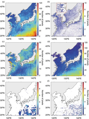
Near-cloud speckles shown in Figure 6(c) have a somewhat high frequency ranging from 10 to 50 times for each pixel per year. They tended to be high in the coastal regions near land such as the continental side of Korea and China, and along the southwestern coast of Japan. In addition to this distribution, the Northwest Pacific far from coastal areas also has relatively high numbers of greater than 30. Under-speckles with abnormally low SPM values, related to cloud shadows or water vapour, had low frequencies (<20) in the EJS and the East China Sea, which was in contrast to high frequencies (>100) in the Northwest Pacific (Figure 6(d)).

The patch-type speckles had an area ranging from 60 km² to 30,000 km² and were particularly concentrated at the southeastern part of the research area (Figure 6(e)). The maximum frequency of this type reached up to four times at a given pixel for one year during 2015. Except for the three types of speckles previously described, there was a significant number of residual speckles unidentified to any types as shown in Figure 6(f) (all speckles (Figure 5(a)) minus the sum of speckles (Figure 5(b–e)). This type of speckle tended to be mostly distributed along the lower part of the slots, particularly at slot numbers 10–15, in the Northwest Pacific. However, slot-related speckles were found even within the spatial distribution of other speckle types, for example, as shown in the manifest boundary along a zonal line of 29.00°N in Figure 6(d).

3.4. Causes of speckles

3.4.1. Isolated speckle

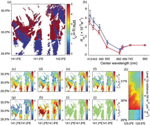
Although SPM values of isolated speckles are extremely high as shown in Figure 7(a), R_rs values at each band of the speckle are not that high, but rather small as compared to those of speckle-free pixel values (Figure 7(a,b)). Even the overall pattern of R_rs of a speckle is quite similar to a speckle-free pixel with respect to a wavelength from 412 nm to 865 nm. The only difference is found in the sign of R_rs values, especially at wavelength of 555 nm. The spectral characteristics (Figure 7(b)) indicate that the ratio of the small negative R_rs(555) and the large positive R_rs(490) can increase the SPM concentration to extremely high value due to the ratio of R_rs(490) to R_rs(555) in the SPM Equation (1) and its negative sign.

Figure 7. (a) SPM concentration (g m⁻³) of an isolated speckle, (b) level 2 spectral remote sensing reflectance (sr⁻¹) of the isolated speckle (red) and speckle-free (blue) and spatial remote sensing reflectance of the (c) 412 nm, (d) 443 nm, (e) 490 nm, (f) 555 nm, (g) 660 nm, (h) 680 nm, (i) 745 nm, and (j) 865 nm centered wavelength channels.

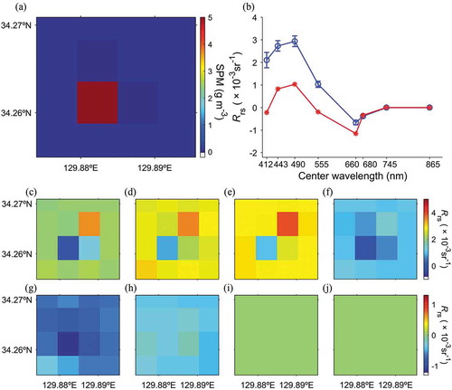
The spatial distribution of R_rs of each channel is shown in Figure 7(c–j). At the location of the isolated speckle, the R_rs values of the visible channels are lower than those of neighbouring pixels. This weakly negative value at 555 nm is expected to provide an abnormally high SPM value. In general, sub-pixel clouds may produce a somewhat high reflectance as shown in Figure 7(c–e). Considering that a cloud has a high R_rs in all visible channels (Frey et al. 2008), an isolated speckle is supposed to be generated by an unmasked small cloud fraction smaller than one pixel and a small fast-moving cloud. GOCI adopted a push-broom manner within each slot and has used a specific order (660 nm – 555 nm – 745 nm – 443 nm – 680 nm – 412 nm – 865 nm – 490 nm channels) in its observation of the sea (Ahn et al. 2012). GOCI uses an iterative scheme of the ratio between the 745 nm and 865 nm channels for atmospheric correction. The spatial distribution of the reflectance of each band (not shown here) reveals that the maximum reflectance of 745 nm and 865 nm are located at different positions, the left lower and right upper parts of the image in Figure 7(c–j), respectively. This differential spatial distribution can produce extremely high speckle numbers due to a failure of the atmospheric correction procedure. It is supposed to be induced by cloud movement during the time gap (60 s) between the 745 nm and 865 nm channels used for the atmospheric correction. If the cloud moves faster than 8.3 m s⁻¹ (500 m per 60 s), the ratio of the two channels is disturbed by undetected cloud radiance, causing an error in the estimation of the atmospheric correction. It is common that the wind speed is faster than 8.3 m s⁻¹ over the ocean, and thus speckles induced by cloud movement occur all the time.

3.4.2. Speckles near clouds

As shown in Figure 5(c), there are three different types of speckles near clouds over a very calm region (<2.00 g m⁻³) of the EJS, including enormously high SPM values greater than 1.00 × 10³ g m⁻³; an intermediate range of 3.00 g m⁻³–1.00 × 10² g m⁻³, which can be observed in the turbid coastal water but not in the clear water (Figure 1(b)), and reverse speckles with non-negative and extremely low values less than 1/1000 of the climatology data. We classified the pixels in Figure 5(c) into four classes: the three types of speckles (extremely high speckle, relatively high speckle, extremely low speckle) and speckle-free normal pixels. Spectral characteristics of the four classes in Figure 8(a) reveal that the high speckles (marked in red) have similar tendency with the spectral distribution of R_rs of the previous isolated speckles (the red line in Figure 7(b)) except a different sign of R_rs at 412 nm and 680 nm, which are not included in SPM algorithm.

Figure 8. (a) Spectral remote sensing reflectance (sr⁻¹) of cloud edge speckle (extremely high, relatively high, extremely low in red, green, black, respectively) and speckle-free (blue), (b) two-dimensional histogram at each bin of SPM concentration (log₁₀ g m⁻³) of speckle in relation to distance from cloud (km), (c) spectral remote sensing reflectance (sr⁻¹) of a patch-shape speckle (red) and speckle-free (blue), (d) temporal cloud movement from 1:00 UTC to 5:00 UTC during the same day.

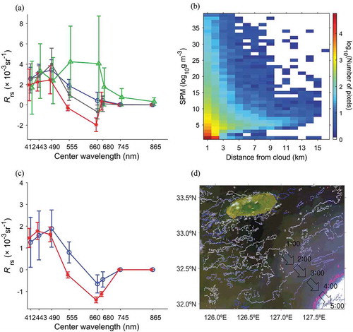
In the case of the relatively high SPM values (green line in Figure 8(a)), their spectral characteristics are quite similar to that of turbid water having a relatively high peak R_rs at 555 nm (Robinson 2004). Because the study region is regarded as having very clear water without high turbidity, the high R_rs(555) and R_rs(660) values seem unusual, which finally results in a higher SPM value due to the contribution of the sum between the two channels (555 nm and 660 nm) as shown in Equation (1). This locally uncommon spectral pattern is probably produced by spectral contamination from very thin clouds or cloud movement within a few pixels.

The cloud masking of GOCI is based on the R_rs of the 412 nm and 865 nm channels, the 6^th and 7^th order of GOCI observations within a slot. By contrast, SPM is calculated mainly by the 1^st and 2^nd order of GOCI observations (555 nm and 660 nm). This implies the possibility of a failure in the cloud-masking procedure because of a high temporal difference between the channels for cloud masking (412 nm and 865 nm) and the two main channels (555 nm and 660 nm) for SPM calculation. The time differences between the channels amount to 60–90 s at a maximum. Thus, it is inferred that the effect of the time difference may be significant in the estimation of SPM when the wind blows faster than 5.5 m s⁻¹ (500 m divided by 90 s). The other speckles with extremely low SPM are probably a result of a cloud shadow. The low reflectance at 555 nm and 660 nm (grey line in Figure 8(a)) contribute to the abnormally low SPM as shown in the first two terms in Equation (1).

In order to understand how frequently the under- and over-speckles appear near clouds, we calculated a histogram of the frequency number of speckles as a function of SPM concentration and distance from the clouds using all of the GOCI images during 2015 (Figure 8(b)). The majority of speckles were found a short distance of less than 5 km from a cloud edge. The speckles tended to be greatly reduced or nonexistent at long distances (>15 km) from cloud edges.

3.4.3. Patch-type speckles

Figure 8(c) shows the spectral distribution of R_rs values for speckle-free pixels (blue) and patch-type speckles (red) as shown in Figure 5(d). A difference in the two spectral distributions can be seen from the opposite signs of R_rs(555) that is one of the most important factors in SPM estimation. The other difference from the extremely high speckles in Figure 8(a) is the opposite signs of R_rs at 680 nm. Although R_rs(680) is not one of the controlling factors of speckles as inferred from Equation (1), the unusual negative values provide a hint regarding poor atmospheric correction, especially water vapour correction.

In order to investigate if the patch-type speckles are related to clouds or water vapour concentration in the air, we examined the existence of clouds near the patch-type speckles. Figure 8(d) shows the contours of cloud edges (marked in white lines) from 1:00 UTC to 5:00 UTC on the same date with the patch-type speckles over a Red Green Blue (RGB) image at 4:00 UTC. The cloud moved from the northwest to the southeast for the four hours. The RGB image reveals the thick cloud at the right corner (denoted in the magenta colour) and to the left atmospheric water vapour behind as shown in bright white in Figure 8(d). It is difficult to remove the effect of water vapour using only GOCI channels, which requires additional bands at 6.72 μm, 8.55 μm, and 12.0 μm to discriminate high-, mid-, and low-moisture conditions (Ackerman et al. 1998). Thus, the water vapour is inferred to contribute to the negative R_rs values at 555 nm, 660 nm, and 680 nm during the atmospheric correction procedure and then generate speckles with extremely high SPM values behind the horizontal movement of clouds.

3.4.4. Slot-related speckles

Figure 9(a) is the linear scale of Figure 5(e), and again the distribution of the values at the boundary between the two slots is significantly different. The characteristics of the speckle area on the 12^th slot and the speckle-free area on the 13^th slot are shown as red and blue lines in Figure 9(b). Similar to other types of speckles, it has negative reflectance at 555 nm, 660 nm, and 680 nm. However, it shows relatively high reflectance at 412 nm and 443 nm, similar to that of the clear ocean. Why are there negative values at 555 nm, different from the surrounding values? The cause of this seems to lie in the atmospheric correction process. It is assumed that the R_rs value of 680 nm, which is the standard of atmospheric correction, may have caused the problem.

Figure 9. (a) SPM concentration (g m⁻³) with speckle near the slot edge, (b) spectral remote sensing reflectance (sr⁻¹) of enormously high SPM value at the speckle (red) and normal ocean (blue) and the spatial remote sensing reflectance (sr⁻¹) of the (c) 412 nm, (d) 443 nm, (e) 490 nm, (f) 555 nm, (g) 660 nm, (h) 680 nm, (i) 745 nm, (j) 865 nm centered wavelength channels; (k) level 1b radiances (W m⁻² μm⁻¹ sr⁻¹) of the 865 nm channels.

Figure 9(c–j) illustrate the decreasing tendency toward the lower part of the slot in most of the channels, except for 680 nm, which is due to the fact that the atmospheric correction of aerosol scattering is based on the reflectance at 680 nm. Because of the abnormally high reflectance at 680 nm, reflectance of the visible channels has overcorrected the aerosol scattering data in the lower part of the slot. It has been reported that the radiance detected in the lower part of the slot shows a higher value due to the stray light generated by internal circumstances in the sensor (Kim et al. 2015).

Previous near-polar orbit ocean colour sensors scan horizontally or vertically with respect to the direction of the movement of the sensor: whisk broom (SeaWiFS, MODIS) or push broom (Medium Resolution Imaging Spectrometer). Unlike these sensors, GOCI as a sensor of a geostationary satellite adopts a ‘step and stare’ mode that observes each channel in a slot sequentially and then moves to a neighboring slot continuously until the last slot (Figure 1(a)) (Kang et al. 2006; Faure, Coste, and Kang 2008; Kang et al. 2010). The stray light effect, as one of the mechanical problems of GOCI, may contaminate original signals from the sea surface by inflating the signals at the lower part of the slot (Oh et al. 2011, 2013; Kim et al. 2015). There are large differences in observation times between slots. These differences generate much larger differences at the slot boundary between the north-south slots compared to the east-west slots because of time gaps. As a result, spatial distributions of SPM tend to have obvious meridional contrast at the boundary following the bottom of each slot as shown in Figure 9(a).

Level 1b radiance data at 865 nm as shown in Figure 9(k) exhibits this type of slot effect. Because of this unnecessary and contaminated noise, the reflectance values of each band are possibly abnormal even after atmospheric correction. During the atmospheric correction process, a black pixel assumption is applied to eliminate aerosol scattering by assuming that the NIR is nearly zero under a clear water condition. According to GOCI atmospheric correction (Ahn et al. 2012), the reflection of aerosol is calculated based on 745 nm and 865 nm. However, the values at 745 nm and 865 nm, which are abnormally high at the bottom of the slot due to the stray light effect (Figure 9(k)), are likely to underestimate R_rs(555) to be a weakly negative value. Nearly-zero values of the two bands in Figure 9(i,j) imply the subtraction of the aerosol effect in the reflectance at the NIR bands. As previously mentioned, the negative sign of R_rs(555) is responsible for the extremely high speckles. The effects of combined factors such as stray light and time differences can generate a large number of speckles near the bottom of each slot as clearly shown in the southern region of Figure 2.

3.5. Results of speckle removal

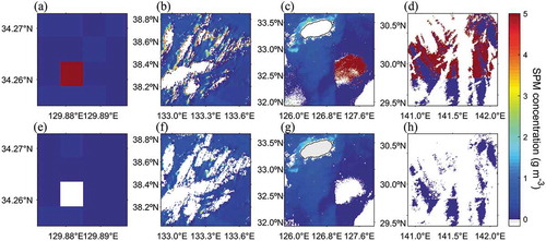
In order to remove the speckles, we identified speckles and classified them into five classes as shown in the lower part of Figure 3. Figure 10 shows the speckle removal results for each type of speckle applying our algorithm. An isolated speckle of approximately 1.00 × 10⁵ g m⁻³ was extracted from the adjacent normal values of approximately 7.00 × 10⁻² g m⁻³ (Figure 10(a,e)). In the case of near-cloud speckles (Figure 10(b)), 6.22% of the speckles of the subsampled region were eliminated (Figure 10(f)). As a result, the extraordinarily high values of approximately 1.42 × 10³³ g m⁻³ were adequately removed as shown in Figure 10(f). Through the removal procedure, patch-type speckles (mean value: 3.18 × 10³⁴ g m⁻³) occupying 5.85% of the second subsampling area as well as the slot-related speckles were all removed (Figure 10(g,h)). After removing the slot-related speckles, the mean value was decreased dramatically from 1.87 × 10³⁵ g m⁻³ to a more typical SPM concentration of approximately 1.00 × 10⁻² g m⁻³.

Figure 10. Examples of four types of speckles; (a) isolated, (b) near-cloud, (c) patch-type, (d) slot-related, as a result of the speckle removal, (e) from (a), (f) from (b), (g) from (c), and (h) from (d), respectively. Colors indicates concentration of particulate matter.

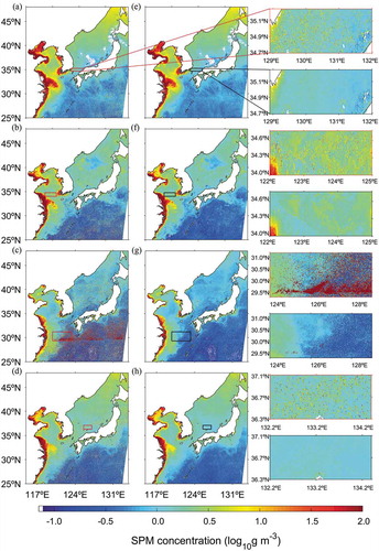
To investigate the impact of the speckles on monthly variations in SPM, we estimated the spatial distribution of the monthly maximum of SPM for representative seasonal months (January, April, July, and October) in 2015 before and after the speckle-removal procedure (Figure 11). In the case of the EJS, the salt-and-pepper-coloured features in the red boxes in Figure 11(a,d) completely disappeared after the speckle-removal procedure (Figure 11(e,h)). Similar speckles with a stripe pattern in the Yellow Sea during April (Figure 11(b)) were also clearly removed as shown in the enlarged portion of Figure 11(f). The maximum SPM image during July (Figure 11(c)), after the procedure, also revealed noise-free features free from highly concentrated slot-related speckles induced by the stray light effect at the lower part of the 10^th–12^th slots (Figure 11(g)). The congregated speckles related to the slots prevented examination of the spatial distributions of SPM in the East China Sea and a part of the Northwest Pacific south of Japan. The removal procedure manifestly revealed the spatial structure of SPM in these areas as shown in the zoomed portion. A result of this type implies the significance of the erroneous-speckle-removal procedure in the diverse applications of SPM to study spatial and temporal variability of SPM.

Figure 11. Monthly composite images of raw SPM data during (a) January, (b) April, (c) July, (d) October, and their extensions (red box), and reprocessed monthly composite image during (e) January, (f) April, (g) July, (h) October, and their extensions (black box).

3.6. Reduction of six-year speckle-induced errors

To clarify the effect of the speckle removal, we reprocessed the level 2 SPM data from April 2011 to November 2016 and compared the difference between the SPM data before and after the removal process (Figure 12). Figure 12(a) indicates dominant seasonal variations of SPM values with extremely high SPM values (>O(30) g m⁻³) during the summer from June to July and very small values (<1.00 g m⁻³) during the winter. A tendency of this type is completely opposite to the previous knowledge, where the SPM values show a maximum during winter and a minimum during summer with the range of 0.00 g m⁻³–5.00 g m⁻³ (Yanagi et al. 1996; Yuan et al. 2008; Bi et al. 2011; Son et al. 2014). The month-year plot of the reprocessed data after undergoing the removal procedure reveals a completely reversed trend in the seasonal variation of the SPM values in this region (Figure 12(b)), which coincides well with the commonly known results, with high values due to strong northerly or northwesterly winds during the winter (Yanagi et al. 1996; Yuan et al. 2008; Bi et al. 2011; Son et al. 2014). This significant difference between Figure 12(a,b) suggests that GOCI speckles are predominantly affecting the SPM values during the summer. The histograms of the speckle-containing SPM data and reprocessed SPM data (Figure 12(e,f)) also support the importance of the speckle removal process developed in this study. Abnormal peaks disappear during the summer and normal seasonal distribution with a maximum peak during winter is adequately presented.

Figure 12. Month-year plot of SPM concentration from (a) GOCI level 2 data and (b) reprocessed data after the speckle-removal process for the period from 2011 to 2016, the monthly variations of the six-year average SPM for (c) the SPM data of (a) and (d) reprocessed SPM values after the removal process, and the histograms of SPM (e) before and (f) after the process.

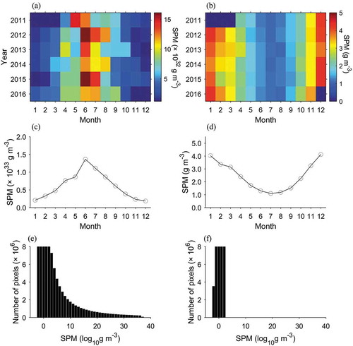
The number of the eliminated speckles was approximately 6.06% of the total number of observed pixels. However, the speckle pixels have a significant influence on the spatio-temporal variability of the SPM data, enough to change the overall temporal variability as illustrated in Figure 12. Therefore, it is expected that such erroneous speckles should be necessarily removed through the removal process prior to analysis.

4. Discussion

Through in-depth analyses of the spatial and temporal variability of erroneous SPM values, we were able to attempt to understand the potential causes of the speckles within the GOCI data. As a representative study of the speckles of ocean colour variables, Hu, Carder, and Muller-Karger (2000) clarified that SeaWiFS data reduced 35.00% of the speckles of chlorophyll-a concentration by improving atmospheric correction. Most GOCI speckles are expected to be associated with a partial failure in atmospheric correction, especially in a region under the atmospheric conditions of high humidity or a high number of aerosols. If the atmospheric correction of the GOCI data is improved, both the patch-type and some of the speckles near clouds could be essentially eliminated. GOCI does not contain a near-infrared channel that can observe the amount of water vapour or discriminate thin cirrus. Water vapour data from National Centers for Environmental Prediction with 2.5° × 2.5°, freely available in near real time, are too coarse to be utilized for high-resolution (up to 500 m) data using the atmospheric correction procedure for GOCI (GOCI Data Processing System version 1.3). When local phenomena occur, error from atmospheric correction is generated. If the quality of the atmospheric correction of the present GOCI algorithm were improved in the near future, the majority of the speckles could be effectively reduced.

GOCI has adopted a step and stare scanning method which is quite different from other ocean colour sensors such as SeaWiFS, MODIS, ENVISAT, or Nimbus-7. While a sensor observes the ocean surface within a slot using the scanning method, clouds can move over hundreds of meters during the time interval between the observations of each channel of GOCI. In particular, if the time interval between the channels used for cloud detection is relatively long, it can create speckles such as those previously mentioned. These types of errors are unavoidable mechanically; thus, the speckle pixels should be necessarily removed through the improved algorithm of speckle detection. Thus, the cloud detection algorithm of GOCI needs to be reinforced for this improvement. Other method based on the false spectral shape is likely to fail in the detection of speckles with moderate values in the non-turbid waters. In light of this, the present method can be applied both highly turbid waters and non-turbid clear water.

It has been commonly mentioned that an accurate modelling of instrumental stray light, as an additional part of an imaging system, has to be necessarily considered in the level of level 1b status to increase the number of useful pixels (IOCCG 2012a). Although a post-launch vicarious calibration removes a global bias from the data, it is difficult to eliminate the scene-specific errors completely (e.g. effects of instrumental polarization sensitivity, stray light, etc.) (IOCCG 2012b). GOCI also has essential instrumental problems related to the slot. In addition to the sharp disconnections between neighbouring slots, there is another issue related to the response phase in the inner slot termed the stray light effect (Oh et al. 2011, 2013; Kim et al. 2015). These characteristic effects become increasingly intensified at the bottom of each individual slot. This tendency becomes even greater when the atmosphere is humid. A method to fix the effect of the slot boundary was suggested by multiplying the inverse phase function of the slot response along the slot boundary (Kim et al. 2015). It is anticipated that the method would reduce the slot-related speckle, but it is still completely applicable to all the cases of speckles.

5. Summary and conclusion

This study provides a comprehensive understanding of GOCI SPM speckles, which will lead to better use of scientific applications, based on an in-depth investigation of spatial and temporal speckle variability as well as their causes. The major findings of this study are summarized below according to objectives 1–8 outlined in the ‘Introduction’ of this study:

1) Over one year, the spatial distribution of the maximum values of GOCI-derived SPM concentrations at each pixel showed irregular and randomly scattered speckles with very high SPM concentrations (exceeding 1.00 × 10³ g m⁻³).

2) The SPM speckles could be classified into several groups as follows: a single speckle isolated from its neighbouring normal pixels; patch-shape speckles; cloud-edge-related speckles, including a cloud shadow effect; and speckles related to a stray-light effect. The development of a sequential procedure for the detection and classification of SPM speckles demonstrated that the speckles were sufficiently eliminated to enable investigation of the spatial and temporal characteristics of SPM variations over long periods of time.

3) Analysis of the spatial and temporal variability of SPM speckles showed that they frequently occurred in the northwest Pacific, and were especially concentrated near the southern part of each slot boundary.

4) The occurrence of speckles showed seasonal and local characteristics in terms of apparent frequency and appearance probability. The monthly distribution of the maximum probability at a given pixel amounted to 0.3 on the whole, but the highest probability reached 0.5, and was particularly common in December.

5) Investigation of the potential causes for each speckle group revealed that an isolated speckle was caused by the movement of clouds during a temporal gap between observations in the 745 and 865 nm channels used for atmospheric correction. This study suggested that there is a certain limit of wind speed or cloud movement speed (>8.3 m s⁻¹) beyond which the possibility of SPM speckle generation becomes high; this is because of the time difference between the channels. In addition, the mechanisms of all types of speckles, including the patch-type and slot-related ones, were presented.

6) A methodology to eliminate speckles was developed as part of the quality control processes for SPM data, based on a statistical distribution of speckle values. The procedure suggested that the erroneous-speckle removal procedure was significant, among the diverse applications of SPM, for the study of spatial and temporal SPM variability.

7) The speckle removal abilities of the developed techniques were clearly apparent from a comparison of the composites filed before and after the quality control process. The eliminated speckles had occupied about 6.06% of the total number of observed pixels. However, the speckled pixels had a significant influence on the spatial and temporal variability of the SPM data, and were able to modify the overall temporal variability. Therefore, it is necessary to remove erroneous speckles prior to analysis.

8) This paper discussed the causes of speckle and all aspects of GOCI observations, including slot-related and atmospheric correction issues, in detail.

The problems related to speckles are expected to be significantly reduced by improving the atmospheric correction procedure and reducing noises, as well as by further advancements in the processing of GOCI data in the future. However, even if the version of the GOCI database is upgraded based on the upcoming algorithm in the near future, these types of speckles are likely to occur randomly and consistently. Therefore, it is crucial for level 2 users to reduce the errors by reprocessing the level 2 ocean colour data prior to diverse scientific research. Otherwise, the anomalously high SPM values would prevent users from properly understanding natural oceanic phenomena. Thus, this study addresses the decisive importance of speckle issues and recommends one means to further exclude GOCI SPM speckles of level 2 data based on their regional spatiotemporal characteristics.

Acknowledgments

This research was a part of the project titled ‘Development of the integrated data processing system for GOCI-II’ [grant number 1525007470] funded by the Ministry of Oceans and Fisheries (MOF), Korea. This study was partly supported by the project titled ‘Long-term change of structure and function in marine ecosystems of Korea’ [grant number 1525007947] funded by the Ministry of Oceans and Fisheries, Korea.

Disclosure statement

No potential conflict of interest was reported by the authors.

References

- Ackerman, S. A., K. I. Strabala, W. P. Menzel, R. A. Frey, C. C. Moeller, and L. E. Gumley. 1998. “Discriminating Clear Sky from Clouds with MODIS.” Journal of Geophysical Research: Atmospheres 103 (D24): 32141–32157. doi:10.1029/1998JD200032.
- Ahn, J. H., Y. J. Park, J. H. Ryu, B. Lee, and I. S. Oh. 2012. “Development of Atmospheric Correction Algorithm for Geostationary Ocean Color Imager (GOCI).” Ocean Science Journal 47 (3): 247–259. doi:10.1007/s12601-012-0026-2.
- Ahn, Y. H., J. E. Moon, and S. Gallegos. 2001. “Development of Suspended Particulate Matter Algorithms for Ocean Color Remote Sensing.” Korean Journal of Remote Sensing 17 (4): 285–295.
- Barnes, R. A., R. E. Eplee, G. M. Schmidt, F. S. Patt, and C. R. McClain. 2001. “Calibration of SeaWiFS. I. Direct Techniques.” Applied Optics 40 (36): 6682–6700.
- Bi, N., Z. Yang, H. Wang, D. Fan, X. Sun, and K. Lei. 2011. “Seasonal Variation of Suspended-Sediment Transport through the Southern Bohai Strait.” Estuarine, Coastal and Shelf Science 93 (3): 239–247. doi:10.1016/j.ecss.2011.03.007.
- Binding, C., D. Bowers, and E. Mitchelson-Jacob. 2003. “An Algorithm for the Retrieval of Suspended Sediment Concentrations in the Irish Sea from SeaWiFS Ocean Colour Satellite Imagery.” International Journal of Remote Sensing 24 (19): 3791–3806. doi:10.1080/0143116021000024131.
- Chae, H. J., and K. Park. 2009. “Characteristics of Speckle Errors of SeaWiFS Chlorophyll-α Concentration in the East Sea.” Journal of the Korean Earth Science Society 30 (2): 234–246. doi:10.5467/JKESS.2009.30.2.234.
- Clark, D. K., E. T. Baker, and A. E. Strong. 1980. “Upwelled Spectral Radiance Distribution in Relation to Particulate Matter in Sea Water.” Boundary-Layer Meteorology 18 (3): 287–298. doi:10.1007/BF00122025.
- D’Sa, E. J., R. L. Miller, and B. A. McKee. 2007. “Suspended Particulate Matter Dynamics in Coastal Waters from Ocean Color: Application to the Northern Gulf of Mexico.” Geophysical Research Letters 34: 23. doi:10.1029/2007gl031192.
- Doerffer, R. 2002. Protocols for the Validation of MERIS Water Products. ESA Publication PO-TN-MEL-GS-0043, 1–42.
- Doerffer, R., and H. Schiller. 1997. “Pigment Index, Sediment and Gelbstoff Retrieval from Directional Water Leaving Radiance Reflectances Using Inverse Modelling Technique.” Algorithm Theoretical Basis Document ATBD 2: 12.11–12.73.
- Doney, S. C., D. M. Glover, S. J. McCue, and M. Fuentes. 2003. “Mesoscale Variability of Sea‐viewing Wide Field‐of‐view Sensor (SeaWiFS) Satellite Ocean Color: Global Patterns and Spatial Scales.” Journal of Geophysical Research: Oceans 108: C2.
- Falkowski, P., R. J. Scholes, E. E. A. Boyle, J. Canadell, D. Canfield, J. Elser, N. Gruber, et al. 2000. “The Global Carbon Cycle: A Test of Our Knowledge of Earth as a System.” Science 290 (5490): 291–296.
- Faure, F., P. Coste, and G. Kang. 2008. “The GOCI Instrument on COMS mission-The First Geostationary Ocean Color Imager.” Proceedings of the International Conference on Space Optics (ICSO) 6: 1–6.
- Findlay, S., M. L. Pace, D. Lints, J. J. Cole, N. F. Caraco, and B. Peierls. 1991. “Weak Coupling of Bacterial and Algal Production in a Heterotrophic Ecosystem: The Hudson River Estuary.” Limnology and Oceanography 36 (2): 268–278. doi:10.4319/lo.1991.36.2.0268.
- Frey, R. A., S. A. Ackerman, Y. Liu, K. I. Strabala, H. Zhang, J. R. Key, and X. Wang. 2008. “Cloud Detection with MODIS. Part I: Improvements in the MODIS Cloud Mask for Collection 5.” Journal of Atmospheric and Oceanic Technology 25 (7): 1057–1072. doi:10.1175/2008jtecha1052.1.
- Gao, L., D. Li, and Y. Zhang. 2012. “Nutrients and Particulate Organic Matter Discharged by the Changjiang (Yangtze River): Seasonal Variations and Temporal Trends.” Journal of Geophysical Research: Biogeosciences 117: G4. doi:10.1029/2012jg001952.
- Gordon, H. R., D. K. Clark, J. W. Brown, O. B. Brown, R. H. Evans, and W. W. Broenkow. 1983. “Phytoplankton Pigment Concentrations in the Middle Atlantic Bight: Comparison of Ship Determinations and CZCS Estimates.” Applied Optics 22 (1): 20–36.
- Gordon, H. R., J. W. Brown, and R. H. Evans. 1988. “Exact Rayleigh Scattering Calculations for Use with the Nimbus-7 Coastal Zone Color Scanner.” Applied Optics 27 (5): 862–871. doi:10.1364/AO.27.000862.
- Gordon, H. R., and M. Wang. 1992. “Surface-Roughness Considerations for Atmospheric Correction of Ocean Color Sensors. 1: The Rayleigh-Scattering Component.” Applied Optics 31 (21): 4247–4260. doi:10.1364/AO.31.004247.
- Gordon, H. R., and M. Wang. 1994a. “Retrieval of Water-Leaving Radiance and Aerosol Optical Thickness over the Oceans with SeaWiFS: A Preliminary Algorithm.” Applied Optics 33 (3): 443–452. doi:10.1364/AO.33.000443.
- Gordon, H. R., and M. Wang. 1994b. “Influence of Oceanic Whitecaps on Atmospheric Correction of Ocean-Color Sensors.” Applied Optics 33 (33): 7754–7763. doi:10.1364/AO.33.007754.
- Henson, S. A., R. Sanders, C. Holeton, and J. T. Allen. 2006. “Timing of Nutrient Depletion, Diatom Dominance and a Lower-Boundary Estimate of Export Production for Irminger Basin, North Atlantic.” Marine Ecology Progress Series 313: 73–84. doi:10.3354/meps313073.
- Hooker, S., E. R. Firestone, F. S. Patt, R. A. Barnes, R. E. Eplee, Jr, B. A. Franz, W. D. Robinson, G. C. Feldman, and S. W. Bailey. 2003. Algorithm Updates for the Fourth SeaWiFS Data Reprocessing.
- Hu, C., K. L. Carder, and F. E. Muller-Karger. 2000. “Atmospheric Correction of SeaWiFS Imagery over Turbid Coastal Waters: A Practical Method.” Remote Sensing of Environment 74 (2): 195–206. doi:10.1016/S0034-4257(00)00080-8.
- Hu, C., K. L. Carder, and F. E. Muller-Karger. 2001. “How Precise are SeaWiFS Ocean Color Estimates? Implications of Digitization-Noise Errors.” Remote Sensing of Environment 76 (2): 239–249. doi:10.1016/S0034-4257(00)00206-6.
- Iida, T., and S. I. Saitoh. 2007. “Temporal and Spatial Variability of Chlorophyll Concentrations in the Bering Sea Using Empirical Orthogonal Function (EOF) Analysis of Remote Sensing Data.” Deep Sea Research Part II: Topical Studies in Oceanography 54 (23): 2657–2671. doi:10.1016/j.dsr2.2007.07.031.
- IOCCG. 2004. Guide to the Creation and Use of Ocean-Colour, Level-3, Binned Data Products. Antoine, D. (ed.), Reports of the International Ocean-Colour Coordinating Group, No. 4. Dartmouth, Canada: IOCCG.
- IOCCG. 2012a. “Ocean-Colour Observations from a Geostationary Orbit.” Antoine, D. (ed.), Reports of the International Ocean-Colour Coordinating Group, No. 12. Dartmouth, Canada: IOCCG.
- IOCCG. 2012b. Mission Requirements for Future Ocean-Colour Sensors. McClain, C. R. and Meister, G. (eds.), Reports of the International Ocean-Colour Coordinating Group, No. 13. Dartmouth, Canada: IOCCG.
- Jiang, L., and M. Wang. 2013. “Identification of Pixels with Stray Light and Cloud Shadow Contaminations in the Satellite Ocean Color Data Processing.” Applied Optics 52 (27): 6757–6770. doi:10.1364/AO.52.006757.
- Kang, G., H. S. Youn, S. B. Choi, and P. Coste. 2006. “Radiometric Calibration of COMS Geostationary Ocean Color Imager.” Proceedings of SPIE 6361: 636112.
- Kang, G., P. Coste, H. Youn, F. Faure, and S. Choi. 2010. “An In-Orbit Radiometric Calibration Method of the Geostationary Ocean Color Imager.” IEEE Transactions on Geoscience and Remote Sensing 48 (12): 4322–4328. doi:10.1109/tgrs.2010.2050329.
- Kim, W., J. -H. Ahn, and Y. -J. Park. 2015. “Correction of Stray-Light-Driven Interslot Radiometric Discrepancy (ISRD) Present in Radiometric Products of Geostationary Ocean Color Imager (GOCI).” IEEE Trans. Geoscience and Remote Sensing 53 (10): 5458–5472.
- Kim, W., J. E. Moon, J. H. Ahn, and Y. J. Park. 2016. “Evaluation of Stray Light Correction for GOCI Remote Sensing Reflectance Using in Situ Measurements.” Remote Sensing 8 (5): 378. doi:10.3390/rs8050378.
- Martin, J. M., and M. Meybeck. 1979. “Elemental Mass-Balance of Material Carried by Major World Rivers.” Marine Chemistry 7 (3): 173–206. doi:10.1016/0304-4203(79)90039-2.
- Miller, R. L., and B. A. McKee. 2004. “Using MODIS Terra 250 M Imagery to Map Concentrations of Total Suspended Matter in Coastal Waters.” Remote Sensing of Environment 93 (1): 259–266. doi:10.1016/j.rse.2004.07.012.
- Min, J.-E., J.-H. Ryu, S. Lee, and S. Son. 2012. “Monitoring of Suspended Sediment Variation Using Landsat and MODIS in the Saemangeum Coastal Area of Korea.” Marine Pollution Bulletin 64 (2): 382–390. doi:10.1016/j.marpolbul.2011.10.025.
- Monahan, E. C. 1971. “Oceanic Whitecaps.” Journal of Physical Oceanography 1 (2): 139–144. doi:10.1175/1520-0485(1971)001<0139:OW>2.0.CO;2.
- Oh, E., J. Hong, S. W. Kim, S. Cho, and J. H. Ryu. 2013. “Ray Tracing Based Simulation of Stray Light Effect for Geostationary Ocean Color Imager.” In Optical Modeling and Performance Predictions VI, Vol. 8840, 884006. International Society for Optics and Photonics, Society of Photo-Optical Instrumentation Engineers (SPIE). doi:10.1117/12.2023754.
- Oh, E., S. W. Kim, Y. Jeong, S. Jeong, D. Ryu, S. Cho, J. H. Ryu, and Y. H. Ahn. 2011. “In-Orbit Image Performance Simulation for GOCI from Integrated Ray Tracing Computation.” Proceedings of SPIE 8175: 81751H.
- Park, J. E., K. A. Park, D. S. Ullman, P. C. Cornillon, and Y. J. Park. 2016. “Observation of Diurnal Variations in Mesoscale Eddy Sea-Surface Currents Using GOCI Data.” Remote Sensing Letters 7 (12): 1131–1140. doi:10.1080/2150704X.2016.1219423.
- Park, K. A., H. J. Chae, and J. E. Park. 2013. “Characteristics of Satellite Chlorophyll-A Concentration Speckles and a Removal Method in a Composite Process in the East/Japan Sea.” International Journal of Remote Sensing 34 (13): 4610–4635. doi:10.1080/01431161.2013.779397.
- Park, K. A., H. J. Woo, and J. H. Ryu. 2012. “Spatial Scales of Mesoscale Eddies from GOCI Chlorophyll-A Concentration Images in the East/Japan Sea.” Ocean Science Journal 47 (3): 347–358. doi:10.1007/s12601-012-0033-3.
- Park, K. A., J. E. Park, M. S. Lee, and C. K. Kang. 2012. “Comparison of Composite Methods of Satellite Chlorophyll-A Concentration Data in The East Sea.” Korean Journal of Remote Sensing 28 (6): 635–651. doi: 10.7780/kjrs.2012.28.6.4.
- Park, K. A., M. S. Lee, J. E. Park, D. S. Ullman, P. C. Cornillon, and Y. J. Park. 2018. “Surface Currents from Hourly Variations of Suspended Particulate Matter from Geostationary Ocean Color Imager Data.” International Journal of Remote Sensing 39 (6): 1929–1949. doi:10.1080/01431161.2017.1416699.
- Robinson, I. S. 2004. Measuring the Oceans from Space: The Principles and Methods of Satellite Oceanography. Springer Science and Business Media. Chichester, UK: Praxis Publishing.
- Robinson, W. D., G. M. Schmidt, C. R. McClain, and P. J. Werdell. 2000. “Changes Made in the Operational SeaWiFS Processing.” SeaWiFS Postlaunch Calibration and Validation Analyses, Part 2 12–28. https://www.researchgate.net/profile/Jeremy_Werdell/publication/268000947_Changes_Made_in_the_Operational_SeaWiFS_Processing/links/55119ffc0cf270fd7e308ff8.pdf
- Roesler, C. S., and M. J. Perry. 1995. “In Situ Phytoplankton Absorption, Fluorescence Emission, and Particulate Backscattering Spectra Determined from Reflectance.” Journal of Geophysical Research: Oceans 100 (C7): 13279–13294. doi:10.1029/95JC00455.
- Ruddick, K., G. Lacroix, Y. Park, V. Rousseau, V. De Cauwer, W. Debruyn, and S. Sterckx. 2003. Overview of Ocean Colour: Theoretical Background, Sensors and Applicability for the De-Tection and Monitoring of Harmful Algae Blooms (Capabilities and Limitations). ftp://oceane.obs-vlfr.fr/pub/marcel/Book%20Chapters/Ruddick/Firs%20draft/HABWATCH-RUDDICK.pdf
- Ruddick, K. G., V. De Cauwer, Y. J. Park, and G. Moore. 2006. “Seaborne Measurements of near Infrared Water‐Leaving Reflectance: The Similarity Spectrum for Turbid Waters.” Limnology and Oceanography 51 (2): 1167–1179. doi:10.4319/lo.2006.51.2.1167.
- Sathyendranath, S., and A. Morel. 1983. “Light Emerging from the Sea—Interpretation and Uses in Remote Sensing.” In Remote Sensing Applications in Marine Science and Technology, D. Reidel Publishing Company, NATO ASI Series book series (ASIC, volume 106), 323–357. Dordrecht: Springer.
- Shaw, P. J., and D. J. Rawlins. 1991. “The Point‐Spread Function of a Confocal Microscope: Its Measurement and Use in Deconvolution of 3‐D Data.” Journal of Microscopy 163 (2): 151–165. doi:10.1111/jmi.1991.163.issue-2.
- Shettle, E. P., and R. W. Fenn. 1979. Models for the Aerosols of the Lower Atmosphere and the Effects of Humidity Variations on Their Optical Properties. No. AFGL-TR-79-0214. Air Force Geophysics Lab Hanscom Afb Ma. Massachusetts: Optical physics Division Project 7670 Air Force Geophysics Laboratory. https://apps.dtic.mil/dtic/tr/fulltext/u2/a085951.pdf
- Siswanto, E., J. Tang, H. Yamaguchi, Y.-H. Ahn, J. Ishizaka, S. Yoo, S. W. Kim, et al. 2011. “Empirical Ocean-Color Algorithms to Retrieve Chlorophyll-A, Total Suspended Matter, and Colored Dissolved Organic Matter Absorption Coefficient in the Yellow and East China Seas.” Journal of Oceanography 67 (5): 627–650. doi:10.1007/s10872-011-0062-z.
- Son, S., Y. H Kim, J. I Kwon, H. C. Kim, and K. S Park. 2014. “Characterization of Spatial and Temporal Variation of Suspended Sediments in the Yellow and East China Seas Using Satellite Ocean Color Data.” GIScience & Remote Sensing 51 (2): 212–226.
- Stallard, R.F. 1998. “Terrestrial Sedimentation and the Carbon Cycle: Coupling Weathering and Erosion to Carbon Burial.” Global Biogeochemical Cycles 12 (2): 231–257.
- Strickland, J. D., and T. R. Parsons. 1972. A Practical Handbook of Seawater Analysis. Ottawa: Fisheries Research Board of Canada.
- Sturm, B. 1983. “Selected Topics of Coastal Zone Color Scanner (CZCS) Data Evaluation.” In Remote Sensing Applications in Marine Science and Technology, D. Reidel Publishing Company, NATO ASI Series book series (ASIC, volume 106), 137–167. Dordrecht: Springer.
- Tassan, S. 1994. “Local Algorithms Using SeaWiFS Data for the Retrieval of Phytoplankton, Pigments, Suspended Sediment, and Yellow Substance in Coastal Waters.” Applied Optics 33 (12): 2369–2378. doi:10.1364/AO.33.002369.
- Wang, M. 2002. “The Rayleigh Lookup Tables for the SeaWiFS Data Processing: Accounting for the Effects of Ocean Surface Roughness.” International Journal of Remote Sensing 23 (13): 2693–2702. doi:10.1080/01431160110115591.
- Wang, M. 2005. “A Refinement for the Rayleigh Radiance Computation with Variation of the Atmospheric Pressure.” International Journal of Remote Sensing 26 (24): 5651–5663. doi:10.1080/01431160500168793.
- Wang, M., and H. R. Gordon. 1994. “A Simple, Moderately Accurate, Atmospheric Correction Algorithm for SeaWiFS.” Remote Sensing of Environment 50 (3): 231–239. doi:10.1016/0034-4257(94)90073-6.
- Wei, J., Z. Lee, and S. Shang. 2016. “A System to Measure the Data Quality of Spectral Remote‐Sensing Reflectance of Aquatic Environments.” Journal of Geophysical Research: Oceans 121 (11): 8189–8207.
- Yanagi, T., S. Takahashi, A. Hoshika, and T. Tanimoto. 1996. “Seasonal Variation in the Transport of Suspended Matter in the East China Sea.” Journal of Oceanography 52: 539–552. doi:10.1007/BF02238320.
- Yuan, D., J. Zhu, C. Li, and D. Hu. 2008. “Cross-Shelf Circulation in the Yellow and East China Seas Indicated by MODIS Satellite Observations.” Journal of Marine Systems 70: 134–149. doi:10.1016/j.jmarsys.2007.04.002.