Cattle detection and counting in UAV images based on convolutional neural networks

ABSTRACT

For assistance with grazing cattle management, we propose a cattle detection and counting system based on Convolutional Neural Networks (CNNs) using aerial images taken by an Unmanned Aerial Vehicle (UAV). To improve detection performance, we take advantage of the fact that, with UAV images, the approximate size of the objects can be predicted when the UAV’s height from the ground can be assumed to be roughly constant. We resize an image to be fed into the CNN to an optimum resolution determined by the object size and the down-sampling rate of the network, both in training and testing. To avoid repetition of counting in images that have large overlaps to adjacent ones and to obtain the accurate number of cattle in an entire area, we utilize a three-dimensional model reconstructed by the UAV images for merging the detection results of the same target. Experiments show that detection performance is greatly improved when using the optimum input resolution with an F-measure of 0.952, and counting results are close to the ground truths when the movement of cattle is approximately stationary compared to that of the UAV’s.

1. Introduction

Frequently checking the number of cattle in a grazing area is necessary work in grazing cattle management. Farmers need to know where and how many cattle are in the area by comparing the counting result with the actual number of their cattle. This enables the efficient design of pasturing layout and early detection of cattle accidents. However, walking around the pasture for hours to count the cattle is exhausting work. Therefore, cattle monitoring by computer vision, which is low-cost and saves labour, is a promising method to support grazing management. Aerial images photographed by Unmanned Aerial Vehicles (UAVs) show particular promise for animal monitoring over areas that are vast and difficult to reach on the ground (Gonzalez et al. 2016; Oishi and Matsunaga 2014). Since UAVs can cover a wide range of area in short time, and objects on the ground have little overlap between each other from a bird’s-eye view, UAV images are suitable for detecting and estimating the number of objects (Hodgson et al. 2018).

There are two basic approaches to estimate the number of objects from an image: count-by-regression (Mundhenk et al. 2016) and count-by-detection. To cover the entire grazing area while simultaneously making sure that cattle are visible in each image, multiple images are required. Thus, we take the latter approach: first, detecting cattle in images and then estimating the count from the merged results.

To detect animals, use of motion (Oishi and Matsunaga 2014; Fang et al. 2016) and thermal-infrared images (Chrtien, Thau, and Mnard 2016; Longmore et al. 2017) is popular. However, in this work, we use colour still images due to their larger image resolution than those of infrared sensors and easy handling of data compared to videos. Some studies utilize the Histogram of Oriented Gradients (HOG) (Dalal and Triggs 2005) and Support Vector Machines (SVMs) (Cortes and Vapnik 1995) to detect cows and humans (Longmore et al. 2017). Although the average detection accuracy with these methods is about 70%, the detection performance decreases when cattle are located close to each other. To achieve higher detection performance, utilizing Convolutional Neural Networks (CNNs) (Krizhevsky, Sutskever, and Hinton 2012) is promising, as presented in general image recognition tasks (He et al. 2016; Ren et al. 2017; Redmon and Farhadi 2017), and several studies have successfully applied CNNs to animal detection (Salberg 2015; Kellenberger, Volpi, and Tuia 2017; Rivas et al. 2018; Kellenberger, Marcos, and Tuia 2018). While CNNs are known to be sensitive to the scale difference of objects, none of these studies have focused on the approximately same scale of objects in aerial images. While (Ard et al. 2018) considered the assumed sizes of cows to be the same when using static cameras located on the ceiling of a cowshed, the study was indoors, and used fixed-point cameras, so the environment of study is quite different from ours. Moreover, though CNNs are data extensive, few training data for aerial images are publicly available.

As for object counting from UAV images, most methods output the number of detections from a single image as the counting result (Chamoso et al. 2014; Lhoest et al. 2015; Tayara, Soo, and Chong 2018); thus, they cannot cover an entire area, as we aim to do in our study. (Van Gemert et al. 2015) worked on animal counting in videos, but its performance needs improvement. To reduce double counts, Structure from Motion (SfM) (Schönberger and Frahm 2016) has been applied, with some success, to images of fruits that are captured from the ground (Liu et al. 2018). In short, counting individual targets that contain both motionless and moving ones in overlapping images is still very challenging.

In response to the issues above, we propose a CNN-based cattle detection and counting system. For detection, we use YOLOv2 (Redmon and Farhadi 2017), a fast and precise CNN. We take advantage of the fact that the scale of the target objects in UAV images can be assumed to be roughly constant. On the basis of this characteristic, we propose a method to optimize the resolution of images to be fed into YOLOv2, both in training and testing. The optimum input image size can be derived such that the average size of the target objects becomes close to the size of the cell on which the regression for detection is based. The proposed optimization is particularly useful when well-known networks (Liu et al. 2016; Ren et al. 2017) that are trained on a general image database such as Pascal VOC (Everingham et al. 2012) are transferred and fine-tuned to a specific task. For counting, in order to avoid double counts of the same target appearing in multiple images, we utilize a pipeline and an algorithm to merge detection results by means of a three-dimensional model reconstructed by SfM (Wu et al. 2011). We performed experiments using our two datasets of aerial pasture images, which will be available at http://bird.nae-lab.org/cattle/. Results demonstrate the effectiveness of our resolution optimization, producing an F-measure of $0.952$ . For the counting of cattle in areas of 1.5 to 5 hectares, when the cattle keep motionless, results of 0 Double Count are obtained and the estimated result is at most $\pm 3$ to the true value for dozens of cattle.

2. Datasets

The UAV we used for image capturing was a DJI Phantom 4. It weighs 1,380 g with the maximum flight time of approximately 28 min. This UAV also contains a video recording mode, but we only use the still photography mode in our photographing, capturing images with the maximum size of $4,000\times 3,000$ pixels. It supports live viewing while photographing by means of its mobile application DJI GO 4.

We constructed two datasets of pasture aerial images in our study. Dataset 1 contains 656 images sized $4,000\times 3,000$ pixels taken by the UAV. Images were captured on 18 May 2016 at a pasture located in Aso, Kumamoto, Japan (N${33}^{\circ }{3}^{\prime }$, E ${131}^{\circ }{11}^{\prime }$), and the weather was sunny and clear. Flying height of the UAV was kept at about $50$ m during each of the seven flights (labelled flights A to G). Each shot covers a range of about $80$ m $\times$ $60$ m. Images were photographed every 2 s in a stop-and-go manner. However, it takes more than 2 s for the UAV to make a turn, so some of the adjacent images have a time interval of up to 12 s. The overlap of images is set to 80%.

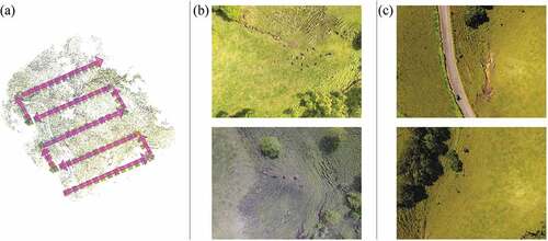
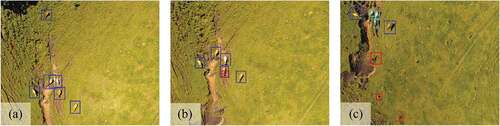
Dataset 2 contains 14 images taken on 24 August 2016 on one flight, and the weather was sunny and clear on this day, too. It was captured at a different area from Dataset 1 in the same pasture in Kumamoto, Japan. Images were photographed every 6 s in a stop-and-go manner. This dataset, with its different area and different season is used to test the robustness of our proposed cattle detection and counting system. (a) in Figure 1 shows one example of the flight routes. (b) and (c) in Figure 1 shows examples of images in both datasets.

Figure 1. Examples of flight route and images in our two datasets. (a) shows one example of flight route. (b) shows examples of dataset 1. (c) shows examples of dataset 2.

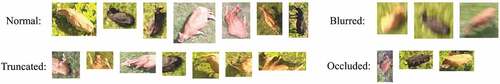
We manually annotated all the cattle in the images with the top-left position, width and height of the box enclosing them, a label illustrating the quality of the data, and the cattle IDs. The data quality labels include four types: (1) Normal – The whole target is in the image without blur, (2) Truncated – Cattle are at the edge of images and only part of the body is captured, (3) Blurred – The cattle are in blurred images, and (4) Occluded – Cattle have part of the body occluded. Several examples of each label in our datasets are given in Figure 2, and cattle in different poses, for example, walking and lying, are contained. For each flight, we labelled the same target in different images with the same ID and counted the number of individual targets in each flight area. Flights F and G in Dataset 1 contain two to five times more images than the others, so we divided the straight part of the flight routes into several flight sections, F-1 to F-8 and G-1 to G-8, in our experiment. The covered areas of each flight section vary from 1.5 to 5 hectares.

Figure 2. Examples of cattle with different labels in our datasets. Cattle in different poses (e.g., walking, lying) are included.

Dataset 1 contains 1886 annotations of 212 individual targets, and Dataset 2 contains 62 annotations of 6 individual targets. The median of cattle size is $87\times 90$ pixels in Dataset 1, and $59\times 101$ pixels in Dataset 2. The histogram of the length of the longer edge of the cattle bounding boxes with the data quality label Normal in Dataset 1 is shown in Figure 3. Among the 218 individual targets, 210 of them appeared more than once in the images. We assessed the moving distance of cattle during each flight section using the body length as a standard, and the overall statistics are shown in Table 1.

Table 1. Statistics of moving distance of 210 cattle that appear more than once in each flight section, which is estimated using body length as the denomination.

Moving distance (pixels)/body length (pixels)	0–1	1–2	2–3	3–4	4–5	5 –
Number of cattle	189	10	1	1	0	9

Figure 3. Histogram of longer edge of cattle bounding boxes with the data quality label Normal in Dataset 1.

The two datasets and corresponding annotations will be released at http://bird.nae-lab.org/cattle/.

3. Methods

3.1. System overview

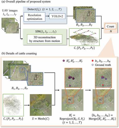
Figure 4 shows the overall pipeline of the proposed system. Its input is a sequence of images captured by a UAV, and its output is the number of individual targets that appear in that sequence. As the figure shows, the algorithm takes the following steps: 1) we detect cattle in each image, and 2) we also reconstruct the 3D surface of the pasture by SfM from the same set of images. With the candidate bounding boxes, the 3D surface, and the relative position of the cameras, 3) we merge the per-frame detection results guided by the 3D surface. Through this merging over time, the double detection of single cows are eliminated and we obtain the correctly counted number of cows.

Figure 4. Flowchart of cattle detection and counting system. A series of UAV images are fed to cattle detection and 3D surface reconstruction of the pasture. Then, we merge the per-frame detection results guided by the 3D surface to obtain correct counting of the targets.

More specifically, $\{I_1,I_2,...,I_T\}$ denotes the sequence of input images, and $B_t$ whose size is $N_t$ is a set of detected bounding boxes in image $I_t$. Three-dimensional reconstruction of the input images by SfM outputs $C$, a 3D point cloud, and $\{P_1,P_2,...,P_T\}$, which are camera parameters of corresponding images. Using the surface $S$, which is acquired by surface reconstruction of the point cloud, and the camera’s parameters $P_t$, we calculate ${B_t}^{\prime }$, the three-dimensional coordinates of each bounding box in image $I_t$. Finally, ${B_t}^{\prime }$ in each image are merged into $B$ to avoid duplicated counting of individual targets, and the size of the merged set $B$ estimates the number of targets $N$. The algorithm is formulated as follows to show the input and output of each step:

(1a) $B_t=\{b_{t,1},b_{t,2},...,b_{t,N_t}\}=\mathrm{D}\mathrm{e}\mathrm{t}\mathrm{e}\mathrm{c}\mathrm{t}(I_t)(t=1,2,...,T),$(1a)

(1b) $(C,\{P_1,P_2,...,P_T\})=\mathrm{S}\mathrm{f}\mathrm{M}(I_1,I_2,...,I_T),$(1b)

(1c) $S=\mathrm{M}\mathrm{e}\mathrm{s}\mathrm{h}(C),$(1c)

(1d) ${B_t}^{\prime }=\{{b_{t,1}}^{\prime },{b_{t,2}}^{\prime },...,{b_{t,N_t}}^{\prime }\}=\mathrm{R}\mathrm{e}\mathrm{p}\mathrm{r}\mathrm{o}\mathrm{j}\mathrm{e}\mathrm{c}\mathrm{t}(B_t;S,P_t)(t=1,2,...,T),$(1d)

(1e) $B=\{b_1,b_2,...,b_N\}=\mathrm{M}\mathrm{e}\mathrm{r}\mathrm{g}\mathrm{e}({B_1}^{\prime },{B_2}^{\prime },...,{B_T}^{\prime }).$(1e)

We discuss the details of Equation (1a) in 3.2, Equations (1b–1d) in 3.3.1, and Equation (1e) in 3.3.2.

3.2. Resolution optimization when detecting with yolov2

In general image recognition, the size of the target object in an image changes variously. In case there is a dramatic scale difference, scale-invariant/equivariant CNNs may be useful (Xu et al. 2014; Marcos et al. 2018). However, in this paper, UAV images are captured while maintaining the UAV at an approximately constant height. Therefore, it is possible to predict the resolution of the object to some extent. In this case, we show that a more suitable input resolution can be decided by this and by the network down-sampling rate.

While our system can be built with arbitrary cattle detectors, we specifically select YOLOv2 (Redmon and Farhadi 2017). YOLOv2 has some preferable properties to build systems for real-world applications: It runs near real-time using a single GPU, and its detection accuracy is near state-of-the-art in middle-scale benchmarks such as PASCAL VOC (Everingham et al. 2012) and MS COCO (Lin et al. 2014). It is pre-trained on ImageNet (Deng et al. 2009), and the pre-training plays an important role in detector accuracy (He, Girshick, and Dollár 2018; Agrawal, Girshick, and Malik 2014) and generalizability when training data is small (e.g., $<$10k MS COCO images) (Razavian et al. 2014). Another option in model selection is to design a slimmer model that specializes in cattle detection to pursuit further efficiency. Such model may be obtained by the model compression methods (Cheng et al. 2018) such as knowledge distillation (Hinton, Vinyals, and Dean 2014) and pruning (Han, Mao, and Dally 2016).

YOLOv2 contains 23 convolutional layers and five pooling layers, and its outline is shown in Figure 5. YOLOv2 inputs the entire image to the convolution layer, which means the calculation of the feature map only need to be performed once for the entire image. This is considered to be efficient because cattle only occupy a small part of the whole image. After the convolutional and pooling layers, an $W_{\mathrm{I}}\times H_{\mathrm{I}}$ input image is down-sampled into a $(W_{\mathrm{I}}/M)\times (H_{\mathrm{I}}/M)$ feature map. YOLOv2 predicts the positions and sizes of the objects from the output feature map using a $1\times 1$ convolutional layer.

Figure 5. Outline of YOLOv2 network (Redmon and Farhadi 2017). An $W_{\mathrm{I}}\times H_{\mathrm{I}}$ input image is down-sampled into a $(W_{\mathrm{I}}/M)\times (H_{\mathrm{I}}/M)$ feature map by the network. Several bounding boxes are predicted from each cell of the output feature map.

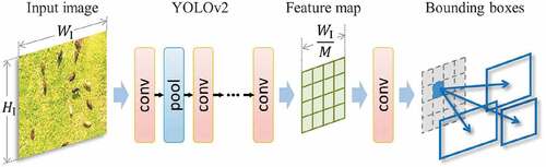
Since in YOLOv2 the regression that predicts the position of the bounding box is processed on each cell of the output feature map (Redmon and Farhadi 2017), we can expect better detection performance when the cell’s size is equal to the object’s, i.e., the regression is more effective when the cell size is adjusted to the size of the target. This is because if the cell is larger, it suffers from multiple objects inside it, and if it is smaller, multiple bounding boxes of one object will be predicted from multiple cells.

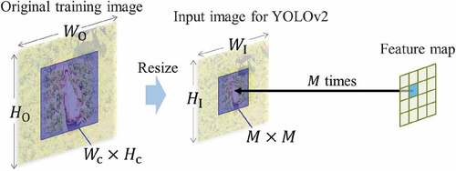
If the network down-samples an image by $M$, we resize the original training image in advance to make the size of the target objects equal to $M\times M$, as shown in Figure 6. When the size of a target is $W_{\mathrm{C}}\times H_{\mathrm{C}}$ in an $W_{\mathrm{O}}\times H_{\mathrm{O}}$ original training image, the optimal input resolution $W_{\mathrm{I}}\times H_{\mathrm{I}}$ can be calculated as

(2a) $W_{\mathrm{I}}=\frac{W_{\mathrm{O}}M}{W_{\mathrm{C}}},$(2a)

(2b) $H_{\mathrm{I}}=\frac{H_{\mathrm{O}}M}{H_{\mathrm{C}}},$(2b)

Figure 6. Resolution optimization. $W_{\mathrm{O}}\times H_{\mathrm{O}}$ denotes the size of the original training image, and the cattle size within it is $W_{\mathrm{C}}\times H_{\mathrm{C}}$. $W_{\mathrm{I}}\times H_{\mathrm{I}}$ denotes the size of the input image for YOLOv2 and $M$ is the down-sampling rate of the network. We resize an original $W_{\mathrm{O}}\times H_{\mathrm{O}}$ training image to $W_{\mathrm{I}}\times H_{\mathrm{I}}$ so that the size of the target object equals the size of one cell in the output feature map.

Accordingly, when an input image for YOLOv2 is down-sampled to a $C\times D$ feature map, $CM\times DM$ closest to $W_{\mathrm{I}}\times H_{\mathrm{I}}$ is the optimized resolution.

3.3. Merging detection results for counting

In order to accurately count the number of cattle located in a vast pasture, recognizing the same one appearing in multiple overlapped images is an essential task. Since pastures are often located in hilly countryside environments, stitching multiple overlapping images assuming a two-dimensional plane tends to fail, because the error by assuming a plane for the terrain to calculate homography is not negligible. For example, in our setting where the flight height is around 50 m and the diagonal angle of view is ${94}^{\circ }$, the error between the predicted (assuming a plane) and actual positions of the individual target can be up to four times the size of it, supposing that the actual position of the target is 5 m closer to the camera from the assumed plane. The actual terrain includes at most a 20 m height variance in our images. As a result, a target may appear twice in the stitched image or may disappear because it is covered by another image. Therefore, we assume cattle to be motionless and reconstruct a three-dimensional model for each area by SfM (Wu et al. 2011). We calculate all the positions of the detection results in the coordinate system of the reconstructed three-dimensional model and merge those detection results close to each other as the same target following the time sequence of photographing. Figure 4(b) provides a detailed overview of the cattle-counting part.

3.3.1. Calculating three-dimensional coordinates of detection results

Due to image capturing by a moving UAV, each image in the input sequence is from a different viewpoint, focal position, and camera pose. In the $t$-th image, given a 3D point $\mathit{q}=(X,Y,Z{)}^{\mathrm{T}}$ in the world coordinate and camera parameters $P_t$ including intrinsic matrix ${\mathbf{K}}_t$, rotation matrix ${\mathbf{R}}_t$, and translation vector ${\mathit{t}}_t$, the corresponding point in the image’s local coordinate $(x,y,z{)}^{\mathrm{T}}$ and its projection to the image $(u,v)$ can be calculated as follows:

(3a) $\left(\begin{array}{c}x\\ y\\ z\end{array}\right)={\mathbf{K}}_t({\mathbf{R}}_t\mathit{q}+{\mathit{t}}_t),$(3a)

(3b) $\left(\begin{array}{c}u\\ v\\ 1\end{array}\right)=\left(\begin{array}{c}x/z\\ y/z\\ 1\end{array}\right).$(3b)

Inversely, to recover 3D positions of the detection results, which are in the images’ local coordinates, we have to solve Equations (3.3.1) for $\mathit{q}$, as follows:

(4) $\mathit{q}={\mathbf{R}}_t^{-1}(z{\mathbf{K}}_t^{-1}\left(\begin{array}{c}u\\ v\\ 1\end{array}\right)-\mathit{t}{ }_t).$(4)

Here ${\mathbf{K}}_t$, ${\mathbf{R}}_t$, and ${\mathit{t}}_t$ are known from the output of SfM. To calculate the three-dimensional coordinates $\mathit{q}$ of the detection results in each image, we need to obtain the value of $z$ in Equation (4).

Three-dimensional models of each area are reconstructed by VisualSFM (Wu et al. 2011; Wu 2013). SIFT (Lowe 2004) is used to find pairs of feature points that are considered to be identical across images. Having matched the features, the three-dimensional shape and camera parameters are estimated by bundle adjustment (Wu et al. 2011). Furthermore, we conduct dense reconstruction by Furukawa’s CMVS/PMVS software (Furukawa et al. 2010; Furukawa and Ponce 2010). The output contains the three-dimensional coordinates of the point cloud $C$ and camera parameters $P_t$ of each image. We use screened poisson surface reconstruction (Kazhdan and Hoppe 2013), a surface reconstruction algorithm implemented in Meshlab (Cignoni et al. 2008) to create the surface $S$ from the point cloud.

The $z$ value of each pixel of the images can be obtained by rendering the surface $S$ from the perspective of cameras derived from $P_t$ and then reading its $z$-buffer, using OpenGL libraries (Segal and Akeley 2017). Suppose that the centre of a detection box $b_{t,i}$ in the $t$-th image is $(u,v)$; then, with the obtained $P_t$ and $z$ values, we can calculate the world coordinate $\mathit{q}$ using Equation (4).

3.3.2. Merging detection results along photographing time sequence

After calculating all the three-dimensional coordinates of the detection results, we merge the results considered to be the same target by Algorithm 1.

Algorithm 1 $Merge({B_1}^{\prime },{B_2}^{\prime },...,{B_T}^{\prime })$

Input: ${B_1}^{\prime },{B_2}^{\prime },...,{B_T}^{\prime }$

Output: $B=\{b_1,b_2,...,b_N\}$

B ← $\mathrm{\varnothing }$

for $t=1$ to $T$ do

if $B==\mathrm{\varnothing }$ then

Add all ${b_{t,i}}^{\prime }\in {B_t}^{\prime }$ to $B$

else

Calculate distance matrix ${\mathbf{M}}_{\mathrm{d}\mathrm{i}\mathrm{s}\mathrm{t}}$ whose ($i$, $j$) element is defined by the distance between ${b_{t,i}}^{\prime }$ and $b_j$

assignments $=$ hungarian(${\mathbf{M}}_{\mathrm{d}\mathrm{i}\mathrm{s}\mathrm{t}}$, threshold)

for all $(j,i)\in$ assignments do

b_j ← ${{\mathrm{b}}_{\mathrm{t},\mathrm{i}}}^{\prime }$

end for

for all $i$ such that (*, $i$) $\notin$ assignments do

Add ${b_{t,i}}^{\prime }$ to $B$

end for

end if

end for

return B

For each image, we use the Hungarian method (Miller, Stone, and Cox 1997; Munkres 1957), which solves the assignment problem, for matching detection results in each frame to the existing cattle list. The distance matrix ${\mathbf{M}}_{\mathrm{d}\mathrm{i}\mathrm{s}\mathrm{t}}$ containing distances between detection results in the new frame and the existing ones serve as the cost matrix in the assignment problem, and the threshold is used here as the cost of not assigning detection to any one in the existing cattle list. We replace the coordinate of the target in each assignment with the recent one, and the unassigned detection results are added to the list.

4. Experiments and results

4.1. Cattle detection

We used Darknet (Redmon 2013–2016) as the framework for training YOLOv2 (Redmon and Farhadi 2017). A total of 245 images in Dataset 1 were selected as training images. We use rotation for data augmentation to get more samples for cattle lying in a different direction in images, since in UAV images cattle can lie down in every direction, i.e., angle of the body to the horizontal line in the image can be various. First, each $4,000\times 3,000$ pixel image is cropped from both ends to $3,000\times 3,000$ pixels to obtain two overlapping square images. Then, for the two square images, we rotate on the area of $2,122\times 2,122$ pixels in the left one by multiple of ${30}^{\circ }$, and on the right one by ${15}^{\circ }$ plus multiple of ${30}^{\circ }$, obtaining 12 augmented images from each square image, and a total of 5,880 training images were obtained. The resolution of the original training image is $W_{\mathrm{O}}=H_{\mathrm{O}}=2,122$ and the median of cattle size is $W_{\mathrm{C}}=87$, $H_{\mathrm{C}}=90$. The down-sampling rate of YOLOv2 is $M=32$. Therefore, for input image sizes for YOLOv2, $W_{\mathrm{I}}=781$, $H_{\mathrm{I}}=754$ were calculated by Equations (3.2). We set the input resolution of training and testing images to $768\times 768$ pixels (size of the output feature map is $24\times 24$). The procedure of resizing the original input images into an input image for YOLOv2 is already implemented in the Darknet framework, and we set the resolution of the input image to our proposed resolution of $768\times 768$ in the configuration file for training.

Our training is a fine-tuning of YOLOv2 with pretraining using ImageNet (Deng et al. 2009), and there is only one class ‘cattle’ in our fine-tuning. The training was conducted for 4,000 iterations with one GeForce GTX TITAN X GPU. The learning rate was set at 0.001 after a burn-in of 200 iterations and reduced by a factor of 0.1 at iterations of 2,000 and 3,000. To show the difference more clearly between each input resolution, we did not use the multi-scale training¹ in YOLOv2, i.e., the input resolution is set to the same value throughout the training. As for testing, we cut the original images from the four corners into the same size as the training image ($2122\times 2122$ pixels) as testing images. Results of the four overlapping images are merged into the original image’s result by calculating the Intersection over Union (IOU) between those bounding boxes, and the threshold is 0.5.

For evaluation, we used the IOU of the detection results and the ground truth, and the threshold of IOU as a true positive (TP) is 0.2. In addition, we penalized multiple detection of the same animal, i.e., if there are two detection results whose IOU with the same ground truth is larger than the threshold, only the one with the larger IOU is evaluated as TP, and the other one is evaluated as a false positive (FP). Precision and recall are calculated while varying the confidence threshold using the numbers of TP, FP, and false negative (FN) in each testing image as follows:

(5) $\mathrm{P}\mathrm{r}\mathrm{e}\mathrm{c}\mathrm{i}\mathrm{s}\mathrm{i}\mathrm{o}\mathrm{n}=\frac{\mathrm{T}\mathrm{P}}{\mathrm{T}\mathrm{P}+\mathrm{F}\mathrm{P}},$(5)

(6) $\mathrm{R}\mathrm{e}\mathrm{c}\mathrm{a}\mathrm{l}\mathrm{l}=\frac{\mathrm{T}\mathrm{P}}{\mathrm{T}\mathrm{P}+\mathrm{F}\mathrm{N}},$(6)

(7) $F\text{-}\mathrm{m}\mathrm{e}\mathrm{a}\mathrm{s}\mathrm{u}\mathrm{r}\mathrm{e}=\frac{2\times \mathrm{P}\mathrm{r}\mathrm{e}\mathrm{c}\mathrm{i}\mathrm{s}\mathrm{i}\mathrm{o}\mathrm{n}\times \mathrm{R}\mathrm{e}\mathrm{c}\mathrm{a}\mathrm{l}\mathrm{l}}{\mathrm{P}\mathrm{r}\mathrm{e}\mathrm{c}\mathrm{i}\mathrm{s}\mathrm{i}\mathrm{o}\mathrm{n}+\mathrm{R}\mathrm{e}\mathrm{c}\mathrm{a}\mathrm{l}\mathrm{l}}.$(7)

Experiments were also conducted with the input resolution of $416\times 416$ pixels, which is the default value of YOLOv2 without our resolution optimization and serves as the baseline, and $1,184\times 1,184$ pixels, and several resolutions close to $768\times 768$ pixels. We first tested with the remaining 411 images in Dataset 1. The detection performances of different input resolutions are compared in Figure 7. Results with our optimized input resolution of $768\times 768$ pixels were significantly better than those with $416\times 416$ pixels and $1,184\times 1,184$ pixels, while similar results were achieved with input resolutions close to $768\times 768$ pixels. Also, as the zoomed part of high-recall areas shows, we can see that with the input resolution of $768\times 768$ pixels we obtain high precision around 0.95 with a high recall at 0.9.

Figure 7. Precision-recall curve of cattle detection at different input resolutions. Our proposed input resolution ($768\times 768$ pixels) achieved the best performance.

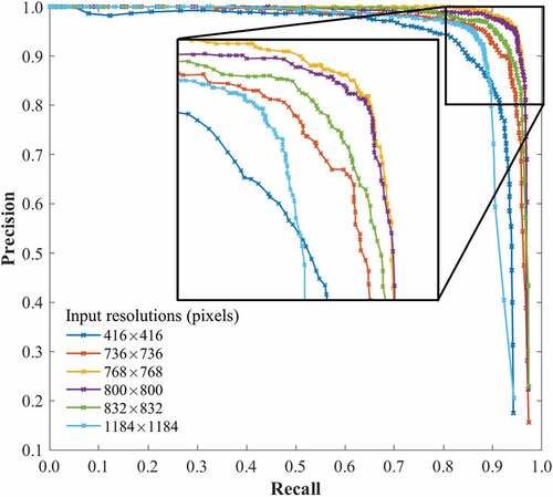
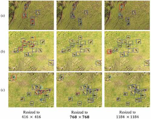
Although the performances of input resolutions around $768\times 768$ pixels are similar, the Area Under Curve (AUC) of the precision-recall curves in Figure 7 (listed in Table 2) demonstrate that when resizing the input resolution to $768\times 768$ pixels in accordance with the proposed resolution optimization, the best performance is obtained. Moreover, the highest F-measure was also achieved with this resolution and with the confidence threshold of 0.31. In this case, precision is 0.957, recall is 0.946, and F-measure is 0.952. In Figure 8, several detection results with different input resolutions (both in training and testing) are shown. FPs and FNs decreased as a result of our resolution optimization, especially in places where cattle are crowded.

Table 2. AUCs of different input resolutions.

Input resolution (pixels)	Area under the curve
$416\times 416$ (baseline)	0.905
$736\times 736$	0.945
$768\times 768$	0.964
$800\times 800$	0.961
$832\times 832$	0.957
$1,184\times 1,184$	0.906

Figure 8. Detection results (blue: TP, red: FP, cyan: FN). FP and FN decreased by using our proposed input resolution of $768\times 768$pixels. Examples of three areas are cropped from original images. The size of images in (a) is $1700\times 1100$ pixels. The size of images in (b) is $1700\times 1500$ pixels. The size of images in (c) is $1700\times 1300$ pixels.

For cross-validation, we first altered the training and testing data and achieved 0.941 precision, 0.944 recall, and 0.943 F-measure, which is close to the aforementioned results. We also conducted a three-split cross-validation in Dataset 1 with our optimized input resolutions of $768\times 768$ pixels, $416\times 416$ pixels, and $1,184\times 1,184$ pixels. The AUCs of precision–recall curves are shown in Table 3. Results of all the three splits consistently obtained the best performance with our proposed input resolution.

Table 3. AUCs of three-split cross-validation.

Input resolution (pixels)	Split 1	Split 2	Split 3
$416\times 416$	0.683	0.900	0.798
$768\times 768$	0.869	0.951	0.922
$1,184\times 1,184$	0.668	0.941	0.906

We also tested with Dataset 2, which was captured at a different area and different season than the training images. The precision of 0.774, recall of 0.661, and F-measure of 0.713 were achieved. Examples of detection results in Dataset 2 are shown in Figure 9, and we summarize the scores of our two datasets in Table 4. Our detection system performed well when the training and testing images were from the same dataset. Even when images contained some unknown background, which is the case in Dataset 2 and represents a much trickier situation, our detection system achieved the F-measure of 0.713.

Table 4. Detection results in different situations. When training and testing images are from the same dataset, i.e., when they have the same cattle size, high scores are achieved.

	Precision	Recall	F-measure
Training: Dataset 1	0.957	0.946	0.952
Testing: Dataset 1
Training: Dataset 1	0.774	0.661	0.713
Testing: Dataset 2

Figure 9. Detection results of Dataset 2 (blue: TP, red: FP, cyan: FN). (a) and (b) show typical examples of applying the detection system to a new area. (c) shows an example of problematic detection results that cattle counting suffer from.

4.2. Cattle counting

We reconstructed the three-dimensional model and the surface of the ground for all eight flights in the two datasets. In Figures 10 and 11, (a) shows examples of the feature points in the three-dimensional model, which are outputs of VisualSFM (Wu et al. 2011; Wu 2013), and (b) shows the results of the surface reconstruction by screened poisson surface reconstruction (Kazhdan and Hoppe 2013) in Meshlab (Cignoni et al. 2008).

Figure 10. Visualization of each step in cattle counting. (a) Feature points in 3D model output by VisualSFM (Wu et al. 2011; Wu 2013). (b) Surface reconstruction result by screen poission surface reconstruction (Kazhdan and Hoppe 2013) in Meshlab (Cignoni et al. 2008). (c) Visualization of all detection results. (d) Visualization of merged results. Line (i) is the results of flight section B and line (ii) is the results of flight section G-4 in Dataset 1, which are examples of (i) Motionless. In (c), detection results of the same target are close to each other. Transparency of ground surface in (c) and (d) is adjusted for visualization of three-dimensional coordinates of detection results and ground truth.

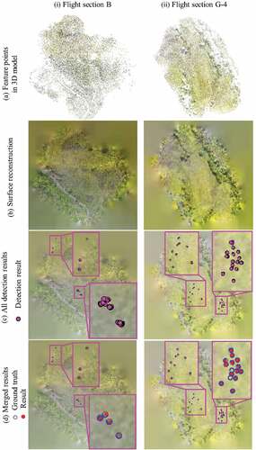
Figure 11. Results of (II) Moving. Line (i) is the results of flight section C and line (ii) is the results of flight section E in Dataset 1. In flight section C, cattle moved so long a distance during the photographing that we could not merge the detection results correctly. In flight section E, we can see the moving route of cattle in (c), and in (d), they are merged. The explanation of (a) to (d) is the same as in Figure 10.

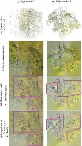
The three-dimensional coordinates of the detection results were calculated and merged. The threshold used in the merging depended on the scale of the three-dimensional models, and the value we used here is 0.05. We visualized the merged results and the ground truth together with the reconstructed surface and evaluate the results with Missed – the number of missed cattle, Double Count – the number of double counts and Not Cattle – the number of results that are not cattle, by comparing the visualized results and images with detection results. As (c) and (d) in Figures 10 and 11 show, the detection results located close to each other are merged into the same target.

The counting results of flight sections in Dataset 1 are shown in Tables 5 and 6. Since cattle are assumed to keep motionless during photographing, flight sections are divided into two groups based on moving distance of the cattle, specifically, (I) Motionless: moving distances of all cattle during the flight section were less than their body length, and (II) Moving: cattle that have moved more than their body length during the flight section exist. In the case of (I) Motionless, as shown in Table 5, we count cattle with high precision. The error of our count results in each flight section is up to 3 and the numbers of Double Count for all flight sections are all 0, while that of Missed, and Not Cattle are up to 3 for dozens of cattle. As for (II) Moving, as shown in Table 6, in some flight sections, results that are about 1.5 times of the true value are observed.

Table 5. Counting results of dataset 1. (I): Motionless: Moving distances of all cattle during the flight section were less than their body length. The number of missed, double count and not cattle are small. Counting result close to true value is achieved.

Flight section	No. true	No. our count	No. missed	No. double count	No. not cattle
A	4	5	0	0	1
B	7	7	0	0	0
F-1	8	8	0	0	0
F-2	20	19	1	0	0
F-4	20	20	0	0	0
F-5	14	14	0	0	0
F-6	0	0	0	0	0
F-7	0	1	0	0	1
F-8	0	1	0	0	1
G-1	2	2	0	0	0
G-2	17	15	2	0	0
G-3	25	23	3	0	1
G-4	25	22	3	0	0
G-6	5	5	0	0	0
G-7	0	1	0	0	1
G-8	0	0	0	0	0
Sum	147	143	9	0	5

Table 6. Counting result of dataset 1. (II) Moving: Cattle that have moved more than their body length during the flight section exist.

Flight section	No. true	No. our count	No. missed	No. double count	No. not cattle
C	12	18	7	13	0
D	5	7	1	2	1
E	5	8	0	1	2
F-3	24	24	0	0	0
G-5	19	17	3	0	1
Sum	65	74	11	16	4

We also counted cattle in the area of Dataset 2, which belongs to (II) Moving. The images in this dataset were captured at 6-s intervals, which is three times as long as in Dataset 1, so when merging the detection results, we set the threshold of distance to three times the value used in the experiment on Dataset 1. Results of Dataset 2 are listed in Table 7.

Table 7. Counting result of dataset 2. This flight belongs to (II) Moving.

Flight section	No. true	No. our count	No. missed	No. double count	No. not cattle
Dataset 2	6	12	3	3	6

5. Discussion

In terms of cattle detection, our method of applying resolution optimization to detection by YOLOv2 performed well, which laid the groundwork for cattle counting by merging the detection results. From Figure 7, we can see that the detection performance with our proposed resolution of $768\times 768$ pixels is significantly higher than the result with $416\times 416$ pixels and $1,184\times 1,184$ pixels. However, although we set the multi-scale training off, the results with resolutions close to $768\times 768$ pixels still did not show much difference between each other. Considering that the pasture is located in a hilly countryside environment and that the flight height of the UAV is set by the altitude, the distance from the ground may change during the photographing, which will lead to slight variations of cattle size. Therefore, the results close to the optimized one are similar and are significantly higher than input resolutions that are several times larger or smaller.

We also utilized our system to detect cattle in Dataset 2, which contains images captured at different area from the training images as well as different sizes of cattle. As shown in Table 4, the results of testing images with a different background from the training images are lower than the case where training and testing images were captured in the same areas and from the same flight height. Thus, adding more training images that contain different backgrounds in the future might make the system more robust. Moreover, future investigation into varying the resolution of testing images adaptively might also be one of our future work.

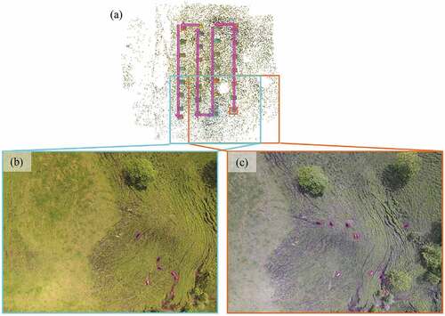
As for cattle counting, the results of motionless cattle are close to true value, and the instances of Missed, Double Count, and Not Cattle are few. Although our proposed counting method, which merges the detection results by distance in a three-dimensional model and replaces the coordinate of an individual target with the latter one along the photographing time sequence, succeeded in merging the results of the same target that is motionless or continuously appears in all the images in the time sequence, it failed to merge when an individual target appears intermittently in images and moves significantly when it is outside the image. For example, in flight section C in Dataset 1 (line (i) in Figure 11), the number of Double Count is 13, while the true value of cattle is 12. The two images (b) and (c) highlighted in Figure 12 indicate that the position of cattle changed significantly while the UAV was flying to the other end of the area and coming back. In addition, there are images between the highlighted two that do not contain those moving cattle. As a result, our method failed to merge these detection results, which resulted in 13 double counts.

Figure 12. The flight route and two of the images in flight section C in Dataset 1. In (a) the flight route is indicated by arrows and in (b) and (c) the positions of cattle in the images are highlighted by magenta boxes. (b) is rotated ${180}^{\circ }$ for comparison with (c). By comparing (b) and (c), we can see that cattle moved long distances during the drone’s zigzag flight.

Furthermore, the number of Not Cattle directly suffers from the FPs in the detection results. For example, in (a) of Figure 9, there are three FPs, which are actually grass as the background, so it added three Not Cattle in the counting result of Dataset 2. As for the number of Missed, since we use the position at which cattle last appeared during the flight as ground truths if a target keeps moving and we fail to detect it in the last image in which it appears, it turns out to be a missed one in the counting result. Therefore, as future work, improving the detection performance should lead to higher counting precision, especially when applying our system to counting cattle in a pasture different from the one of the training images.

6. Conclusion

In this study, we proposed a cattle detection and counting system using UAV images. Considering the feature of UAV images that the targets all appear with almost the same size when the flight height is fixed, we resized the training images to the resolution where the size of cattle is equal to the size of one cell in the output feature map. Detection performance was improved by the input resolution optimization, and we obtained a precision of 0.957, a recall of 0.946, and a 0.952 F-measure . As for counting cattle in a vast area of 1.5 to 5 hectares, when all cattle move less than their body length during the flight section, results close to the true value were obtained.

Since detection performance decreases when applying our system to Dataset 2, making the system more robust to a new area is one of our future works. Increasing the training data to include different backgrounds and seasons is one avenue to explore. In addition, introducing the idea of domain adaptation may also be promising for increasing the performance on a slightly differently dataset.

Our cattle detection and counting system can also be applied to other slow-moving animals, as well. However, the performance would descend when counting fast-moving animals. In our experiments, the counting results of flight sections that contain cattle whose moving distances are longer than their body length need to be improved in the future. Also, it is difficult to merge results of different flight sections split from one flight by our system, since during the whole flight some of the targets walked to the former position of the other one. For these limitations, re-identification using the feature of each target, e.g., the pattern of the animals skin and the figure of the animals body can be considered in the future.

Acknowledgements

We thank the Emergency medical and Disaster coping Automated drones support system utilization promotion Council (EDAC) for their cooperation with the UAV image capturing.

Disclosure statement

No potential conflict of interest was reported by the authors.

Additional information

Funding

This work was supported by grants from the Japan Society for the Promotion of Science [JP16J04552,JP18K11348].

Notes

1. An implement in YOLOv2, by which input resolution is randomly chosen every 10 iterations except the last 200, in the range of 10 resolutions around the value.

References

- Agrawal, P., R. Girshick, and J. Malik. 2014. “Analyzing the Performance of Multilayer Neural Networks for Object Recognition.” In Computer Vision – ECCV 2014, edited by D. Fleet, T. Pajdla, B. Schiele, and T. Tuytelaars, 329–344. Cham: Springer International Publishing.
- Ardã, H., O. Guzhva, M. Nilsson, and A. H. Herlin. 2018. “Convolutional Neural Network-Based Cow Interaction Watchdog.” IET Computer Vision 12 (2): 171–177. doi:10.1049/iet-cvi.2017.0077.
- Chamoso, P., W. Raveane, V. Parra, and G. Angélica. 2014. “UAVs Applied to the Counting and Monitoring of Animals.” In Ambient Intelligence - Software and Applications, edited by C. Ramos, P. Novais, C. E. Nihan, and J. M. Corchado Rodríguez, 71–80. Cham: Springer International Publishing.
- Cheng, Y., D. Wang, P. Zhou, and T. Zhang. 2018. “Model Compression and Acceleration for Deep Neural Networks: The Principles, Progress, and Challenges.” IEEE Signal Processing Magazine 126–136. doi:10.1109/MSP.2017.2765695.
- Chrtien, L.-P., J. Thau, and P. Mnard. 2016. “Visible and Thermal Infrared Remote Sensing for the Detection of White-Tailed Deer Using an Unmanned Aerial System.” Wildlife Society Bulletin 40 (1): 181–191. https://onlinelibrary.wiley.com/doi/abs/10.1002/wsb.629
- Cignoni, P., M. Callieri, M. Corsini, M. Dellepiane, F. Ganovelli, and G. Ranzuglia. 2008. “MeshLab: An Open-Source Mesh Processing Tool.” In Eurographics Italian Chapter Conference, edited by V. Scarano, R. De Chiara, and U. Erra. Eurographics Association. Salerno, Italy.
- Cortes, C., and V. Vapnik. 1995. “Support-Vector Networks.” Machine-Learning 20 (3): 273–297. doi:10.1007/BF00994018.
- Dalal, N., and B. Triggs. 2005. “Histograms of Oriented Gradients for Human Detection.” In 2005 IEEE Computer Society Conference on Computer Vision and Pattern Recognition (CVPR’05), Vol. 1, June, 886–893. San Diego, CA, USA.
- Deng, J., W. Dong, R. Socher, L. Li, L. Kai, and L. Fei-Fei. 2009. “ImageNet: A Large-Scale Hierarchical Image Database.” In 2009 IEEE Conference on Computer Vision and Pattern Recognition, June, 248–255. Miami, FL, USA.
- Everingham, M., L. Van Gool, C. K. I. Williams, J. Winn, and A. Zisserman. 2012. “The PASCAL Visual Object Classes Challenge 2012 (VOC2012) Results.” http://www.pascal-network.org/challenges/VOC/voc2012/workshop/index.html
- Fang, Y., D. Shengzhi, R. Abdoola, K. Djouani, and C. Richards. 2016. “Motion Based Animal Detection in Aerial Videos.” Procedia Computer Science 92: 13–17. 2nd International Conference on Intelligent Computing, Communication & Convergence, ICCC 2016, 24-25 January 2016, Bhubaneswar, Odisha, India http://www.sciencedirect.com/science/article/pii/S1877050916315629
- Furukawa, Y., B. Curless, S. M. Seitz, and R. Szeliski. 2010. “Towards Internet-Scale Multi-View Stereo.” In 2010 IEEE Computer Society Conference on Computer Vision and Pattern Recognition, June, 1434–1441.
- Furukawa, Y., and J. Ponce. 2010. “Accurate, Dense, and Robust Multiview Stereopsis.” IEEE Transactions on Pattern Analysis and Machine Intelligence 32 (8): 1362–1376. doi:10.1109/TPAMI.2009.161.
- Gonzalez, L. F., G. A. Montes, E. Puig, S. Johnson, K. Mengersen, and K. J. Gaston. 2016. “Unmanned Aerial Vehicles (Uavs) and Artificial Intelligence Revolutionizing Wildlife Monitoring and Conservation.” Sensors 16: 1. doi:10.3390/s16122100.
- Han, S., H. Mao, and W. J. Dally. 2016. “Deep Compression: Compressing Deep Neural Networks with Pruning, Trained Quantization and Huffman Coding.” In International Conference on Learning Representations, San Juan, Puerto Rico.
- He, K., X. Zhang, S. Ren, and J. Sun. 2016. “Deep Residual Learning for Image Recognition.” In 2016 IEEE Conference on Computer Vision and Pattern Recognition (CVPR), June, 770–778. Las Vegas, NV, USA.
- He, K., R. B. Girshick, and D. Piotr 2018. “Rethinking ImageNet Pre-Training.” CoRR abs/1811.08883. http://arxiv.org/abs/1811.08883
- Hinton, G., O. Vinyals, and J. Dean. 2014. “Distilling the Knowledge in a Neural Network.” Deep Learning and Representation Learning Workshop in Conjunction with NIPS, Montreal, Canada.
- Hodgson, J. C., S. M. Rowan Mott, T. T. Baylis, S. W. Pham, A. D. Kilpatrick, R. R. Segaran, I. Reid, A. Terauds, and L. P. Koh. 2018. “Drones Count Wildlife More Accurately and Precisely than Humans.” Methods in Ecology and Evolution 9 (5): 1160–1167. https://besjournals.onlinelibrary.wiley.com/doi/abs/10.1111/2041-210X.12974
- Kazhdan, M., and H. Hoppe. 2013. “Screened Poisson Surface Reconstruction.” ACM Transactions on Graphics 32 (3): 29:1–29: 13. doi:10.1145/2487228.2487237.
- Kellenberger, B., M. Volpi, and D. Tuia. 2017. “Fast Animal Detection in UAV Images Using Convolutional Neural Networks.” In 2017 IEEE International Geoscience and Remote Sensing Symposium (IGARSS), July, 866–869. Fort Worth, Texas, USA.
- Kellenberger, B., D. Marcos, and D. Tuia. 2018. “Detecting Mammals in UAV Images: Best Practices to Address a Substantially Imbalanced Dataset with Deep Learning.” Remote Sensing of Environment 216: 139–153. doi:10.1016/j.rse.2018.06.028.
- Krizhevsky, A., I. Sutskever, and G. E. Hinton. 2012. “ImageNet Classification with Deep Convolutional Neural Networks.” In Proceedings of the 25th International Conference on Neural Information Processing Systems - Volume 1, NIPS’12, USA, 1097–1105. Curran Associates . http://dl.acm.org/citation.cfm?id=2999134.2999257
- Lhoest, S., J. Linchant, S. Quevauvillers, C. Vermeulen, and P. Lejeune. 2015. “How Many Hippos (HOMHIP): Algorithm for Automatic Counts of Animals with Infra-Red Thermal Imagery from UAV.” The International Archives of the Photogrammetry, Remote Sensing and Spatial Information Sciences XL-3/W3: 335–362.
- Lin, T.-Y., S. J. Michael Maire, L. D. Belongie, R. B. Bourdev, J. H. Girshick, P. Perona, D. Ramanan, P. Dollár, and C. Lawrence Zitnick. 2014. “Microsoft COCO: Common Objects in Context.” In European Conference on Computer Vision, 740–755. Zurich, Switzerland.
- Liu, W., D. Anguelov, D. Erhan, C. Szegedy, S. Reed, F. Cheng-Yang, and A. C. Berg. 2016. “SSD: Single Shot MultiBox Detector.” In Computer Vision – ECCV 2016, edited by B. Leibe, J. Matas, N. Sebe, and M. Welling, 21–37. Cham: Springer International Publishing.
- Liu, X., S. W. Chen, S. Aditya, N. Sivakumar, S. Dcunha, Q. Chao, C. J. Taylor, J. Das, and V. Kumar. 2018. “Robust Fruit Counting: Combining Deep Learning, Tracking, and Structure from Motion.” In IEEE/RSJ International Conference on Intelligent Robots and Systems, Madrid, Spain.
- Longmore, S. N., R. P. Collins, S. Pfeifer, S. E. Fox, M. Mulero-Pzmny, F. Bezombes, A. Goodwin, M. De Juan Ovelar, J. H. Knapen, and S. A. Wich. 2017. “Adapting Astronomical Source Detection Software to Help Detect Animals in Thermal Images Obtained by Unmanned Aerial Systems.” International Journal of Remote Sensing 38 (8–10): 2623–2638. doi:10.1080/01431161.2017.1280639.
- Lowe, D. G. 2004. “Distinctive Image Features from Scale-Invariant Keypoints.” International Journal of Computer Vision 60 (2): 91–110. doi:10.1023/B:VISI.0000029664.99615.94.
- Marcos, D., B. Kellenberger, S. Lobry, and D. Tuia. 2018. “Scale Equivariance in CNNs with Vector Fields.” In ICML/FAIM 2018 workshop on Towards learning with limited labels: Equivariance, Invariance, and Beyond, Stockholm, Sweden.
- Miller, M. L., H. S. Stone, and I. J. Cox. 1997. “Optimizing Murty’s Ranked Assignment Method.” IEEE Transactions on Aerospace and Electronic Systems 33 (3): 851–862. doi:10.1109/7.599256.
- Mundhenk, T., G. K. Nathan, W. A. Sakla, and K. Boakye. 2016. “A Large Contextual Dataset for Classification, Detection and Counting of Cars with Deep Learning.” In Computer Vision – ECCV 2016, edited by B. Leibe, J. Matas, N. Sebe, and M. Welling, 785–800. Cham: Springer International Publishing.
- Munkres, J. 1957. “Algorithms for the Assignment and Transportation Problems.” Journal of the Society for Industrial and Applied Mathematics 5 (1): 32–38. doi:10.1137/0105003.
- Oishi, Y., and T. Matsunaga. 2014. “Support System for Surveying Moving Wild Animals in the Snow Using Aerial Remote-Sensing Images.” International Journal of Remote Sensing 35 (4): 1374–1394. doi:10.1080/01431161.2013.876516.
- Razavian, A. S., H. Azizpour, J. Sullivan, and S. Carlsson. 2014. “CNN Features Off-the-Shelf: An Astounding Baseline for Recognition.” In Proceedings of the 2014 IEEE Conference on Computer Vision and Pattern Recognition Workshops, CVPRW ‘14, 512–519, Washington, DC, USA: IEEE Computer Society. doi: 10.1109/CVPRW.2014.131.
- Redmon, J., and A. Farhadi. 2017. “YOLO9000: Better, Faster, Stronger.” In IEEE Conference on Computer Vision and Pattern Recognition, 6517–6525. Honolulu, Hawaii, USA. doi:10.1109/CVPR.2017.690.
- Redmon, J. 2013–2016. “Darknet: Open Source Neural Networks in C.” http://pjreddie.com/darknet/
- Ren, S., K. He, R. Girshick, and J. Sun. 2017. “Faster R-CNN: Towards Real-Time Object Detection with Region Proposal Networks.” IEEE Transactions on Pattern Analysis and Machine Intelligence 39 (6): 1137–1149. doi:10.1109/TPAMI.2016.2577031.
- Rivas, A., P. Chamoso, A. Gonzlez-Briones, and J. M. Corchado. 2018. “Detection of Cattle Using Drones and Convolutional Neural Networks.” Sensors 18: 7. doi:10.3390/s18072048.
- Salberg, A. 2015. “Detection of Seals in Remote Sensing Images Using Features Extracted from Deep Convolutional Neural Networks.” In 2015 IEEE International Geoscience and Remote Sensing Symposium (IGARSS), July, 1893–1896. Milan, Italy.
- Schönberger, J. L., and J. Frahm. 2016. “Structure-from-Motion Revisited.” In 2016 IEEE Conference on Computer Vision and Pattern Recognition (CVPR), June, 4104–4113. Las Vegas, NV, USA.
- Segal, M., and K. Akeley. 2017. “The OpenGL Graphics System: A Specification, Version 4.5 (Core Profile).” https://www.khronos.org/registry/OpenGL/specs/gl/glspec45.core.pdf
- Tayara, H., K. Gil Soo, and K. T. Chong. 2018. “Vehicle Detection and Counting in High-Resolution Aerial Images Using Convolutional Regression Neural Network.” IEEE Access 6: 2220–2230. doi:10.1109/ACCESS.2017.2782260.
- Van Gemert, J. C., C. R. Verschoor, P. Mettes, K. Epema, L. P. Koh, and S. Wich. 2015. “Nature Conservation Drones for Automatic Localization and Counting of Animals.” In Computer Vision - ECCV 2014 Workshops, edited by L. Agapito, M. M. Bronstein, and C. Rother, 255–270. Cham: Springer International Publishing.
- Wu, C. 2013. “Towards Linear-Time Incremental Structure from Motion.” In International Conference on 3D Vision - 3DV, June, 127–134. Seattle, Washington, USA.
- Wu, C., S. Agarwal, B. Curless, and S. M. Seitz. 2011. “Multicore Bundle Adjustment.” In IEEE Conference on Computer Vision and Pattern Recognition, June, 3057–3064. Colorado Springs, CO, USA.
- Xu, Y., T. Xiao, J. Zhang, K. Yang, and Z. Zhang. 2014. “Scale-Invariant Convolutional Neural Networks.” CoRR abs/1411.6369. http://arxiv.org/abs/1411.6369