Vegetation mapping of No Name Key, Florida using lidar and multispectral remote sensing

ABSTRACT

LIght Detection And Ranging (lidar) data have been widely used in the areas of ecological studies due to lidar’s ability to provide information on the vertical structure of vegetation in wildlife habitats. The overall objective of this project was to map the vegetation on No Name Key, Florida where endangered wildlife species reside using publicly available remote sensing data such as lidar data and high resolution aerial images (including National Agricultural Imagery Program (NAIP) images). The methods involved the use of 4 different classification algorithms (Support Vector Machine, Random Forest, Maximum Likelihood, and Mahalanobis Distance), different classification settings (default and custom settings), and normalization (original and normalized input bands) on 2 different input stacked images, NAIP image alone and NAIP combined with lidar data. A majority filter was applied to each classification output before performing the accuracy assessment. The result of performing the image classifications showed the following: across all inputs and classification algorithms, the highest overall accuracy (OA) and kappa coefficient (к) were achieved by the Random Forest classification on the NAIP-lidar stacked image with an applied majority filter and original input bands. The result also showed the airborne data combined with the lidar data resulted in a higher classification accuracy than the airborne data alone; and when normalization was applied to all the input bands or layers, the classification accuracies were not increased in most cases compared to when original bands were used in the classification. In most cases, the application of the majority filter increased the accuracy of the classification results as opposed to when no majority filter was applied. Instead of using default values, when the new parameter values (i.e., custom settings) for the penalty parameter (C) and the gamma (ɤ) were used, the accuracies of the Support Vector Machine (SVM) classified images were slightly increased compared to using the default values for the 2 parameters. With increased availability of public lidar data, combining the aerial image with lidar data would enhance the accuracy of vegetation mapping, which would lead to more effective and accurate wildlife management.

1. Introduction

Accurate mapping of land use/land cover types would increase the understanding of natural resources and thus improve the management of endangered wildlife species. One technology that improves mapping is remote sensing, which refers to acquiring information on an object or a phenomenon without actual contact with it: an aerial photo is 1 example of remote sensing. One common use of remote sensing would be the creation of land use/land cover maps. This process is conducted by means of image classifications, a process of converting remotely sensed images into information or maps (Campbell and Wynne 2011; Jensen 2015). This process serves as a basis for all other remote sensing studies. There have been numerous studies which used remote sensing to create land use/land cover maps. For example, Boelman et al. (2016) applied remote sensing technology to accurately map the tundra breeding habitat of two songbird species to understand their habitat use and reproductive success. Bouchhima et al. (2018) used remote sensing to create a halophyte vegetation distribution map to study the distribution of halophytes and thus to understand the extent of salinization. Additionally, Haest et al. (2017) used the remote sensing approach to map and monitor protected habitat areas.

One form of remote sensing is lidar (LIght Detection And Ranging) technology, which uses laser light as its energy source. A lidar sensor measures the travel time (from the lidar instrument to the object and back to the sensor) and calculates the distance from the lidar instrument to the target. Lidar remote sensing is particularly useful because it provides information about elevation (i.e., vegetation height). It has been used in many ecological studies including wildlife habitat mapping, forest inventory, canopy dimension estimation, and aboveground biomass study. Srinivasan et al. (2014) used multi-temporal lidar data to model tree biomass change, and Putman and Popescu (2018) estimated dead standing tree volume by using lidar data.

Over the years, lidar data have been proven to improve land cover classification results when used in addition to multispectral remote sensing. Since lidar data provide information on the vertical structure of the vegetation and ground topography, it is important to use lidar data in vegetation mapping studies as well as multispectral data. There are a number of studies that used the data fusion technique of both lidar data and multispectral data in image classifications. For example, Mutlu, Popescu, and Zhao (2008) used the 2 different surface fuel maps in predicting fire behaviour in east Texas, one created by performing image classification on satellite imagery alone and the other created by performing image classification on the fused image of space-borne data combined with a lidar-derived dataset. The results of the study indicated the following: (1) the use of the lidar-derived dataset (such as canopy cover) greatly improved the accuracy of surface fuel map (by 13% or higher) compared to the use of satellite data alone, and (2) lidar-derived variables were able to provide more detailed information on fire characteristics, which led to more accurate modelling of fire behaviour and assessing fire risk (Mutlu, Popescu, and Zhao 2008). In addition, García et al. (2011) used both airborne data and lidar data in mapping different fuel types for forest fires. The authors utilized a 2 step process in fuel type mapping. In the first classification phase, the Support Vector Machine (SVM) algorithm was applied to the fused image of multispectral data and lidar derived products in order to discriminate among the main fuel groups. In the second classification phase, the decision tree algorithm was applied to the combined image of the SVM classification results and some of the lidar derived products to separate the additional fuel categories.

As discussed in García et al. (2011), lidar data provide information on height or vertical structure of the vegetation, which multispectral data alone cannot offer. This additional height information as well as the features or variables extracted from lidar can greatly help to classify vegetation (with similar spectral values) into different classes more accurately. Vegetation height information along with extracted features or variables from lidar were an integral part of the current study.

The study took place in the Lower Florida Keys, an environment which is characterized by multiple inter-related components, such as environmental elements, climate factors, and anthropogenic influences. In areas such as the Lower Florida Keys that have low lying coastal areas, ground topography, which lidar data provides, is important because different vegetation communities can be formed by subtle changes in elevation. Climate change may have a greater impact, especially on the low lying coastal environments, resulting in increased rates of relative sea-level rise and increased frequency and intensity of severe storms. The frequent and severe storms caused by climate change (Martínez et al. 2007) will likely have a devastating impact on low lying coastal vegetation communities. In addition to climate change impact on vegetation, increased human population in the Keys has resulted in more human-dominated areas (i.e., development and roads), leading to fragmentation and loss of habitat.

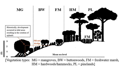
Conservation of the Lower Florida Keys environment is particularly important because of its unique and diverse flora and fauna. Once this particular environment is destroyed, the wildlife species inhabiting it will no longer be available for the enjoyment of future generations. Silvy (1975) and Lopez (2001) described the importance of environments as fundamental units, which then determine the fate of any endemic wildlife species belonging to the system. The environment of Lower Florida Keys, which consist of different vegetation types as well as many abiotic and biotic factors, are home to many wildlife species. Numerous endangered wildlife species, including Key deer (Odocoileus virginianus clavium), Lower Keys marsh rabbits (Sylvilagus palustris hefneri), and silver rice rats (Oryzomys palustris natator), reside in the Lower Florida Keys. All these wildlife species use at least 1 of the 6 vegetation types studied by Lopez et al. (2004) and arranged here from low to high elevations: mangrove, developed, buttonwood, freshwater marsh, hardwoods/hammocks, and pinelands. These 6 vegetation types all appear between 0–3 m above mean sea level (Lopez et al. 2004).

Considering the narrow vertical range in which each type of vegetation can grow (all vegetation types appear within the elevation range of 0–3 m above mean sea level), accurate vegetation mapping is particularly important in this region. Since coastal vegetation is adapted to live in a certain terrain elevation (in reference to mean sea water level) and a certain distance from the water, changes in terrain elevation (relative to the sea level) or slight distance changes from the water line can result in completely different vegetation communities. The accurate mapping of different vegetation types will help estimate the amount of particular vegetation types available to a certain wildlife species in the Keys, and the mapping will also help improve the conservation of various species such as Lower Keys marsh rabbits.

Despite the importance of the accurate vegetation mapping using the information from lidar data, studies suggest that variables or features derived from lidar data have not been used in the previous vegetation mapping projects of the Florida Keys. In the study by Lopez (2001) and Lopez et al. (2004), vegetation data from the Advanced Identification of Wetlands Project was used to create vegetation maps for the study area. A few years later, LaFever et al. (2007) used United States Geological Survey (USGS) Digital Elevation Model (DEM) and digitized vegetation map of the Lower Florida Keys from Faulhaber (2003) to calculate the proportion of each vegetation type. Recently, Svejkovsky et al. (2020) used NDVI (Normalized Difference Vegetation Index) data derived from spaceborne multispectral images to conduct change detection analysis. In Svejkovsky et al.’s study, the data were used to study the impact of Hurricane Irma on different vegetation types in the Lower Florida Keys and also to find out the spatial extent of vegetation recovery after the storm.

Machine learning algorithms (Random Forest and Support Vector Machine (or SVM)) as well as traditional algorithms can be used to classify vegetation types. A Random Forest algorithm can be viewed as an expansion of a ‘Decision Tree’ classifier. The Decision Tree classification is performed in multiple stages that are composed of a series of binary decisions to place a pixel into different classes. The Random Forest algorithm grows many ‘classification trees’ (Gislason, Benediktsson, and Sveinsson 2006) whose basic building block is a single Decision Tree. In the Random Forest classification, each ‘classification tree’ produces its own classification results, and the one that is most consistent across all the ‘classification trees’ would be the final classification result (Gislason, Benediktsson, and Sveinsson 2006). A few advantages of the Random Forest algorithm over other classification algorithms are that it provides good classification accuracy, it can handle large data sets, and it does not require the normality of the training data (Rodriguez-Galiano et al. 2012).

Machine learning methods, especially the Random Forest method, are commonly used to map different vegetation classes. Na et al. (2010) compared the image classification accuracies in mapping different land cover classes among 3 machine learning methods: Random Forest, Classification and Regression Trees (CART), and Maximum Likelihood. According to Na et al. (2010), the Random Forest method achieved the highest overall accuracy (OA) and kappa coefficient (к) compared to CART and Maximum Likelihood. The result also indicated that the Random Forest algorithm was least sensitive to the reduction in the number of training samples (Na et al. 2010). It was more robust in the presence of noise in the training data, thus providing an improvement over the other 2 methods in land cover classification (Na et al. 2010). The increased classification accuracy in mapping different land cover types compared to the accuracy of the Maximum Likelihood classification is discussed in many other studies, such as Rodriguez-Galiano et al. (2012).

The Support Vector Machine (SVM) algorithm, another machine learning method that is frequently used to classify land cover classes, separates classes with a decision surface that maximizes the margin between different classes (Mountrakis, Im, and Ogole 2011). An example of the simplest SVM classification would be a case with 2 classes, and the SVM classifier would act as a binary classifier, which assign the dataset into 1 of the 2 classes (Mountrakis, Im, and Ogole 2011). In cases when the separation between classes is difficult and complex, a kernel transformation can be used. By using the kernel transformations, the input space is transformed into a higher dimension, in which the separation between classes is simpler and easier (Mountrakis, Im, and Ogole 2011). A few advantages of the SVM algorithm over other classification methods are that it performs well, even when the limited number of training sample is available, and it does not require the normality of the training data (Mountrakis, Im, and Ogole 2011).

The SVM algorithm is frequently used to map land cover classes. García et al. (2011) compared the SVM classification with Maximum Likelihood and found that the accuracy of the SVM classification was higher than the Maximum Likelihood classification accuracy. Ustuner, Sanli, and Dixon (2015) used 63 SVM models consisting of different combinations of internal parameters. Four kernel types were used in the land use classification, and the accuracies of each classification result were compared to the Maximum Likelihood classification result. When the overall accuracies of the best performance model for each of the 4 kernel types were compared with the accuracy of the Maximum Likelihood, all 4 SVM models resulted in better overall classification accuracy (Ustuner, Sanli, and Dixon 2015). The higher classification accuracy in the SVM algorithm in mapping a specific habitat type or different land cover types compared to the Maximum Likelihood was also well documented in other studies (Huang, Davis, and Townshend 2002; Sanchez-Hernandez, Boyd, and Foody 2007; Szantoi et al. 2013).

There have been previous vegetation studies on the Florida Keys. These studies involved the following: (1) aerial images, past vegetation studies, and tax roll records of the Florida Keys (Lopez et al. 2004); (2) a 30 m Digital Elevation Model and a digitized vegetation map of the Lower Florida Keys (LaFever et al. 2007); (3) digitization of Lower Keys marsh rabbit habitats using both historic panchromatic aerial images and 3 band aerial images (Schmidt et al. 2012); and (4) 10 m satellite images using pre- and post- storm data and an existing land cover map (Svejkovsky et al. 2020).

1.1. Objectives

We attempted to classify different vegetation types occurring in the Lower Florida Keys, especially those on No Name Key, using the information from the previous studies as well as the newly available information (i.e., high resolution airborne data in conjunction with the lidar derived variables or features). The motivation for the study was to develop a methodology for creating a land use/land cover map for natural resource management with publicly available remote sensing data including lidar data. An accurate description of different vegetation types occurring in the Lower Florida Keys would enable natural resource managers to better manage endangered species, such as Florida Key deer and Lower Keys marsh rabbits. More accurate vegetation maps would also enhance the understanding of the impact of hurricanes on the wildlife habitats, predict potential impact from future hurricanes, and allow wildlife managers to take appropriate management actions. The accurate mapping of vegetation would help in better understanding of the relationship between habitat and species diversity, which is an important tool in the conservation of different wildlife species biodiversity (Bergen et al. 2009).

Our study is the first known attempt at combining features or variables extracted from lidar with high resolution multispectral images to map the vegetation in the Lower Florida Keys, Florida where several endangered wildlife species live. The result of the study will contribute to the on-going effort to study the endangered wildlife species in the Keys. Accurate land use/land cover maps would be used in managing natural resources effectively and in detecting vegetation changes before and after major storms/hurricanes.

Our study answers the following questions:

In a non-remote sensing approach:

1. Can we map post-hurricane vegetation with sufficient accuracy?

2. How accurate should the map be for characterizing the habitat?

3. What would be the best approach in creating a habitat map?

In a remote sensing approach:

1. Are new machine learning algorithms better for characterizing habitats?

2. Does the structural information from lidar improve the information from aerial images?

The overall objective of this study is to explore appropriate methods to improve Land Use/Land Cover classification. More specifically, the study seeks to:

• (1) Add lidar data to the classification input image and to explore whether adding lidar data increases accuracy in mapping different vegetation types on No Name Key, Florida.

• (2) Investigate if normalization of all the input layers or bands improves the image classification accuracies.

• (3) Compare classification algorithms, both machine learning and classical, to identify the most accurate methodology for vegetation mapping.

2. Methods

2.1. Study area

The Lower Florida Keys are located at the southern tip of the Florida Peninsula (Figure 1). This area is home to a number of endangered wildlife species, including Florida Key deer and Lower Keys marsh rabbits. Key deer inhabit 20–25 islands within the National Key Deer Refuge boundaries (Lopez et al. 2004), and the majority are found throughout 11 islands and complexes in the Lower Florida Keys from Sugarloaf Key to Big Pine Key (Harveson et al. 2006; Figure 1). As seen in Figure 1, Sugarloaf Key is in the western area of the Key deer range, and Big Pine Key is in the eastern area of the range. About 75% of the total Key deer herd reside on Big Pine (2,548 ha) and No Name (461 ha) Keys (Lopez et al. 2004). Marsh rabbits occupy only a few of the larger islands in the Lower Florida Keys, including Boca Chica, Saddlebunch, Sugarloaf, Little Pine, and Big Pine Keys; and smaller islands surrounding those larger islands (United States Fish and Wildlife Service [USFWS] 2019). The Lower Florida Keys have an elevation close to sea level. The elevation on Big Pine and No Name Keys ranges between 0–3 m above the mean sea level (Lopez et al. 2004). With the exception of the developed areas, about 63% of the land within the Key deer range is owned by municipal, state, or federal governments to protect the endangered species (Lopez 2001). Due to the building moratorium which was placed in 1995 (Lopez 2001), a limited number of new houses are constructed in the Lower Keys each year (N. J. Silvy, unpublished data).

Figure 1. The islands and complexes within the Florida Key deer range and the Lower Keys marsh rabbits range. Key deer inhabit 20–25 islands within the boundaries of National Key Deer Refuge (Lopez et al. 2004) and the majority are found throughout 11 islands and complexes in the Lower Florida Keys from Sugarloaf Key (west) to Big Pine Key (east; Harveson et al. 2006). About 75% of the total Key deer herd reside on Big Pine (2,548 ha) and No Name (461 ha) Keys (Lopez et al. 2004). Marsh rabbits occupy only a few of the larger islands in the Lower Florida Keys, including Boca Chica, Saddlebunch, Sugarloaf, Little Pine, and Big Pine Keys; and smaller islands surrounding those larger islands (United States Fish and Wildlife Service [USFWS] 2019). The inset map, marked as A, indicates the location of the study area

We selected No Name Key as the study area for our research due to its proximity to Big Pine Key, because No Name Key serves as a stepping stone in outward dispersal from Big Pine Key to Little Pine Key or Big Johnson Key (Harveson et al. 2006). The demographic data of many species, especially for those individuals impacted by hurricanes, were available for the 2 islands, Big Pine and No Name Keys.

Specifically, No Name Key was selected as the study area because of the devastating impacts of Hurricane Irma in 2017 on wildlife habitats in the Lower Florida Keys. According to the Florida Key deer survey conducted right after Irma, there was an average decrease in the Key deer population of around 23% post storm (NRI 2017). The Lower Keys Marsh Rabbit Post-Hurricane Irma Report stated the following (NRI 2018): First, 82% of Lower Keys marsh rabbit patches were abandoned compared to pre-hurricane data. Second, the average number of pellets per sampling plot decreased 98% compared to pre-hurricane data. Third, the average pellet density decreased 96% compared to pre-hurricane data. Our research was conducted using aerial data collected after Hurricane Irma.

2.2. Vegetation types

Lopez et al. (2004) described 6 different vegetation types for the Lower Florida Keys, and that their occurrence is heavily influenced by the elevation above the mean sea level: mangrove, developed, buttonwood, freshwater marsh, hardwood/hammock, and pineland (Figure 2). The average elevation and description for each of the 5 vegetation types as well as for developed areas in the Lower Florida Keys are as follows:

Figure 2. Different vegetation types appear as the response to the changing elevation (figure taken from Lopez et al. 2004). Developed areas usually occur between mangrove and buttonwood (Lopez et al. 2004)

2.2.1. Mangroves

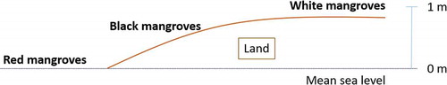
Mangrove occurs in a low salt marsh area with daily intertidal influence (Figure 3). The average elevation for mangrove is between 0 and 1 m above mean sea level (Lopez et al. 2004), and 3 different types of mangrove occur in the Lower Florida Keys: red (Rhizophora mangle), black (Avicennia germinans), and white (Laguncularia racemosa; Monroe County Environmental Education Advisory Council, Inc 1997). Red mangrove occurs in the lowest elevation areas in the coastal area among the 3 mangrove species, with black mangroves at a higher elevation then white mangroves (Figure 4). White mangroves are not as abundant compared to red and black mangroves. White mangroves occur in portions of the coastal area at a relatively higher elevation (N. J. Silvy, unpublished data).

Figure 3. Red mangrove in the Lower Florida Keys (Lopez 2001)

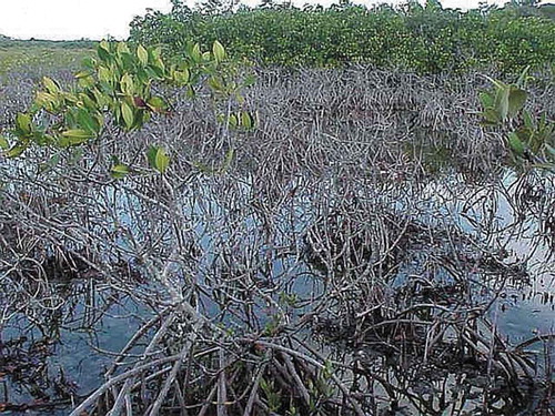
Figure 4. The zonation of 3 different mangroves with respect to elevation

2.2.2. Buttonwoods

Buttonwood (Conocarpus erectus) occurs in a high salt marsh area with infrequent tidal influence (Figure 5). Buttonwood usually occurs between 0.5 and 1 m above mean sea level (Lopez et al. 2004). Saltmeadow cordgrass (Spartina patens) and buttonwood appear in areas higher than mangrove (Monroe County Environmental Education Advisory Council, Inc 1997). Buttonwood appears adjacent to or overlapping with mangrove in a cross section of the vegetation zone, or sometimes appears in the same elevation area (Lopez et al. 2004). Buttonwood is not salt tolerant, and its existence is threatened by rising sea levels (N. J. Silvy, unpublished data).

Figure 5. Buttonwood occurring in the Lower Florida Keys (Lopez 2001)

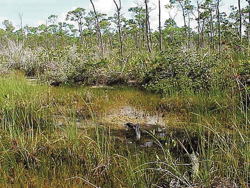
2.2.3. Freshwater marsh

Freshwater marshes are herbaceous and occur between 1 and 2 m above mean sea level (Lopez et al. 2004; Figure 6). Freshwater marsh also can occur in low lying areas in hardwoods/hammocks and pinelands (N. J. Silvy, unpublished data). Freshwater marsh is composed of freshwater holes interspersed with herbaceous plants. Freshwater holes occurring in pinelands and hammocks, which are 2 preferred vegetation types by Key deer, are an important freshwater source for them. In larger freshwater holes on bigger islands, such as the Blue Hole (a gravel pit) on Big Pine Key, a freshwater lens forms on top of sea water, and that is the place where a freshwater marsh can be found (Monroe County Environmental Education Advisory Council, Inc 1997). The fresh water atop the saline water provides a year-round freshwater source for wildlife. Marsh rabbits are usually found in freshwater marshes, especially at higher elevations in grassy areas (saltmeadow cordgrass, Spartina patens) since the vegetation occurring in freshwater marsh provides an excellent food source, shelter, and nesting area for the rabbits (U.S. Fish and Wildlife Service 2019).

Figure 6. Freshwater marsh occurring in the Lower Florida Keys (Lopez 2001)

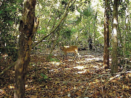
2.2.4. Hardwoods/hammocks

Hammocks refer to a collection of large, mature hardwood trees that occur between 2 and 3 m above mean sea level (Lopez et al. 2004; Figure 7). They are considered to be one of the most unique plant communities occurring in the US (Monroe County Environmental Education Advisory Council, Inc 1997). Most hammocks have mainly open understoreys (N. J. Silvy, unpublished data) and closed canopies, making the understoreys cooler and shadier (Monroe County Environmental Education Advisory Council, Inc 1997). Hardwoods refer to immature hammocks (Silvy 1975), or the precursor of hammocks. Hardwood trees are close to each other and shorter than the larger, taller trees in hammocks (N. J. Silvy, unpublished data). Hardwood trees appear in lower elevation areas than hammocks.

Figure 7. Hammocks occurring in the Lower Florida Keys (Lopez 2001)

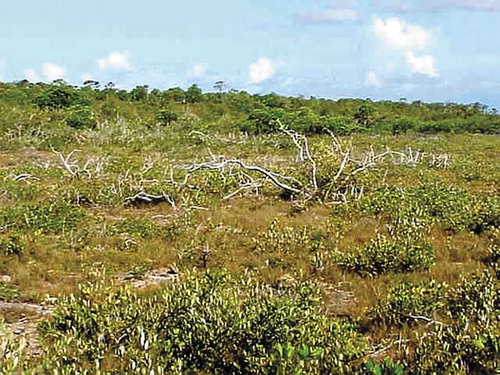
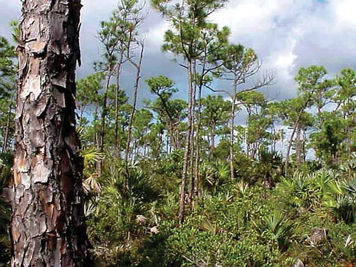
2.2.5. Pineland

Pinelands occur in the highest elevation area in the Keys, with distribution ranges between 2 and 3 m above mean sea level (Lopez et al. 2004; Figure 8). Pinelands have an open, porous canopy (Monroe County Environmental Education Advisory Council, Inc 1997). The openness of the understoreys depends on the occurrence of fire. If there was a recent fire in pinelands, there will be a clear understorey with exposed rocks, dead shrubs, and palms trees displaying only leaves at the tree tops. If there has not been a fire for an extended period of time, there will be a closed-off understorey covered with woody vegetation underneath the pine trees (N. J. Silvy, unpublished data). The pinelands consist of south Florida slash pines (Pinus elliottii var. densa), silver palms (Coccothrinax argentata), thatch palms (Thrinax morrisii), poisonwood (Metopium toxiferum) (Monroe County Environmental Education Advisory Council, Inc 1997) and regeneration of other vegetation from burned pinelands (Silvy 1975). The presence of frequent fires keeps the soil in a state adequate to germinate pine seeds and to keep it from becoming hardwood areas (N. J. Silvy, unpublished data). Along with hammocks, pineland is one of the preferred habitats of Florida Key deer (Lopez et al. 2004) because both hammocks and pineland usually occur in higher elevation areas or upland areas throughout the landscape, and freshwater holes occurring in pinelands provide a freshwater source for Key deer.

Figure 8. Pinelands occurring in the Lower Florida Keys (Lopez 2001)

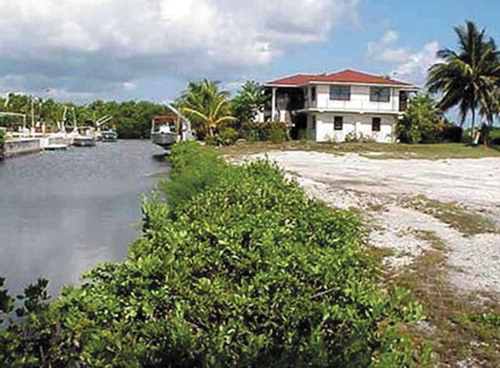
2.2.6. Developed areas

Developed areas usually occur between mangrove and buttonwood (Lopez et al. 2004; Figure 9), since traditionally people wanted to live close to water. The conversion of the low lying areas (where mangroves and buttonwoods used to be) into developed uplands made developed areas more attractive to deer than before. This is because of the higher elevation, and also the presence of ornamental trees inside of the developed areas and surrounding houses, such as rosemallows (Hibiscus spp.), bougainvillea (Bougainvillea glabra), Key lime trees (Citrus aurantiifolia), coconut trees (Cocos nucifera), bracken ferns (Pteridium aquilinum), papayas (Carica spp.), frangipanis (Plumeria spp.), and other plants on which the deer feed (N. J. Silvy, unpublished data).

Figure 9. An example of developed areas in the Lower Florida Keys (Lopez 2001)

2.3. Dataset

Two different sources of input data were employed in the project: 2017 National Agricultural Imagery Program (NAIP) image data and 2008 lidar data. The 2 data sets were the latest publicly available data at the time of data processing. While the NAIP data provided the colour information, the lidar data provided the height and vertical structure information of the vegetation in the study area.

The 2017 NAIP data were downloaded from United States Geological Survey (USGS 2019) Earth Explorer, and the image was acquired on 18 November 2017. The datum of the image was NAD 1983, and the projection was UTM zone 17 N (unit: m). The image had a spatial resolution of 1 × 1 m and had a radiometric resolution of 8 bits. The image had 4 bands (blue, green, red, and near infrared) as the spectral resolution. A band refers to a recorded energy in a specific range of the wavelength (e.g., ultraviolet, visible, and near infrared) of the electromagnetic spectrum (Natural Resources Canada 2019). There were 4 NAIP image tiles for No Name Key, Florida.

The LIght Detection And Ranging (lidar) data were downloaded from the Florida International University (2020) webpage, and the data were collected from 12 January through 8 February 2008. The data were collected from a topographic survey conducted for the State of Florida Division of Emergency Management. The lidar data were in LAS 1.1 file format. There were 8 tiles for No Name Key areas, and the point density for the merged 8 tiles was 2.925 points/m². The lidar data were originally collected in UTM zone 17 N (unit: m) coordinate system, but the data were converted to the Florida State Plane West Zone (unit: feet) after collection and then distributed. The data had NAD83/90 HARN horizontal datum and NAVD88 vertical datum.

In addition to the 2 datasets, a vegetation cover map from a previous vegetation study was employed in this study. Lopez et al. created vegetation cover maps (a shapefile format) of the Lower Florida Keys for the years 1955, 1970, 1985, 2001, and 2015 (Lopez 2001, and TAMU Natural Resource Institute unpublished data). These shapefiles (vector data consisting of points, lines, and polygons) were generated by combining the previous studies, aerial photographs, and land ownership data (Lopez et al. 2004). Among the 5 shapefiles generated from multiple on-going studies, the shapefile from Lopez (2001) was used throughout our study as it was the latest available data at the time the analysis was performed. The shapefile of the vegetation on No Name Key (Lopez 2001) was used for study area extraction and as a reference in collecting training and testing data for producing the updated vegetation map. The visual comparison of the shapefile from 2001 to the one from 2015 revealed that vegetation types have remained fairly consistent over time. The shapefile contained the following 7 different land use/land cover classes: pineland, hammock, freshwater marsh, buttonwood, mangrove, water, and developed. These 7 classes are the classification scheme used in image classifications for our study. The following flowchart (Figure 10) illustrates the processing steps used in this study. For the graphical representation of the input bands used in each of the 2 stacked images (i.e., NAIP stacked image and NAIP-lidar stacked image), refer to Figure 13.

Figure 10. Flowchart of main processing steps used in the study

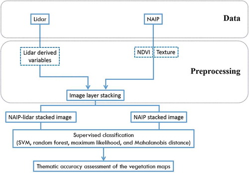
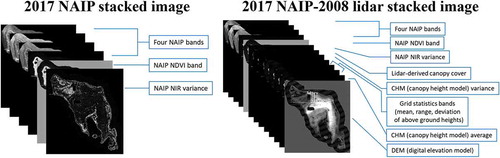
Figure 13. Individual input layers used to create both versions of the stacked image: the 2017 NAIP stacked image and the 2017 NAIP-2008 lidar stacked image (figures were modified from Mutlu et al. (2008))

2.4. Data analysis

2.4.1. NAIP data preprocessing and processing of the NAIP derived layers

Prior to the main processing, we prepared the NAIP data so that it could be used more easily in further data processing. The following 3 steps are the steps that we took to preprocess the NAIP data. The first step in the NAIP data preparation merged all 4 NAIP image tiles for No Name Key area. An image mosaic step was performed in ArcMap^TM software version 10.6.1 (Environmental Systems Research Institute Inc. 2017). In the second step, we converted the coordinate system of the NAIP image (NAD 1983 UTM 17 N) to that of the lidar data (NAD 1983 HARN UTM 17 N).

The third step extracted the study area (i.e., No Name Key area) from the 4 merged tiles. A 250 m buffer around No Name Key area was created from the vegetation shapefile (Lopez 2001) and was used as a clipping template in the study area extraction of the NAIP image. We chose 250 m as the buffer distance to include shoreline and near shore environments. The No Name Key area buffer was also used in extracting the study area for all the layers derived from the NAIP image and lidar data in the later processing steps.

Once the 3 preprocessing steps were completed, the following 2 layers were derived from the NAIP image as a part of the main processing steps: Normalized Difference Vegetation Index (NDVI) band and Variance of Near Infrared (NIR) band. Since the purpose of this study is to classify an image acquired on a single date (rather than to monitor vegetation growth over time or to compare vegetation indices from different dates), we chose not to convert the brightness values (or digital numbers) to reflectance values to calculate NDVI values. Therefore, NDVI was calculated using brightness values of each pixel in band 3 (red) and band 4 (near infrared or NIR) through the following formula:

(1) $\mathrm{N}\mathrm{D}\mathrm{V}\mathrm{I}=\frac{\left(\mathrm{B}{\mathrm{V}}_{\mathrm{N}\mathrm{I}\mathrm{R}}-\mathrm{B}{\mathrm{V}}_{\mathrm{R}\mathrm{e}\mathrm{d}}\right)}{\left(\mathrm{B}{\mathrm{V}}_{\mathrm{N}\mathrm{I}\mathrm{R}}+\mathrm{B}{\mathrm{V}}_{\mathrm{R}\mathrm{e}\mathrm{d}}\right)}$(1)

where BV_NIR indicates the brightness values (or digital numbers) of each pixel in the Near Infrared band (band 4) and BV_Red indicates the brightness values (or digital numbers) of each pixel in the Red band (band 3) in the NAIP image.

The value range for the resulting NDVI layer was from −1 to 1. Areas of barren rock, sand, snow, or ice usually show very low NDVI values (Natural Resources Canada 2019; Campbell and Wynne 2011), for example, 0.1 or less. Sparse vegetation such as shrubs and grasslands or senescing crops may result in moderate NDVI values (Natural Resources Canada 2019), approximately 0.2 to 0.5. There have been numerous studies that have used NDVI to characterize wildlife habitats and their changes, including Hoagland, Beier, and Lee 2018; Hogrefe et al. 2017; St-Louis et al. 2014; Rodgers III, Murrah, and Cooke 2009; Boelman et al. 2016. NDVI was used to measure the amount of green vegetation and the horizontal structure of vegetation (Wood et al. 2012).

Regarding the variance calculations of NIR (band 4), ‘occurrence measures’ in Environment for Visualizing Images (ENVI) software version 5.5.1 (Harris Geospatial Solutions, Inc. 2018) was used with a window size of 3 × 3. Since vegetation reflects near infrared light (Wood et al. 2012), the variance could be used to show the difference in canopy structure or canopy configuration between different vegetation types.

2.4.2. Lidar data preprocessing and processing of the lidar derived layers

The first step in the lidar data preprocessing was to remove obvious error points (or noise) above and below the ground. In removing error points below the ground, any lidar data below −0.61 m (or −2 feet) were removed in relation to the ground elevation and topography of the study site. Rather than using 0 m (or 0 feet) as the threshold, the below-ground error removal threshold of −0.61 m (or −2 feet) was used given that the elevation in some part of No Name Key is below the mean sea level. Moreover, based on trial and error, the threshold of −0.61 m (or −2 feet) resulted in a relatively clean and realistic terrain without removing the actual ground points. For the above-ground error points removal, obvious erroneous points floating above the top of the canopy (which could be from the laser hitting birds or clouds) and laser point hits corresponding to power lines were removed. The noise removal step was performed in Quick Terrain Modeler® (QTM; Applied Imagery 2017) using ‘select polygon (screen)’ tool (for the above-ground error points) and ‘clipping planes’ tool (for the below-ground error points). This noise removal step was performed on each of the 8 tiles individually rather than removing the noise on the combined tiles all at once, since handling each individual tile was easier and quicker to process due to their relatively small size. The second step used the ‘lasmerge’ command in LAStools (rapidlasso GmbH 2014) to merge all 8 noise removed tiles. As the last step in preprocessing, the coordinate system conversion was performed using the ‘las2las’ command in LAStools so that the horizontal and vertical units would be measured in m instead of feet.

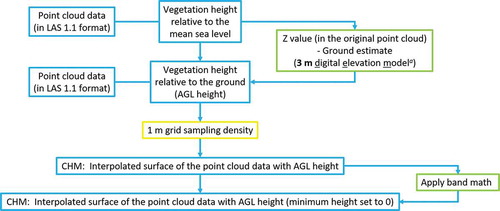
As a part of the processing, 7 layers were derived from the lidar data. They were (1) Percentage Canopy Cover; (2) Variance of Canopy Height Model; (3) Mean, (4) Range, and (5) Deviation of the Above Ground Level (AGL) Height of the laser points; (6) Digital Terrain Model; and (7) Average of Canopy Height Model. Exemplifying these derived layers, the following diagram illustrates the process of creating a Canopy Height Model (CHM) from lidar data (Figure 11).

Figure 11. Flowchart explaining the steps used in the creation of the Canopy Height Model (CHM). ^a 3 m spatial resolution was used in ground estimation by considering the relatively low point density (approximately 2 points per m²) of the lidar data and the flat terrain of the study area

2.4.2.1. Percentage canopy cover

Percentage canopy cover (PCC), which in other studies is equivalent to ‘percent canopy cover’ (PCC; Weishampel et al. (1996), Díaz and Blackburn (2003), Schreuder, Bain, and Czaplewski (2003), Korhonen et al. (2006), Walton, Nowak, and Greenfield (2008), Coulston et al. (2012), McIntosh, Gray, and Garman (2012), Erfanifard, Khodaei, and Shamsi (2014), and Ozdemir (2014)), is a commonly used forestry concept (Erfanifard, Khodaei, and Shamsi 2014) and is important in predicting fire behaviours, air quality and estimating carbon sequestration amounts (Coulston et al. 2012). As discussed in Ozdemir (2014), percentage canopy cover is often used to assess the suitability of wildlife habitat, to manage watershed, and to control erosion. For the rest of the manuscript, we will abbreviate it to PCC to avoid overusing ‘percentage canopy cover’ repeatedly. While (percentage) canopy cover (or PCC) indicates ‘the percentage of a forest area occupied by the vertical projection of tree crowns’ when viewed from above (Purevdorj et al. 1998; Schreuder, Bain, and Czaplewski 2003; Korhonen et al. 2006; Griffin, Popescu, and Zhao 2008; Walton, Nowak, and Greenfield 2008; Paletto and Tosi 2009; McIntosh, Gray, and Garman 2012; Ozdemir 2014), canopy closure refers to ‘the proportion of a hemisphere obscured by vegetation when viewed from a single point’ under the canopy (Paletto and Tosi 2009). Therefore, we computed the PCC with the formula shown below. Our understanding of the PCC is similar to Crookston and Stage (1999), who defined the stand PCC as ‘the percentage of the ground area that is directly covered with tree crowns.’ The PCC layer was estimated by taking the proportion of canopy laser points above a height threshold (e.g., 1 m) out of the total laser points (Lu et al. 2016). Considering the average tree height in the study area, we determined that the threshold of 3 m would result in a good estimation of the canopy cover in the study area. In the study by Grue, Reid, and Silvy (1976), a tree is defined as vegetation taller than 3 m above the ground. Their study analysed and evaluated the breeding habitat of the mourning dove. As such, we adopted a height threshold of 3 m in the calculation of the PCC based on the following formula modified from Griffin (2006):

(2) $\mathrm{P}\mathrm{C}\mathrm{C}=\frac{\mathrm{N}\mathrm{u}\mathrm{m}\mathrm{b}\mathrm{e}\mathrm{r}\mathrm{o}\mathrm{f}\mathrm{t}\mathrm{h}\mathrm{e}\mathrm{a}\mathrm{b}\mathrm{o}\mathrm{v}\mathrm{e}\mathrm{g}\mathrm{r}\mathrm{o}\mathrm{u}\mathrm{n}\mathrm{d}\mathrm{l}\mathrm{a}\mathrm{s}\mathrm{e}\mathrm{r}\mathrm{p}\mathrm{o}\mathrm{i}\mathrm{n}\mathrm{t}\mathrm{s}3\mathrm{m}\mathrm{a}\mathrm{b}\mathrm{o}\mathrm{v}\mathrm{e}\mathrm{g}\mathrm{r}\mathrm{o}\mathrm{u}\mathrm{n}\mathrm{d}\mathrm{w}\mathrm{i}\mathrm{t}\mathrm{h}\mathrm{i}\mathrm{n}\mathrm{a}3\mathrm{m}\mathrm{c}\mathrm{e}\mathrm{l}\mathrm{l}}{\mathrm{T}\mathrm{o}\mathrm{t}\mathrm{a}\mathrm{l}\mathrm{n}\mathrm{u}\mathrm{m}\mathrm{b}\mathrm{e}\mathrm{r}\mathrm{o}\mathrm{f}\mathrm{t}\mathrm{h}\mathrm{e}\mathrm{a}\mathrm{b}\mathrm{o}\mathrm{v}\mathrm{e}\mathrm{g}\mathrm{r}\mathrm{o}\mathrm{u}\mathrm{n}\mathrm{d}\mathrm{l}\mathrm{a}\mathrm{s}\mathrm{e}\mathrm{r}\mathrm{p}\mathrm{o}\mathrm{i}\mathrm{n}\mathrm{t}\mathrm{s}\mathrm{w}\mathrm{i}\mathrm{t}\mathrm{h}\mathrm{i}\mathrm{n}\mathrm{a}3\mathrm{m}\mathrm{c}\mathrm{e}\mathrm{l}\mathrm{l}}$(2)

The choice of a 3 m cell size in calculating the PCC was made considering the lidar point density. The point density of the lidar data used in the project was 2.925 points/m². Considering the relatively low point density of the lidar data, we were hoping to have a sufficient number of points by using a 3 m × 3 m cell size. A 3 m × 3 m cell would result in approximately 27 laser points/9 m², which might be a sufficient number of laser points in calculating a PCC. The 2 layers, the ‘number of the aboveground laser points 3 m above ground within a 3 m cell’ layer and the ‘total number of the aboveground laser points within a 3 m cell’ layer, were created using the ‘Grid Statistics’ in QTM®. The ‘PCC’ layer calculation step itself was performed in ArcToolbox software (Environmental Systems Research Institute Inc. 2017) using the ‘Raster Calculator.’

We used the following 2 steps in creating the Canopy Height Model (CHM) (Figure 11). First, the CHM was initially created by interpolating the laser points with the Above Ground Level (AGL) heights into a smooth surface. In the interpolation, a 1 m × 1 m cell was used as the grid size of the CHM. Second, once the CHM was created, 'band math,' a name for the collection of tools used in processing image bands in ENVI, was applied to the initial CHM to set the negative values (below ground height values of laser points) as 0 m in ENVI (to get the ‘band math' applied 1 m CHM layer).

2.4.2.2. Two derived layers from the CHM

Two additional layers, variance and average of the CHM, were derived from the ‘band math' applied 1 m CHM. The variance of the CHM and the average of the CHM were created by applying a 3 × 3 m filter on the ‘band math' applied 1 m CHM layer. Furthermore, the variance of the CHM was used in processing instead of using the CHM itself because of the variability in the Above Ground Level (AGL) heights. The values of the AGL height variance over trees change frequently while the values of the AGL height variance over houses or other man-made structures do not. In the creation of the CHM variance, we assumed the different crown structure for the tree species present in the study area may result in varying 3D lidar point structure captured by the CHM variance. Similarly, the average of the CHM was used in further processing to see the average tree heights within the given cell size (i.e., a 3 × 3 m cell). Each cell in the ‘CHM average’ layer indicates the average of all the tree height values within each 3 m × 3 m cell size.

2.4.2.3. Mean, range, and deviation of the AGL height data

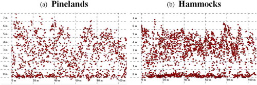
Each of the 3 grid statistics layers (the mean, range, and standard deviation of the above ground level (AGL) height of laser points) was calculated by placing the number of laser points with the AGL heights within a 3 × 3 m grid cell. The Grid Statistics tool in QTM® was used in the calculation of the 3 grid statistics layers. The 2 texture layers (the variance and the average of the CHM) provide information on the tree top (i.e., the top of the Canopy Height Model surface) using a specified filter window size, whereas the result of the Grid Statistics provides information on the vertical structure of the point cloud within a given grid cell size. Figure 12 illustrates examples of vertical profiles of lidar point clouds that depict different point structures of pinelands and hammocks.

Figure 12. Examples of vertical profiles of lidar point clouds that depict different point structures in each area of (a) pinelands vegetation and (b) hammocks vegetation on No Name Key, Florida. The Quick Terrain Modeler^® software was used in the creation of the vertical profiles

2.4.2.4. Digital elevation (or terrain) model

The DEM was created by converting the lowest laser point values (i.e., the ground point) within a 3 m cell into a smooth surface. The topography of the study area is considerably flat, and the elevation of the area is notably low (i.e., 0–3 m above the mean sea level). Since there are 5 distinct vegetation communities in the Lower Florida Keys in such a narrow elevation range, a slight change in the elevation would result in a completely different vegetation type. Therefore, the inclusion of the DEM into the classification process was necessary and important. The reason the 3 m resolution was used in creating the DEM resulted from the consideration of the lidar data point density and the relatively flat terrain of the study area. Given the highest elevation value among the islands in the Lower Florida Keys is less than 3 m (or approximately 8 feet) above the mean sea level (N. J. Silvy and R. R. Lopez, unpublished data; Google Earth Pro software/application 2019), we assumed the elevation did not change much within 9 m² areas. There were negative values in the resulting DEM since some parts of the study area have negative elevation values (i.e., below the mean sea level).

Although the original resolution of some of the lidar derived layers (i.e., percentage canopy cover; mean, range, and deviation of the above ground level height of the laser points; digital terrain model) was 3 m, those layers with a 3 m resolution were resampled into 1 m to match the resolution of the NAIP image and its derived layers (i.e., NAIP NDVI band, NAIP NIR variance). The resampling processes were performed using ArcToolbox software.

2.4.3. Vegetation mapping

2.4.3.1. Normalization

Normalization was performed on the 2 layers derived from the 2017 NAIP image (NDVI and variance of NIR band) and the 7 lidar derived layers using the formula from García et al. (2011). Normalization was applied to avoid inputs in a larger numeric range (e.g., the digital numbers in the NAIP image range from 0 to 255) dominating inputs in a smaller numeric range (e.g., the values in NDVI layer range from −1 to 1; García et al. 2011) while preserving the relative distance from the minimum of each value. The following formula was applied to the following 9 derived bands: the 2 derived bands from the 2017 NAIP image (NDVI band and variance of NIR band) and the 7 derived bands from the lidar point cloud data (PCC; 1 m CHM variance; Mean, Range, and Deviation of laser points with the AGL heights; 1 m CHM average; and 1 m DTM).

(3) $X_{\mathrm{S},i,j}=\frac{Xi,j-X\mathrm{m}\mathrm{i}\mathrm{n}}{X\mathrm{m}\mathrm{a}\mathrm{x}-X\mathrm{m}\mathrm{i}\mathrm{n}}$(3)

where X_i,j indicates an original pixel value (or digital number or brightness value) for each band before scaling is applied at the location i, j (i and j: row and column numbers in each band). X_max represents the maximum value among all the original pixel values within each band. X_min indicates the minimum value among all the original pixel values within each band. Finally, X_S,i,j represents a scaled value for each pixel in each of the 9 derived bands at the location i, j (i and j: row and column numbers in each band).

The formula from García et al. (2011) scaled all the digital numbers so that they were between 0 and 1. The NAIP image is an 8 bit image, and therefore the digital numbers in the NAIP image range between 0 and 255 (i.e., 2⁸ = 256). To match the radiometric resolution of the NAIP image (i.e., 8 bit), the scaled digital numbers, ranging between 0 and 1 (i.e., the result of applying the formula from García et al. (2011)), were multiplied by 255. Each of the 9 derived bands, with the scaling formula applied (the 2 NAIP derived bands and the 7 lidar derived bands), was multiplied by 255. The following is the summary of the normalization formula:

(4) $X_{\mathrm{N},i,j}=X_{\mathrm{S},i,j}\times 255=\left[\frac{Xi,j-X\mathrm{m}\mathrm{i}\mathrm{n}}{X\mathrm{m}\mathrm{a}\mathrm{x}-X\mathrm{m}\mathrm{i}\mathrm{n}}\right]\times 255$(4)

where X_N,i,j represents a normalized value for each pixel in each of the 9 derived bands at the location i, j (i and j: row and column numbers in each band).

Although other normalization formulas exist, the formula from García et al. (2011) was used because it results in more consistent values across different input layers. Considering there was little variation in the minimum of each input band (i.e., X_min) (usually 0 or −1), the numerator (X_i,j – X_min) value was consistent compared to the values generated using a different scaling formula such as $\left[\frac{X\mathrm{m}\mathrm{a}\mathrm{x}-Xi,j}{X\mathrm{m}\mathrm{a}\mathrm{x}-X\mathrm{m}\mathrm{i}\mathrm{n}}\right]$.

The following (Table 1) shows the comparison of the statistics of the values in the original input bands and in the normalized bands in the 2 input images (NAIP stacked and NAIP-lidar stacked images). After the normalization of original bands, the minimum and the maximum values of each original band were adjusted, so that the values of all the normalized bands were approximately within a range between 0 and 255.

Table 1. Comparison of the statistics of the values in the original input bands and in the normalized bands in the 2 input images (2017 NAIP stacked and 2017 NAIP-2008 lidar stacked images). For the description of each band in each of the 2 input images, refer to Table 2

			Minimum	Maximum	Mean	Standard deviation
2017 NAIP stacked image	Original bands	Band 1	0	217	55.753793	53.006792
		Band 2	0	225	61.545515	58.010757
		Band 3	0	224	53.302185	50.263477
		Band 4	0	215	57.752205	75.718131
		Band 5	−0.853333	0.640777	−0.058269	0.333592
		Band 6	0	9067.135742	33.989903	161.325195
	Normalized bands	Band 1	0	217	55.753793	53.006792
		Band 2	0	225	61.545515	58.010757
		Band 3	0	224	53.302185	50.263477
		Band 4	0	215	57.752205	75.718131
		Band 5	−0.000061	254.999939	70.876805	84.799326
		Band 6	0	255	0.955917	4.537036
2017 NAIP-2008 lidar stacked image	Original bands	Band 1	0	217	55.712212	53.008877
		Band 2	0	225	61.499615	58.013455
		Band 3	0	224	53.262432	50.265796
		Band 4	0	215	57.709134	75.706309
		Band 5	−0.853333	0.640777	−0.058226	0.3334710
		Band 6	0	9067.135742	33.964554	161.267696
		Band 7	0	32	0.090205	0.217552
		Band 8	0	2457.617188	0.438046	2.524970
		Band 9	−12.624993	14.850719	0.606783	1.148019
		Band 10	0	159.080002	1.380415	2.521040
		Band 11	0	30.394703	0.433681	0.824503
		Band 12	0	21.937666	0.964876	1.848056
		Band 13	−0.610005	18.529995	−0.018951	0.414399
	Normalized bands	Band 1	0	217	55.733784	53.007320
		Band 2	0	225	61.524337	58.012414
		Band 3	0	224	53.283706	50.264727
		Band 4	0	215	57.726943	75.709847
		Band 5	−0.000061	254.999939	70.846443	84.792150
		Band 6	0	255	0.955553	4.536332
		Band 7	0	255	0.719029	1.733823
		Band 8	0	255	0.045462	0.262019
		Band 9	0	255	70.633649	63.972533
		Band 10	0	255	2.213423	4.041514
		Band 11	0	255	3.639490	6.917922
		Band 12	0	255	11.218263	21.483387
		Band 13	0	255	4.255346	6.706390

2.4.3.2. The creation of 2 input image stacks

After the normalization step, 2 versions of input image stacks (original and normalized) were created for each of the 2 input image sources (NAIP stacked image and NAIP-lidar stacked image). Stacking combined all the separate input layers (or bands) and created 1 single file containing all the different input layers (or bands). The following figure and table (Figure 13 and Table 2) summarize the original input layers used in creating each of the 2 stacked images: the 2017 NAIP stacked image and the 2017 NAIP-2008 lidar stacked image. Table 3 illustrates each of the 2 versions for the 2 input image stacks.

Table 2. The input layers used in the creation of the NAIP stacked image and the NAIP-lidar stacked image

	2017 NAIP stacked image	2017 NAIP-2008 lidar stacked image
Band 1	NAIP Blue band	NAIP Blue band
Band 2	NAIP Green band	NAIP Green band
Band 3	NAIP Red band	NAIP Red band
Band 4	NAIP NIR band	NAIP NIR band
Band 5	NDVI band derived from the 2017 NAIP image	NDVI band derived from the 2017 NAIP image
Band 6	Variance of the 2017 NAIP Near Infrared (NIR) band	Variance of the 2017 NAIP Near Infrared (NIR) band
Band 7		Percentage Canopy Cover
Band 8		Variance of 1 m Canopy Height Model
Band 9		Mean of the Above Ground Level Height of laser points
Band 10		Range of the Above Ground Level Height of laser points
Band 11		Deviation of the Above Ground Level Height of laser points
Band 12		Average of 1 m Canopy Height Model
Band 13		1 m Digital Elevation Model

Table 3. The 2 versions (original and normalized) for each of the 2 input image stacks (NAIP stacked and NAIP-lidar stacked) used in this study

Input image source	NAIP stacked		NAIP-lidar stacked
Input layer (or band) format	Original	Normalized	Original	Normalized

2.4.3.3. Image classification

Image classification or thematic information extraction is a process of converting a raw remotely sensed image into a map with different spectral or information classes without having to digitize it manually. Image classification can be performed either by letting the algorithm break down the input image into spectral clusters without the analyst pre-imposing the classification scheme (thus, unsupervised image classification), or by providing the algorithm with training samples of each of pre-determined information classes (thus, supervised image classification).

Of the 2 types of image classifications (unsupervised and supervised), supervised image classification was performed in this study. The training data for the supervised image classification was collected using the 2017 NAIP-2008 lidar stacked image (not the 2017 NAIP stacked image) on screen and with reference to the 2001 vegetation shapefile and Google Earth® image. One set of the training data collected on the 2017 NAIP-2008 lidar stacked image was used for the classifications of both input sources (the 2017 NAIP stacked image and the 2017 NAIP-2008 lidar stacked image). The vegetation shapefile (Lopez 2001) was used as a vegetation class boundary marker in collecting the training data on-screen. Google Earth^® was used to verify what was seen on our images. We used the 2001 vegetation shapefile, as it was the only available shapefile at the time the training data for each of the 7 classes was collected on-screen.

The following supervised classification algorithms were used to classify each of the 7 land use/land cover types occurring in the study area: machine learning (supervised) methods, such as Support Vector Machine (SVM) and Random Forest, and classical (supervised) methods, such as Maximum Likelihood and Mahalanobis Distance. The SVM, Maximum Likelihood, and Mahalanobis Distance classifications were performed in ENVI software, and the Random Forest classification was performed using R software (R Core Team 2013).

In running the Maximum Likelihood, Mahalanobis Distance, and Random Forest classification algorithms, the default parameters were used in each classification. To restrict the processing area and to reduce the processing time, a classification mask was created using the 250 m buffer shapefile.  The mask was then utilized in performing Maximum Likelihood and Mahalanobis Distance classifications. In performing the Random Forest classification, the code from the Amsantac.co (which code was developed for Landsat 7 images; Santacruz 2019) was used as the starting point, and the code was modified to fit our data. We used the default settings in the following 5 packages in R with no customized values: caret, e1071, raster, rgdal, and snow. The decision to not perform any customization stemmed from the relatively high classification accuracies (compared to other classification algorithms) achieved by the random forest algorithm with the default setting. In addition to performing the image classification, the ‘caret’ package was used to calculate the importance of each of the layers (or variables) in the input images and to plot the importance of them. The variable importance indicates how much each variable (or input layer) contributes in separating each of the land use/land cover classes, with 100 being the most contributing variable and 0 being the least.

For running the SVM classification, the following 2 types of settings were used:  default and custom settings.  In the first setting, the default values were used for all the parameters.  In the custom setting, the values from García et al. (2011) were used for the following 2 parameters:  the penalty parameter (C) and gamma (ɤ).  The default values were used for all other remaining parameters.  As for the custom setting, in addition to using the default values for gamma (ɤ = 1.00) and the penalty parameter (C = 100.00) in the radial basis function kernel type, we adopted the values for the two parameters from García et al. (2011), ɤ = 3.25 and C = 207.94, as a custom setting.  García et al. were able to get the optimal values after conducting a refinement of their grid search result for the two parameters.  Therefore, we considered their search result as the optimal parameters and used them in the classification.  We chose not to perform our own grid search for optimal values for the two parameters because we wanted to get the values from the existing literature rather than running our own search.

2.4.3.4. Post processing

Due to the nature of the high spatial resolution input data (i.e., 1 × 1 m), the classified image resulted in many isolated, small clusters of vegetation cover types. To correct this situation, a 7 × 7 majority filter was applied to each classification output. After each classification was completed, a 7 × 7 majority filter was applied to each classification result, to incorporate the nature of the high spatial resolution data, and to avoid isolated small clusters of cover types with less meaningful ecological interpretation (Chust et al. 2008; Feagin et al. 2010). In applying the majority filter to each of the classification results, all 7 classes, excluding ‘masked pixels’ (only for the classification results of Maximum Likelihood and Mahalanobis Distance) and ‘unclassified,’ were selected using a kernel (or window) size of 7 × 7 and a centre pixel weight of 1. Initially, filter window sizes of 3 × 3, 5 × 5, and 7 × 7 were used in applying the majority filters. A 7 × 7 window resulted in the smoothest and most realistic outcome of applying the filter.

2.4.4. Accuracy assessment

In order to compare the classification results across the input images (NAIP stacked image vs. NAIP-lidar stacked image) and across the input layers format (original vs. normalized), the accuracy of each of the classification output images was assessed in ENVI software using the testing data (i.e., reference data) collected on the 2017 NAIP-2008 lidar stacked image. When the classified image was compared with the reference data, the ‘(overall) classification accuracy’ was estimated by calculating the proportion of correctly classified pixels for each of the land use/land cover classes out of the total pixels in the classified image (Jensen 2015). Along with the (overall) classification accuracy, the к was estimated as a part of the accuracy assessment. The к indicates how much better an image classification is compared to a random-chance assignment of the pixels into each of the land use/land cover classes (Congalton and Green 2009). A confusion matrix (or error matrix; Congalton and Green 2009) was generated as a result of each accuracy assessment. The matrix contained detailed information on each image classification including the correctly classified pixels for each of the land use/land cover classes, the overall accuracy, and the к. The confusion matrix also showed both producer’s accuracy and user’s accuracy for each of the land use/land cover classes. The producer’s accuracy indicates how accurately a producer (or an analyst) produced each of the land use/land cover classes in the map. The user’s accuracy indicates how accurate each land use/land cover class is in terms of a map user’s perspective. In order to reduce bias in assessing the accuracy of the classification results, the training data and the testing data were collected on-screen by 2 separate producers or analysts (i.e., producer 1 and producer 2). In performing the accuracy assessment, the ‘masked pixels’ class (only for the classification results of Maximum Likelihood and Mahalanobis Distance) and the ‘unclassified’ class were excluded. The following formula shows how the (overall) classification accuracy was calculated for each of the classified images. Table 4 summarizes the accuracy assessment scheme used in this study.

(5) $\begin{array}{r}\mathrm{T}\mathrm{h}\mathrm{e}\mathrm{o}\mathrm{v}\mathrm{e}\mathrm{r}\mathrm{a}\mathrm{l}\mathrm{l}\mathrm{c}\mathrm{l}\mathrm{a}\mathrm{s}\mathrm{s}\mathrm{i}\mathrm{f}\mathrm{i}\mathrm{c}\mathrm{a}\mathrm{t}\mathrm{i}\mathrm{o}\mathrm{n}\mathrm{a}\mathrm{c}\mathrm{c}\mathrm{u}\mathrm{r}\mathrm{a}\mathrm{c}\mathrm{y}\\ & =\frac{\begin{array}{c}\mathrm{t}\mathrm{h}\mathrm{e}\mathrm{n}\mathrm{u}\mathrm{m}\mathrm{b}\mathrm{e}\mathrm{r}\mathrm{o}\mathrm{f}\mathrm{c}\mathrm{o}\mathrm{r}\mathrm{r}\mathrm{e}\mathrm{c}\mathrm{t}\mathrm{l}\mathrm{y}\mathrm{c}\mathrm{l}\mathrm{a}\mathrm{s}\mathrm{s}\mathrm{i}\mathrm{f}\mathrm{i}\mathrm{e}\mathrm{d}\mathrm{p}\mathrm{i}\mathrm{x}\mathrm{e}\mathrm{l}\mathrm{s}\\ \mathrm{f}\mathrm{o}\mathrm{r}\mathrm{e}\mathrm{a}\mathrm{c}\mathrm{h}\mathrm{o}\mathrm{f}\mathrm{t}\mathrm{h}\mathrm{e}\mathrm{l}\mathrm{a}\mathrm{n}\mathrm{d}\mathrm{u}\mathrm{s}\mathrm{e}\mathrm{a}\mathrm{n}\mathrm{d}\mathrm{l}\mathrm{a}\mathrm{n}\mathrm{d}\mathrm{c}\mathrm{o}\mathrm{v}\mathrm{e}\mathrm{r}\mathrm{c}\mathrm{l}\mathrm{a}\mathrm{s}\mathrm{s}\mathrm{e}\mathrm{s}\end{array}}{\mathrm{t}\mathrm{h}\mathrm{e}\mathrm{t}\mathrm{o}\mathrm{t}\mathrm{a}\mathrm{l}\mathrm{n}\mathrm{u}\mathrm{m}\mathrm{b}\mathrm{e}\mathrm{r}\mathrm{o}\mathrm{f}\mathrm{p}\mathrm{i}\mathrm{x}\mathrm{e}\mathrm{l}\mathrm{s}\mathrm{i}\mathrm{n}\mathrm{t}\mathrm{h}\mathrm{e}\mathrm{c}\mathrm{l}\mathrm{a}\mathrm{s}\mathrm{s}\mathrm{i}\mathrm{f}\mathrm{i}\mathrm{e}\mathrm{d}\mathrm{i}\mathrm{m}\mathrm{a}\mathrm{g}\mathrm{e}}\end{array}$(5)

Table 4. Depiction of the input using different classification output images in the accuracy assessment step. The accuracy of the total of 40 classified images was evaluated against the reference data collected on the 2017 NAIP-2008 lidar stacked image

		2017 NAIP Stacked				2017 NAIP-2008 lidar stacked
		Original		Normalized		Original		Normalized
SVM		SVM Settings		SVM Settings		SVM Settings		SVM Settings
		Default	Custom	Default	Custom	Default	Custom	Default	Custom
	No filter applied
	Using a 7 × 7 majority filter
Maximum Likelihood	No filter applied
	Using a 7 × 7 majority filter
Mahalanobis Distance	No filter applied
	Using a 7 × 7 majority filter
Random Forest	No filter applied
	Using a 7 × 7 majority filter

3. Results

As a result of implementing the methodology described in the previous section (i.e., the application of the 4 different algorithms on the 2 input sources using different combinations of pre- and post-processing methods), a total of 40 accuracy assessments were performed. The overall result of the accuracy assessment step is summarized in the following. The highest overall classification accuracy and the к were achieved with the Random Forest classification output of the 2017 NAIP-2008 lidar stacked image by using the original input bands and when the 7 × 7 majority filter was applied to the classification output.

The results of the study are graphically represented in the following tables and figures. The results of the accuracy assessment step are summarized in Table 5. Figure 14 is the classified image with the best accuracy across the inputs and the classification algorithms. Table 6 is the confusion matrix of the classified image with the best accuracy out of all the classified images, after the 7 × 7 majority filter was applied. Figure 15 is the classified image with the best accuracy from either version (i.e., original and normalized bands) of the 2017 NAIP stacked images (the original and normalized bands resulted in the same rate of classification accuracy). Figure 16 contains the classified images with the best and the second best accuracies for the 2 versions (i.e., original and normalized bands) of the 2017 NAIP-2008 lidar stacked images. Table 7 is the importance of each layer (or variable) in each of the 4 input images as estimated by the Random Forest algorithm. Figure 17 contains plots that show the importance of each layer (i.e., each variable) in each of the 4 input images as estimated by the Random Forest algorithm.

Figure 14. The classified image of No Name Key, Florida with the best accuracy across the inputs and the classification algorithms. The 7 × 7 majority-filtered classification output from the Random Forest algorithm of the 2017 NAIP-2008 lidar stacked image with the original input bands (not with the normalized bands) achieved both the highest overall classification accuracy and the kappa coefficient (к)

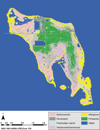
Figure 15. The classified image of No Name Key, Florida with the best accuracy for the 2017 NAIP stacked images. The best classification accuracy for the NAIP stacked image was achieved when using either the original or the normalized bands in the Support Vector Machine (SVM) classification with the new parameter values from García et al. (2011) and applying a 7 × 7 majority filter. The above figure is the SVM classified image of the 7 × 7 majority-filtered 2017 NAIP stacked image with the original bands. It used the new parameter values from García et al. (2011)

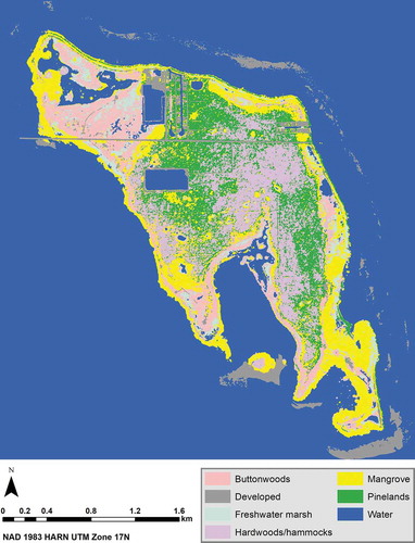
Figure 16. The classified images of No Name Key, Florida with the best and second best accuracies for the 2017 NAIP-2008 lidar stacked images. (a) The best classification accuracy for the NAIP-lidar stacked images was achieved when using the original bands in the Random Forest algorithm and applying a 7 × 7 majority filter. (b) The second best classification accuracy for the NAIP-lidar stacked images was achieved when using the original bands in the Support Vector Machine classification with the new parameter values from García et al. (2011) and applying a 7 × 7 majority filter

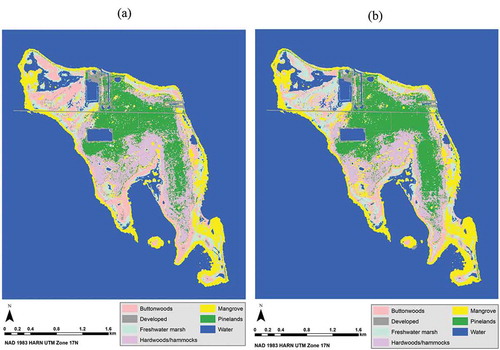
Figure 17. The plots that show the importance of each layer (or variable) in each of the 4 input images as estimated by the Random Forest algorithm. The variable importance of 100 indicates that the variable contributes the most in separating different land use/land cover classes from each other. Similarly, the variable importance of 0 indicates that the variable contributes the least. For the description of each band in each of the 4 input images, refer to either Table 2 or Table 7

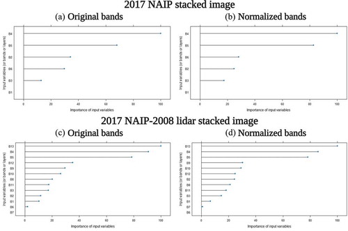
Table 5. Summary of the accuracy assessment results

Classification methods	Post processing	2017 NAIP stacked image				2017 NAIP-2008 lidar stacked image
		Original		Normalized		Original		Normalized
		Default setting	C = 207.94, ɤ = 3.25	Default setting	C = 207.94, ɤ = 3.25	Default setting	C = 207.94, ɤ = 3.25	Default setting	C = 207.94, ɤ = 3.25
Support vector machine	Original output	Overall Accuracy (OA) = 61.1%, kappa coefficient (к) = 0.5467	OA = 62.0%, к = 0.5567	OA = 61.1%, к = 0.5467	OA = 62.0%, к = 0.5567	OA = 71.0%, к = 0.6600	OA = 71.7%, к = 0.6700	OA = 70.3%, к = 0.6533	OA = 72.0%, к = 0.6733
	Applying a 7 × 7 majority filter	OA = 67.4%, к = 0.6200	OA = 68.7%, к = 0.6333	OA = 67.4%, к = 0.6200	OA = 68.7%, к = 0.6333	OA = 70.0%, к = 0.6500	OA = 73.4%, к = 0.6900	OA = 69.4%, к = 0.6433	OA = 70.0%, к = 0.6500
Maximum likelihood	Original output (mask was used in the classification)	OA = 56.7%, к = 0.4933		OA = 56.9%, к = 0.4933		OA = 69.1%, к = 0.6400		OA = 68.7%, к = 0.6333
	Applying a 7 × 7 majority filter	OA = 61.4%, к = 0.5500		OA = 61.4%, к = 0.5500		OA = 72.3%, к = 0.6767		OA = 71.4%, к = 0.6667
Mahalanobis distance	Original output (mask was used in the classification)	OA = 57.4%, к = 0.5033		OA = 57.4%, к = 0.5033		OA = 68.0%, к = 0.6267		OA = 68.6%, к = 0.6333
	Applying a 7 × 7 majority filter	OA = 63.7%, к = 0.5767		OA = 63.7%, к = 0.5767		OA = 71.7%, к = 0.6700		OA = 72.3%, к = 0.6767
Random forest	Original output	OA = 60.7%, к = 0.5412		OA = 59.8%, к = 0.5312		OA = 70.5%, к = 0.6563		OA = 70.6%, к = 0.6567
	Applying a 7 × 7 majority filter	OA = 65.5%, к = 0.5980		OA = 65.3%, к = 0.5947		OA = 75.7%, к = 0.7167		OA = 75.1%, к = 0.7100

Table 6. The confusion matrix generated by comparing the (7 × 7 majority filter-applied) Random Forest algorithm output on the 2017 NAIP-2008 lidar stacked image (with original bands) against the reference data

		Reference data							Total	User’s accuracy (%)	Error of commission (%)
		Ground truth (pixels)
		Water	Pinelands	Mangrove	Hardwoods/hammocks	Freshwater marsh	Developed	Buttonwoods
Random forest classified image	Unclassified	0	0	0	0	0	0	0	0
	Water	139	0	0	0	0	0	0	139	100.00	0.00
	Pinelands	0	130	1	76	0	0	0	207	62.80	37.20
	Mangrove	0	2	112	0	4	0	3	121	92.56	7.44
	Hardwoods/hammocks	0	13	0	74	16	0	0	103	71.84	28.16
	Freshwater marsh	11	5	32	0	78	3	29	158	49.37	50.63
	Developed	0	0	0	0	0	147	3	150	98.00	2.00
	Buttonwoods	0	0	5	0	52	0	115	172	66.86	33.14
	Total	150	150	150	150	150	150	150	1050
Producer’s accuracy (%)		92.67	86.67	74.67	49.33	52.00	98.00	76.67
Error of omission (%)		7.33	13.33	25.33	50.67	48.00	2.00	23.33

^aThe total number of correctly classified pixels = [139 + 130 + 112 + 74 + 78 + 147 + 115] = 795.

^bThe overall classification accuracy (OA) = $\frac{795}{1050}$ = 75.7%

^cKappa coefficient (к) = 0.7167

Table 7. The importance of each layer^a (or variable) in each of the 4 input images as estimated by the Random Forest algorithm, with 100 being the most important and 0 being the least important

2017 NAIP stacked image				2017 NAIP-2008 lidar stacked image
Original bands		Normalized bands		Original bands		Normalized bands
Band 4	100.00	Band 4	100.00	Band 13	100.000	Band 13	100.0000
Band 5	67.96	Band 5	82.65	Band 4	90.807	Band 4	85.8494
Band 2	34.26	Band 6	28.12	Band 5	78.641	Band 5	78.2699
Band 6	29.70	Band 2	24.73	Band 12	35.147	Band 9	30.2770
Band 3	12.78	Band 3	17.53	Band 9	29.524	Band 10	29.0717
Band 1	0.00	Band 1	0.00	Band 10	26.274	Band 12	24.8478
				Band 8	20.047	Band 2	24.2410
				Band 11	17.509	Band 8	21.1122
				Band 3	17.186	Band 11	18.1197
				Band 2	11.612	Band 3	14.6520
				Band 1	10.242	Band 1	6.5382
				Band 6	1.977	Band 7	0.8345
				Band 7	0.000	Band 6	0.0000

^aBand 1: NAIP Blue band, band 2: NAIP Green band, band 3: NAIP Red band, band 4: NAIP Near Infrared (NIR) band, band 5: NDVI band derived from the 2017 NAIP image, band 6: Variance of the 2017 NAIP Near Infrared (NIR) band, band 7: Percentage Canopy Cover, band 8: Variance of 1 m Canopy Height Model, band 9: Mean of the Above Ground Level Height of laser points, band 10: Range of the Above Ground Level Height of laser points, band 11: Deviation of the Above Ground Level Height of laser points, band 12: Average of 1 m Canopy Height Model, band 13: 1 m Digital Elevation Model.

Across all inputs and classification algorithms, the highest overall accuracy and к were achieved by the Random Forest classification on the 2017 NAIP-2008 lidar stacked image with an applied 7 × 7 majority filter, and original input bands (Figure 14). In comparison to the classification accuracies between classification results of the 2017 NAIP stacked image and classification results of the 2017 NAIP-2008 lidar stacked image, the accuracies of the classification results from the 2017 NAIP-2008 lidar stacked images were always higher than the accuracies of the 2017 NAIP stacked images.

In order to explore the impact of normalization on the classification accuracy, the accuracy of the classification outputs from the original layers (or bands) was compared with the accuracy of the classification outputs from the normalized layers (or bands). There were only small differences in accuracy between the 2 input band types (the original and the normalized bands). In fact, for 3 of the classification results of the 2017 NAIP stacked images (SVM, Maximum Likelihood, and Mahalanobis Distance), there was no improvement in accuracy in reference to normalized bands. For the Random Forest classification of the 2017 NAIP stacked images, normalization slightly lowered the classification accuracies. For the classification results of the 2017 NAIP-2008 lidar stacked images, 60% of the time, the results using the normalized bands were less accurate than the original bands.

To examine the impact of the majority filter application on the classification accuracy, the accuracies of the original classification and the majority filtered classification results were compared. In most cases, the accuracies of the majority filter-applied classification results were higher than the actual classification results across the input sources (NAIP alone or NAIP combined with lidar), across the settings used in the classification (default setting vs. some other values used for the classification parameters), across the classification algorithms used (SVM, Maximum Likelihood, Mahalanobis, or Random Forest), and regardless of the normalization (original bands vs. normalized bands). Findings for each of the 4 algorithms are discussed below.

3.1. SVM algorithm

The classification using the SVM algorithm on the 2017 NAIP-2008 lidar stacked images with the majority filter applied, as well as the new parameter values (from García et al. 2011), produced the highest accuracy (overall accuracy: 73.4% and the к: 0.6900). For the SVM classification results of the 2017 NAIP stacked images, applying the majority filter increased the classification accuracy, and there was no difference in the accuracy of the classification results when the original and the normalized bands were used (Figure 15). For the SVM classification results of the 2017 NAIP-2008 lidar stacked images, 75% of the time applying the majority filter actually lowered the classification accuracy, and the normalization did not seem to increase the accuracy of the classification results. García et al. (2011) showed a slight increase in the accuracies of the SVM classified images when using the new optimal parameter values for the penalty parameter (C) and the gamma (ɤ) in comparison to using the default values for the 2 parameters. Our results were consistent with García et al.’s findings.

3.2. Maximum likelihood algorithm

The classification using the Maximum Likelihood algorithm on the 2017 NAIP-2008 lidar stacked image with the majority filter applied and using the original bands produced the highest accuracy (overall accuracy: 72.3% and the к: 0.6767). For the Maximum Likelihood classification results of the 2017 NAIP stacked images, applying the majority filter increased the classification accuracy, and the normalization did not affect the accuracy of the classification results. For the Maximum Likelihood classification results of the 2017 NAIP-2008 lidar stacked images, applying the majority filter increased the classification accuracy, and the normalization slightly lowered the accuracy of the classification results.

3.3. Mahalanobis distance algorithm

The classification using the Mahalanobis Distance algorithm on the 2017 NAIP-2008 lidar stacked image with the majority filter applied and using the normalized bands produced the highest accuracy (overall accuracy: 72.3% and the к: 0.6767). For the Mahalanobis classification results of the 2017 NAIP stacked images, applying the majority filter slightly increased the classification accuracy, and the normalization did not increase the accuracy of the classification results at all. For the Mahalanobis Distance classification results of the 2017 NAIP-2008 lidar stacked images, applying the majority filter increased the classification accuracy, and the normalization helped improving the accuracy of the classification results marginally.

3.4. Random forest algorithm

The classification using the Random Forest algorithm on the 2017 NAIP-2008 lidar stacked image with the majority filter applied and using the original bands produced the highest accuracy (Figure 14; overall accuracy: 75.7% and the к: 0.7153). For the Random Forest classification results of the 2017 NAIP stacked images, applying the majority filter increased the classification accuracy, and the normalization slightly lowered the accuracy of the classification results. For the Random Forest classification results of the 2017 NAIP-2008 lidar stacked images, applying the majority filter increased the classification accuracy, and the normalization did not make a significant difference in the accuracy of the classification results.

The following comparisons were made for each of the 4 classification algorithms to determine which combination of the pre- and post- processing methods increased the classification accuracy and to show which input image source resulted in a higher classification accuracy. When the comparison of classification accuracies was made across the input sources for each classification algorithm (using the default setting) with and without the application of the 7 × 7 majority filter, the classification accuracy of the Support Vector Machine method was the highest for the 2017 NAIP-2008 lidar stacked image with the original bands and without the application of the 7 × 7 majority filter. The classification accuracy of the Maximum Likelihood method was the highest for the 2017 NAIP-2008 lidar stacked image with the original bands and with the 7 × 7 majority filter applied. The classification accuracy of the Mahalanobis Distance method was the highest for the 2017 NAIP-2008 lidar stacked image with the normalized bands and with the majority filter applied. Finally, the classification accuracy of the Random Forest method was the highest for the 2017 NAIP-2008 lidar stacked image with the original bands and with the 7 × 7 majority filter applied.

4. Discussion and conclusions

4.1. Discussion

In terms of the input data sources, the classification accuracies of the NAIP-lidar stacked images were higher than the accuracies of the NAIP stacked images. It was true for the following conditions: (1) no matter which classification algorithm (SVM, Maximum Likelihood, Mahalanobis Distance, or Random Forest) we used, (2) whether we applied the post classification processing method (i.e., applying the majority filter once for each classification), (3) whether we used the original bands or the normalized bands in the classification of both the NAIP stacked images and the NAIP-lidar stacked images, and (4) regardless of the settings we used in the SVM classification (default or custom settings).

In analysing the accuracy assessment results, the confusion matrix of the classification result with the highest classification accuracy (i.e., the 7 × 7 majority filter-applied, Random Forest algorithm output on the 2017 NAIP-2008 lidar stacked image with the original bands; Table 6) showed the following. The water class had the highest producer’s and user’s accuracies, the hardwoods/hammocks class had the lowest producer’s accuracy, and the freshwater marsh class had the lowest user’s accuracy. There was confusion between the following class pairs: mangrove and freshwater marsh classes, pinelands and hardwoods/hammocks classes, water and freshwater marsh classes, freshwater marsh and buttonwoods classes, and freshwater marsh and hardwoods/hammocks classes.

In comparison of the classification accuracies between the 2 input data sources, adding the lidar data to the multispectral data improved the accuracy of vegetation maps, as expected. A possible reason the NAIP-lidar stacked image yielded a higher classification accuracy might be that the lidar data provides information on the vertical distribution of the vegetation in the study area, which the optical data alone cannot provide. This matches the findings from Mutlu, Popescu, and Zhao (2008).

Regarding classification algorithms, the machine learning algorithms produced a higher rate of accuracy compared to the classification results using the classical algorithms. The Random Forest algorithm produced the highest rate of accuracy among the 4 algorithms. One of the advantages of using the Random Forest algorithm is that the algorithm provides the importance or rank of all the variables (or input layers) in each input image (Table 7 and Figure 17). The variable importance indicates the contribution of each variable (or band) in the Random Forest classification process; the higher the variable importance is, the more contribution the variable (or band) makes in separating different land use/land cover classes. The variable importance for the 2017 NAIP stacked images showed the following: in both versions of the 2017 NAIP stacked image (original and normalized versions), the near infrared band (band 4) was the most important, followed by the NDVI band (band 5). The blue band (band 1) was least important in separating different classes in the 2 versions of the 2017 NAIP input images. In both versions of the 2017 NAIP-2008 lidar stacked image (whether the bands were normalized or not), the Digital Elevation Model (band 13) was the most important, followed by the near infrared band (band 4), and the NDVI band (band 5). The DEM band (band 13) may be the most important variable in the Random Forest classification because of the importance of elevation in determining the zonation of the coastal vegetation. However, band 7 (percentage canopy cover) was least important in the original version, and band 6 (variance of the near infrared band) was least important in the normalized version of the 2017 NAIP-2008 lidar stacked images. In most cases, lidar-derived variables (or bands) proved to be important in separating different land use/land cover classes.

In terms of pre-processing, when the accuracy of the classification outputs using the normalized bands in the 2017 NAIP-2008 lidar stacked images was examined, it was clear that in most cases the normalization did not improve the classification accuracy. Normalization was meant to prevent values with a larger numeric value range from impacting values in an input band with a smaller numeric range (García et al. 2011). As a result of the normalization process, the data ranges for different bands coming from different sources were all set to the same numeric range.

Regarding post-classification processing, the application of the majority filter increased the accuracy of the classification results, as expected. In most cases, the accuracies of the majority filter-applied classification results were higher than the actual classification results. This was true across the input sources, the classification settings, and the classification algorithms, regardless of the normalization. One explanation for this might be that the testing data (or reference data) are point data, not polygons. Additionally, the classification does not always produce a homogeneous patch consisting of the same vegetation type pixels, meaning only 1 class of vegetation pixels. The classification often results in a mosaic of different vegetation class pixels. Due to these 2 reasons, it is more likely that the testing data (or reference data) can fall on the surrounding areas of a different vegetation class (not the same vegetation class as that of the testing data pixel), and lower the accuracy assessment results.

Additionally, the classification accuracy could be affected by the classification training data separability between any 2 different classes. Once the training data collection was completed, the separability of the training data for both stacked images was examined. The following classes showed poor separability, which could contribute to the low classification accuracies: mangroves and hardwoods/hammocks, mangroves and pinelands, and pinelands and hardwoods/hammocks. By improving the separability of these class pairs with more accurate training data collection, better classification results can be achieved.

The absence of ground truth data could have contributed to the classification accuracy. As previously mentioned, the shapefile from Lopez (2001) was used as each vegetation class boundary in collecting both the training and testing (or reference) data on-screen, in the absence of ground truth data. The classification results could be biased since we used the existing vegetation shapefile (Lopez 2001) as a vegetation class boundary marker rather than using the data collected in the field. Using the GPS data collected in the study area as the training and testing data (rather than solely using the information from the existing shapefile) or collecting data on-screen without using the information from the shapefile could have resulted in a more unbiased and accurate classification.

Exploring more ways to create different combinations of input data sources could lead to improved classification results. For the texture bands of the lidar data (e.g., 3 × 3 m variance of the CHM), only 2 textures, variance and mean, were considered. Furthermore, only 1 processing window or filter size (i.e., 3 × 3 m) was used. Exploring all the combinations of different textures (such as data range, entropy, and skewness) and different window sizes (such as 5 × 5, 7 × 7, 9 × 9, etc.) would result in more accurate vegetation maps.

Moreover, the difference in the data collection timeframe would need to be acknowledged when assessing the classification accuracy. While the NAIP image was acquired in 2017, the lidar data was collected in 2008. The 9 year time discrepancy between the 2 datasets could have resulted in a lower classification accuracy. We certainly need to consider vegetation growth and hurricanes between 2008 and 2017 in interpreting the classification results. The impact of storms on ecosystems includes changes in vegetation communities, such as wind-thrown trees, broken branches, or defoliation, and includes decreases in freshwater availability (Lopez 2001). Two storms/hurricanes (i.e., Tropical Storm Fay (August 2008) and category 4 Hurricane Irma (September 2017)) passed through the Florida Keys between 2008 and 2017 (National Oceanic and Atmospheric Administration [NOAA] 2019). We assumed that it would be acceptable to use the lidar data from 2008 due to the following reasons. First, lidar should be able to pick up the structural differences between different vegetation types. Second, the topography itself might not change much between different years. When the topography changes little, upland vs. low-land area remains the same. With this rationale, we hoped that the lidar data would be able to detect structural attributes of different vegetation types.

In terms of lidar height data, a number of studies report that the measurements taken from laser instruments in aircrafts underestimate the vegetation heights (Lim et al. 2003; Srinivasan et al. 2014). Therefore, we need to account for these potential deviations by incorporating lidar height measurements acquired by using a terrestrial laser scanner or derived from the Structure from Motion (SfM) technique.

Note that the developed areas are not entirely made up of buildings or houses. There is also some vegetation near/around residential or developed areas. Among these areas are ornamental trees such as rosemallows, bougainvillea, coconut trees, papayas, bracken ferns, Key lime trees, and frangipanis (N. J. Silvy, unpublished data). It would be better to digitally delineate the vegetation inside of the developed areas and surrounding houses in the input images. Excluding the delineated area in the image classifications could result in a more accurate depiction of the wildlife habitat in the study area.

Regarding land management, it is important to understand the effect of the lack of prescribed burning on pinelands. Fire keeps pinelands from transitioning into hardwood trees and also prevents hardwood trees from becoming hammocks. To maintain the pinelands vegetation areas, regular prescribed burning (e.g., every 3–5 years) is essential to help regeneration by burning dead pines and clearing the soil (Lopez et al. 2004). Due to the absence of prescribed burning in the Lower Keys, hardwood trees have replaced some pineland areas (N. J. Silvy, unpublished data). The pinelands are important in terms of their unique structure, an open, porous pine canopy structure and understorey cover composed of shrubs, grasses, and herbs (Lopez et al. 2004). Regular prescribed burning is necessary and beneficial to maintain the biodiversity of plant and wildlife communities.

4.2. Conclusions

It is important to have accurate land use/land cover maps in wildlife and natural resource management because they help wildlife and natural resource managers effectively maintain natural resources. Other studies emphasized the importance of long term monitoring and management of endangered species habitats because suitable habitats will ensure the future survival of native wildlife, such as Key deer (Silvy 1975; Lopez 2001). Considering the devastating effect of Hurricane Irma on the Florida Keys (especially on Big Pine Key and surrounding islands), we can act on this need to monitor wildlife by creating more accurate vegetation maps (airborne data combined with lidar data) to use as inputs for the spectral change detection analysis of vegetation before and after Hurricane Irma. The results from this study, combined with the existing land use/land cover maps of the study area, will enhance the effectiveness of managing natural resources including the endangered wildlife species of the region. The results will also help improve the conservation of species including Lower Keys marsh rabbits. The methodology used in our study could be applied to studies for other islands in the Lower Florida Keys or similar environmental conditions.

The study has several findings. First, the structural information from lidar data enhanced the information from aerial images. The classified map of airborne data combined with lidar data resulted in a higher classification accuracy in vegetation mapping on No Name Key compared to the airborne data alone. Second, when normalization was applied to all the input bands or layers, the classification accuracies were not increased in most cases. Third, new machine learning algorithms worked better in characterizing habitats, compared to other classical algorithms. The classified map produced with the Random Forest algorithm with the original (i.e., non-normalized) bands resulted in the highest classification accuracy. Fourth, in most cases, the application of the majority filter (using a 7 × 7 window size) increased the accuracy of the classification results compared to the classification results when no majority filter was applied. Lastly, instead of using the default values, when the new parameter values (from García et al. 2011) for the penalty parameter (C) and the gamma (ɤ) were used, the accuracies of the SVM classified images were slightly increased compared to using the default values for the 2 parameters.

This study suggested that we can successfully map post hurricane vegetation with sufficient accuracy. The availability of public lidar data has greatly increased, especially with the launch of the ICESat II satellite (Popescu et al. 2018). This increased availability allows researchers to obtain more accurate vegetation information in their study areas, particularly after major storms and hurricanes. Rather than using multispectral images alone, the fusion of lidar and aerial/satellite data (i.e., multispectral images) provides an improved method of creating habitat maps. Vegetation studies using lidar data combined with airborne or spaceborne images would enhance the accuracy of vegetation mapping. When creating maps of land cover types using the combined input images with the method described in this study, considering the small difference in accuracy between the Random Forest and SVM classified images, either the Random Forest or the SVM algorithm would be a good starting point. The choice between the 2 algorithms could be decided according to the preference of the researcher. In applying either the SVM or the Random Forest algorithm, normalization of the original input bands may not be necessary, use of the default settings may not guarantee the highest classification accuracy (for the SVM algorithm), and the application of a majority filter would be appropriate, especially in vegetation mapping studies for habitat characterization.

Acknowledgements

We would like to thank L. Malambo and R. Feagin for their help in this study. We also would like to thank the anonymous reviewers for their insightful comments on this manuscript. M. Andrews, the technical editor, has offered guidance throughout the technical editing process. We are thankful for his help and patience. Our special thanks goes to everyone at Texas A&M University Writing Centre for their tremendous help throughout the entire writing process—their support and feedback from the initial drafting stage to the final revision phase have been an invaluable and integral part of the manuscript. J. K. would especially like to thank Youhee and Jinghyun Kim for their continuous support, encouragement, and guidance.

Disclosure statement

No potential conflict of interest was reported by the authors.

References

- Applied Imagery. 2017. Quick Terrain Modeler (QTM) Software (Version 8.0.7.1). Chevy Chase, Maryland, USA.
- Bergen, K. M., S. J. Goetz, R. O. Dubayah, G. M. Henebry, C. T. Hunsaker, M. L. Imhoff, R. F. Nelson, G. G. Parker, and V. C. Radeloff. 2009. “Remote Sensing of Vegetation 3‐D Structure for Biodiversity and Habitat: Review and Implications for LiDaR and Radar Spaceborne Missions.” Journal of Geophysical Research 114 (G2): 1–13. doi:10.1029/2008JG000883.
- Boelman, N. T., J. D. Holbrook, H. E. Greaves, J. S. Krause, H. E. Chmura, T. S. Magney, J. H. Perez, J. U. H. Eitel, L. Gough, K. T. Vierling, J. C. Wingfield, and L. A. Vierling. 2016. “Airborne Laser Scanning and Spectral Remote Sensing Give a Bird’s Eye Perspective on Arctic Tundra Breeding Habitat at Multiple Spatial Scales.” Remote Sensing of Environment 184: 337–349. doi:10.1016/j.rse.2016.07.012.
- Bouchhima, R. A., M. Sarti, M. Ciolfi, M. Lauteri, and M. Ksibi. 2018. “Decision Tree for Mapping of Halophyte Cover around Ghannouch, Tunisia.” Environmental Monitoring and Assessment 192 (12): 742. doi:10.1016/j.rse.2016.07.012.
- Campbell, J. B., and R. H. Wynne. 2011. Introduction to Remote Sensing. 5th ed. New York: Guilford Press.
- Chust, G., I. Galparsoro, Á. Borja, J. Franco, and A. Uriarte. 2008. “Coastal and Estuarine Habitat Mapping, Using LIDAR Height and Intensity and Multi-spectral Imagery.” Estuarine, Coastal and Shelf Science 78 (4): 633–643. doi:10.1016/j.ecss.2008.02.003.
- Congalton, R. G., and K. Green. 2009. Assessing the Accuracy of Remotely Sensed Data: Principles and Practices. Boca Raton: CRC Press.
- Coulston, J. W., G. G. Moisen, B. T. Wilson, M. V. Finco, W. B. Cohen, and C. K. Brewer. 2012. “Modeling Percent Tree Canopy Cover: A Pilot Study.” Photogrammetric Engineering & Remote Sensing 78 (7): 715–727. doi:10.14358/PERS.78.7.715.
- Crookston, N. L., and A. R. Stage. 1999. Percent Canopy Cover and Stand Structure Statistics from the Forest Vegetation Simulator. General Technical Report RMRS-GTR-24, 11. Ogden, UT:United States Department of Agriculture, Forest Service, Rocky Mountain Research Station. doi:10.2737/RMRS-GTR-24.
- Díaz, B. M., and G. A. Blackburn. 2003. “Remote Sensing of Mangrove Biophysical Properties: Evidence from a Laboratory Simulation of the Possible Effects of Background Variation on Spectral Vegetation Indices.” International Journal of Remote Sensing 24 (1): 53–73. doi:10.1080/01431160305012.
- Environmental Systems Research Institute Inc. 2017. ArcMap™ Desktop Software (Version 10.6.1.9270). Redlands, California, USA.
- Erfanifard, Y., Z. Khodaei, and R. F. Shamsi. 2014. “A Robust Approach to Generate Canopy Cover Maps Using UltraCam-D Derived Orthoimagery Classified by Support Vector Machines in Zagros Woodlands, West Iran.” European Journal of Remote Sensing 47 (1): 773–792. doi:10.5721/EuJRS20144744.
- Faulhaber, C. A. 2003. “Updated distribution and reintroduction of the Lower Keys marsh rabbit.” PhD diss., Texas A&M University, College Station, TX, USA. http://hdl.handle.net/1969.1/1348
- Feagin, R. A., M. L. Martinez, G. Mendoza-Gonzalez, and R. Costanza. 2010. “Salt Marsh Zonal Migration and Ecosystem Service Change in Response to Global Sea Level Rise: A Case Study from an Urban Region.” Ecology and Society 15 (4): 14. doi:10.5751/ES-03724-150414.
- Florida International University. 2020. “Lidar (Light Detection and Ranging) Data.” Accessed 17 January 2020. http://digir.fiu.edu/Lidar/lidarNew.php
- García, M., D. Riaño, E. Chuvieco, J. Salas, and F. M. Danson. 2011. “Multispectral and LiDAR Data Fusion for Fuel Type Mapping Using Support Vector Machine and Decision Rules.” Remote Sensing of Environment 115 (6): 1369–1379. doi:10.1016/j.rse.2011.01.017.
- Gislason, P. O., J. A. Benediktsson, and J. R. Sveinsson. 2006. “Random Forests for Land Cover Classification.” Pattern Recognition Letters 27 (4): 294–300. doi:10.1016/j.patrec.2005.08.011.
- Google Earth Pro software/application. 2019. Google LLC, Mountain View,California, USA.
- Griffin, A. M. R. 2006. “Using Lidar and Normalized Difference Vegetation Index to Remotely Determine LAI and Percent Cover at Varying Scales.” Thesis, Texas A&M University, College Station. http://hdl.handle.net/1969.1/ETD-TAMU-1117
- Griffin, A. M. R., S. C. Popescu, and K. Zhao. 2008. “Using LIDAR and Normalized Difference Vegetation Index to Remotely Determine LAI and Percent Canopy Cover.” In Proceedings of SilviLaser 2008: 8th international conference on LiDAR applications in forest assessment and inventory, Edinburgh, UK. September 17–19, pp 446–455. https://geography.swan.ac.uk/silvilaser/papers/poster_papers/Griffin.pdf
- Grue, C. E., R. R. Reid, and N. J. Silvy. 1976. “A Technique for Evaluating the Breeding Habitat of Mourning Doves Using Call-count Transects.” Proceeding of the Annual Conference of the Southeastern Association of Game and Fish Commissioners 30: 667–673.
- Haest, B., J. V. Borre, T. Spanhove, G. Thoonen, S. Delalieux, L. Kooistra, C. A. Mücher, D. Paelinckx, P. Scheunders, and P. Kempeneers. 2017. “Habitat Mapping and Quality Assessment of NATURA 2000 Heathland Using Airborne Imaging Spectroscopy.” Remote Sensing 9 (3): 266. doi:10.3390/rs9030266.
- Harris Geospatial Solutions, Inc. 2018. Environment for Visualizing Images (ENVI) Software (Version 5.5.1). Boulder, Colorado, USA.
- Harveson, P. M., W. E. Grant, R. R. Lopez, N. J. Silvy, and P. H. Frank. 2006. “The Role of Dispersal in Florida Key Deer Metapopulation Dynamics.” Ecological Modelling 195 (3–4): 393–491. doi:10.1016/j.ecolmodel.2005.11.021.
- Hoagland, S., P. Beier, and D. Lee. 2018. “Using MODIS NDVI Phenoclasses and Phenoclusters to Characterize Wildlife Habitat: Mexican Spotted Owl as a Case Study.” Forest Ecology and Management 412: 80–93. doi:10.1016/j.foreco.2017.12.017.
- Hogrefe, K., V. Patil, D. Ruthrauff, B. Meixell, M. Budde, J. Hupp, and D. Ward. 2017. “Normalized Difference Vegetation Index as an Estimator for Abundance and Quality of Avian Herbivore Forage in Artic Alaska.” Remote Sensing 9 (12): 1234. doi:10.3390/rs9121234.
- Huang, C., L. S. Davis, and J. R. G. Townshend. 2002. “An Assessment of Support Vector Machines for Land Cover Classification.” International Journal of Remote Sensing 23 (4): 725–749. doi:10.1080/01431160110040323.
- Jensen, J. R. 2015. Introductory Digital Image Processing: A Remote Sensing Perspective. 4th ed. Prentice Hall, Upper Saddle River, New Jersey, USA.
- Korhonen, L., K. T. Korhonen, M. Rautiainen, and P. Stenberg. 2006. “Estimation of Forest Canopy Cover: A Comparison of Field Measurement Techniques.” Silva Fennica 40 (4): 577–588. doi:10.14214/sf.315.
- LaFever, D. H., R. R. Lopez, R. A. Feagin, and N. J. Silvy. 2007. “Predicting the Impacts of Future Sea-level Rise on an Endangered Lagomorph.” Environmental Management 40 (3): 430–437. doi:10.1007/s00267-006-0204-z.
- Lim, K., P. Treitz, M. Wulder, B. St-Onge, and M. Flood. 2003. “LiDAR Remote Sensing of Forest Structure.” Progress in Physical Geography: Earth and Environment 27 (1): 88–106. doi:10.1191/0309133303pp360ra.
- Lopez, R. R. 2001. “Population Ecology of Florida Key Deer.” Dissertation, Texas A&M University, College Station, Texas, USA. http://proxy.library.tamu.edu/login?url=https://search.proquest.com/docview/276225755?accountid=7082
- Lopez, R. R., N. J. Silvy, R. N. Wilkins, P. A. Frank, M. J. Peterson, and M. N. Peterson. 2004. “Habitat-use Patterns of Florida Key Deer: Implications of Urban Development.” Journal of Wildlife Management 68 (4): 900–908. doi:10.2193/0022-541X(2004)068[0900:HPOFKD]2.0.CO;2.
- Lu, D., Q. Chen, G. Wang, L. Liu, G. Li, and E. Moran. 2016. “A Survey of Remote Sensing-based Aboveground Biomass Estimation Methods in Forest Ecosystems.” International Journal of Digital Earth 9 (1): 63–105. doi:10.1080/17538947.2014.990526.
- Martínez, M. L., A. Intralawan, G. Vázquez, O. Pérez-Maqueo, P. Sutton, and R. Landgrave. 2007. “The Coasts of Our World: Ecological, Economic and Social Importance.” Ecological Economics 63 (2–3): 254–272. doi:10.1016/j.ecolecon.2006.10.022.
- McIntosh, A. C. S., A. N. Gray, and S. L. Garman. 2012. “Estimating Canopy Cover from Standard Forest Inventory Measurements in Western Oregon.” Forest Science 58 (2): 154–167. doi:10.5849/forsci.09-127.
- Monroe County Environmental Education Advisory Council, Inc. 1997. “The Florida Keys Environmental Story.” D. Gallagher, editor. Monroe County Environmental Education Advisory Council, Inc., Big Pine Key, Florida, USA.
- Mountrakis, G., J. Im, and C. Ogole. 2011. “Support Vector Machines in Remote Sensing: A Review.” International Society for Photogrammetry and Remote Sensing Journal of Photogrammetry and Remote Sensing 66 (3): 247–259. doi:10.1016/j.isprsjprs.2010.11.001.
- Mutlu, M., S. C. Popescu, and K. Zhao. 2008. “Sensitivity Analysis of Fire Behavior Modeling with LIDAR-derived Surface Fuel Maps.” Forest Ecology and Management 256 (3): 289–294. doi:10.1016/j.foreco.2008.04.014.
- Na, X., S. Zhang, X. Li, H. Yu, and C. Liu. 2010. “Improved Land Cover Mapping Using Random Forests Combined with Landsat Thematic Mapper Imagery and Ancillary Geographic Data.” Photogrammetric Engineering & Remote Sensing 76 (7): 833–840. doi:10.14358/PERS.76.7.833.
- National Oceanic and Atmospheric Administration [NOAA]. 2019. “Historical Hurricane Tracks Data.” https://coast.noaa.gov/hurricanes
- Natural Resources Canada. 2019. “The Canada Centre for Mapping and Earth Observation: Fundamentals of Remote Sensing.” https://www.nrcan.gc.ca/sites/www.nrcan.gc.ca/files/earthsciences/pdf/resource/tutor/fundam/pdf/fundamentals_e.pdf
- Ozdemir, I. 2014. “Linear Transformation to Minimize the Effects of Variability in Understory to Estimate Percent Tree Canopy Cover Using RapidEye Data.” GIScience & Remote Sensing 51 (3): 288–300. doi:10.1080/15481603.2014.912876.
- Paletto, A., and V. Tosi. 2009. “Forest Canopy Cover and Canopy Closure: Comparison of Assessment Techniques.” European Journal of Forest Research 128 (3): 265–272. doi:10.1007/s10342-009-0262-x.
- Popescu, S. C., T. Zhou, R. Nelson, A. Neuenschwander, R. Sheridan, L. Narine, and K. M. Walsh. 2018. “Photon Counting LiDAR: An Adaptive Ground and Canopy Height Retrieval Algorithm for ICESat-2 Data.” Remote Sensing of the Environment 208: 154–170. doi:10.1016/j.rse.2018.02.019.
- Purevdorj, Ts., R. Tateishi, T. Ishiyama, and Y. Honda. 1998. “Relationships between Percent Vegetation Cover and Vegetation Indices.” International Journal of Remote Sensing 19 (18): 3519–3535. doi:10.1080/014311698213795.
- Putman, E. B., and S. C. Popescu. 2018. “Automated Estimation of Standing Dead Tree Volume Using Voxelized Terrestrial Lidar Data.” IEEE Transactions on Geoscience and Remote Sensing 56 (11): 6484–6503. doi:10.1109/TGRS.2018.2839088.
- R Core Team. 2013. R: A Language and Environment for Statistical Computing. R Foundation for Statistical Computing, Vienna, Austria. http://www.R-project.org/
- rapidlasso GmbH. 2014. LAStools Software (Version 141017). Friedrichshafener Straße 1, 82205 Gilching, Germany. http://lastools.org/download/LAStools.zip
- Rodgers III, J., A. Murrah, and W. H. Cooke. 2009. “The Impact of Hurricane Katrina on the Coastal Vegetation of the Weeks Bay Reserve, Alabama from NDVI Data.” Estuaries and Coasts 32 (3): 496–507. doi:10.1007/s12237-009-9138-z.
- Rodriguez-Galiano, V. F., B. Ghimire, J. Rogan, M. Chica-Olmo, and J. P. Rigol-Sanchez. 2012. “An Assessment of the Effectiveness of a Random Forest Classifier for Land-cover Classification.” ISPRS Journal of Photogrammetry and Remote Sensing 67: 93–104. doi:10.1016/j.isprsjprs.2011.11.002.
- Sanchez-Hernandez, C., D. S. Boyd, and G. M. Foody. 2007. “Mapping Specific Habitats from Remotely Sensed Imagery: Support Vector Machine and Support Vector Data Description Based Classification of Coastal Saltmarsh Habitats.” Ecological Informatics 2 (2): 83–88. doi:10.1016/j.ecoinf.2007.04.003.
- Santacruz, A. 2019. “Image Classification with RandomForests in R (And QGIS).” amsantac.co. http://amsantac.co/blog/en/2015/11/28/classification-r.html
- Schmidt, J. A., R. McCleery, J. R. Seavey, S. E. C. Devitt, and P. M. Schmidt. 2012. “Impacts of a Half Century Sea-level Rise and Development on an Endangered Mammal.” Global Change Biology 18 (12): 3536–3542. doi:10.1111/gcb.12024.
- Schreuder, H. T., S. Bain, and R. C. Czaplewski. 2003. Accuracy Assessment of Percent Canopy Cover, Cover Type, and Size Class. General Technical Report. RMRS-GTR-108, 10. Fort Collins, Colorado:United States Department of Agriculture, Forest Service, Rocky Mountain Research Station. doi:10.2737/RMRS-GTR-108.
- Silvy, N. J. 1975. “Population Density, Movements, and Habitat Utilization of Key Deer, Odocoileus virginianus clavium. ” Dissertation, Southern Illinois University, Carbondale, Illinois, USA.
- Srinivasan, S., S. C. Popescu, M. Eriksson, R. Sheridan, and N. W. Ku. 2014. “Multi-temporal Terrestrial Laser Scanning for Modelling Tree Biomass Change.” Forest Ecology and Management 319: 304–317. doi:10.1016/j.foreco.2014.01.038.
- St-Louis, V., A. Pidgeon, T. Kuemmerle, R. Sonnenschein, V. Radeloff, M. Clayton, B. Locke, D. Bash, and P. Hostert. 2014. “Modelling Avian Biodiversity Using Raw, Unclassified Satellite Imagery.” Philosophical Transactions of the Royal Society B 369: 20130197. doi:10.1098/rstb.2013.0197.
- Svejkovsky, J., D. E. Ogurcak, M. S. Ross, and A. Arkowitz. 2020. “Satellite Image-Based Time Series Observations of Vegetation Response to Hurricane Irma in the Lower Florida Keys.” Estuaries and Coasts 43 (5): 1058–1069. doi:10.1007/s12237-020-00701-8.
- Szantoi, Z., F. Escobedo, A. Abd-Elrahman, S. Smith, and L. Pearlstine. 2013. “Analyzing Fine-scale Wetland Composition Using High Resolution Imagery and Texture Features.” International Journal of Applied Earth Observation and Geoinformation 23: 204–212. doi:10.1016/j.jag.2013.01.003.
- Texas A&M Natural Resources Institute [NRI]. 2017. Florida Key Deer Hurricane Irma Report. Natural Resources Institute, Texas A&M University, College Station, Texas, USA.
- Texas A&M Natural Resources Institute [NRI]. 2018. Lower Keys Marsh Rabbit Post-hurricane Irma Report. Natural Resources Institute, Texas A&M University, College Station, Texas, USA.
- United States Fish and Wildlife Service [USFWS]. 2019. “Multi-species Recovery Plan for South Florida.” https://www.fws.gov/verobeach/MSRPPDFs/LowerKeysRabbit.pdf
- United States Geological Survey [USGS]. 2019. “NAIP (National Agricultural Imagery Program) Data.” Accessed 5 July 2019. https://earthexplorer.usgs.gov
- Ustuner, M., F. B. Sanli, and B. Dixon. 2015. “Application of Support Vector Machines for Landuse Classification Using High-resolution RapidEye Images: A Sensitivity Analysis.” European Journal of Remote Sensing 48 (1): 403–422. doi:10.5721/EuJRS20154823.
- Walton, J. T., D. J. Nowak, and E. J. Greenfield. 2008. “Assessing Urban Forest Canopy Cover Using Airborne or Satellite Imagery.” Arboriculture & Urban Forestry 34 (6): 334–340. https://www.nrs.fs.fed.us/pubs/9515
- Weishampel, J.F., K.J. Ranson, and D.J. Harding. 1996. “ Remote Sensing of Forest Canopies.„ Selbyana 17(1):6–14. https://www.jstor.org/stable/41759918
- Wood, E., A. Pidgeon, V. Radeloff, and N. Keuler. 2012. “Image Texture as a Remotely Sensed Measure of Vegetation Structure.” Remote Sensing of Environment 121: 516–526. doi:10.1016/j.rse.2012.01.003.