Individual tree detection using template matching of multiple rasters derived from multispectral airborne laser scanning data

ABSTRACT

Multispectral airborne laser scanning (MS-ALS) provides information about 3D structure as well as the intensity of the reflected light and is a promising technique for acquiring forest information. Data from MS-ALS have been used for tree species classification and tree health evaluation. This paper investigates its potential for individual tree detection (ITD) when using intensity as an additional metric. To this end, rasters of height, point density, vegetation ratio, and intensity at three wavelengths were used for template matching to detect individual trees. Optimal combinations of metrics were identified for ITD in plots with different levels of canopy complexity. The F-scores for detection by template matching ranged from 0.94 to 0.73, depending on the choice of template derivation and raster generalization methods. Using intensity and point density as metrics instead of height increased the F-scores by up to 14% for the plots with the most understorey trees.

1. Introduction

Individual tree detection (ITD) can be used to derive forest information from airborne laser scanning (ALS) data. Existing ITD methods are generally based on two-dimensional (2D) or three-dimensional (3D) canopy segmentation. 2D segmentation involves image processing of rasters using a canopy height model (CHM) or a normalized digital surface model (nDSM). Conversely, 3D segmentation extracts information directly from the laser point cloud. Methods used for 2D segmentation include watershed segmentation (Tang et al., 2007; Ene et al., 2012), region growing (Hyyppä et al., 2001; Solberg et al., 2006), and neural networks (Kestur et al. 2018). Methods used for 3D segmentation include k-means clustering (Lindberg et al. 2013), mean shift (Xiao et al. 2019), and adaptive and agglomerative clustering (Lee et al., 2010; Gupta et al., 2010). Existing 2D and 3D methods typically only use the spatial information in the point cloud; the intensity data are rarely exploited.

To compensate for the lack of spectral information provided by traditional one-channel laser scanning, multispectral laser scanning systems (MS-ALS) have been developed in recent years. Such systems include multiple scanners, enabling recording of the intensity of reflected laser pulses at more than one wavelength when scanning (Junttila et al. 2018, 2017). For example, the commercial Optech Titan (Teledyne Optech, Canada) system scans at wavelengths of 532 nm, 1064 nm, and 1550 nm (Wichmann et al. 2015; Yu et al. 2017; Ahokas et al. 2016; Axelsson, Lindberg, and Olsson 2018; Matikainen et al. 2017). MS-ALS has been applied in land use classification and land cover mapping (Matikainen et al. 2017; Morsy et al. 2016; Wichmann et al. 2015), plant physiological and health evaluation (Junttila et al. 2018, 2017; Wallace et al. 2014), and tree species classification (Yu et al. 2017; Axelsson, Lindberg, and Olsson 2018; Budei et al. 2018). However, the applications of MS-ALS reported to date have involved detecting plants’ chlorophyll and moisture content or distinguishing between artificial and natural targets (Gong et al. 2015) rather than segmentation of targets such as individual trees.

Previous studies have used spectral information to improve ITD based on ALS data by applying combined analysis of multispectral images and ALS-derived layers (Leckie et al., 2003; Breidenbach et al., 2010; Ke et al., 2010), or by analysing multispectral images to check ALS segmentations and detect under-segmentation by recognizing different tree species (Heinzel and Koch 2012). The additional information provided by intensity measurements can complement spatial data, making it easier to distinguish tree crown edges. This could be particularly valuable in situations that are challenging for ITD, such as when trees of different species are located in close proximity and many understorey trees are present. While the use of spectral information by combining multispectral images with ALS data has been shown to enhance ITD, the usefulness of MS-ALS in this context remains to be determined.

Template matching was originally developed to detect treetops from aerial images by measuring the similarity between the tree templates and targets (Pollock 1996; Larsen and Rudemo 1998). The technique has since been improved and compared with other methods for the ITD (Larsen et al. 2011) used to separate tree crowns of multiple trees (Leckie et al. 2016). After the introduction of laser scanning in forestry, template matching methods suitable for use with laser data were developed. For example, Pirotti (2010) extracted 65% of all trees present when detecting individual trees from a CHM, while Nyström et al. (2014) detected 38% of windthrown trees from an object height model (OHM) created by subtraction from a digital elevation model (DEM). A similar approach has been used to detect fallen logs by analysis of high-resolution unmanned aerial vehicle (UAV) images (Panagiotidis et al. 2019).

Previous studies have demonstrated the effectiveness of template matching in target detection when using spectral and spatial information separately, but its use with combined datasets remains unexplored. In addition, template matching can detect patterns and textures, enabling the use of diverse metrics in ITD (e.g. height, point density, the vegetation ratio, and intensity values for multiple channels). Using template matching, features representing spatial, texture, and spectral information can be fused from intermediate results at the pixel level.

In this study, MS-ALS data were used for ITD by template matching. The method was applied to sites with varying understorey vegetation densities to answer the following questions:

(1) How does the accuracy of ITD based on airborne MS-ALS data compare to that achieved using single-wavelength ALS?

(2) Is height the best metric for ITD?

(3) Are there differences in the tree maps generated based on intensity data from various channels, and can these differences be exploited in ITD?

(4) What metrics should be selected for specific forest structures?

To improve template matching performance, the method was also refined by developing:

(1) A processing flow for raster image generalization, which contained the compensation of local low values that benefited different metrics with different levels.

(2) A method of deriving templates from the target plots instead of field data or manual selection was proposed.

2. Materials

2.1. Study area

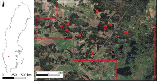
The study area is located in Remningstorp (Figure 1), Västra Götaland, Sweden (58°27′18.35″N, 13°39′8.03″E) and covers an area of 1602 ha. The forest in this area is mainly managed spruce (Pinus Sylvestris) and pine (Picea Abies) for wood production.

Figure 1. Study area and plot positions. Red polygon on the right is the laser-scanned area

2.2. Field data

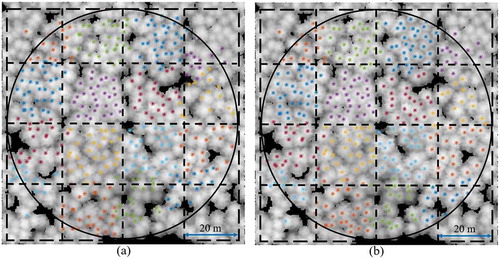
A field inventory was conducted in 2014 in 40 circular plots with diameters of 80 m. Each plot was divided into 16 subplots (20 × 20 m, Figure 3), and the positions of the subplot centres were determined with an RTK-GPS (Trimble Inc., Sunnyvale, CA, USA). The position, diameter at breast height (DBH), and species of each tree in each subplot was recorded. Individual-tree positions were determined using a Postex system (Lämås 2010) and calibrated using TLS data acquired in 2016. The height of a subsample of trees in the plots was also measured and recorded.

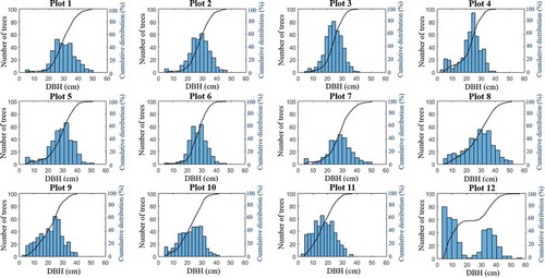
In the time between the field inventory and laser scanning, selective cutting and clear cutting were performed in 28 of the total 40 plots; only data for the 12 unchanged plots are considered here. Descriptive statistics for these plots are presented in Table 1. Because detecting understorey trees is challenging, an index was created to quantify the proportion of small trees. Here, small trees are defined as trees with DBH smaller than T, where T is the mean of the largest and smallest measured DBH for the plot. The reason for creating the index is further discussed later related to the performance of the ITD algorithm. For presentational purposes, the plot numbers were ordered according to the proportion of small trees. DBH distributions and cumulative curves are presented in Figure 2.

Table 1. Basic information about the 12 plots, including mean DBH and height, stem density, proportion of pine trees, and proportion of small trees. SD refers to standard deviation

Plot no.	Mean DBH (cm)	SD DBH/Mean DBH	Mean height (m)	SD height/Mean height	Number of stems/ha	Proportion of spruce/pine/deciduous (%)	Proportion of small trees (%)
1	30.2	0.24	21.8	0.16	615	93/1/6	24
2	28.3	0.24	21.2	0.17	704	95/0/5	27
3	24.4	0.24	19.7	0.17	921	68/3/29	28
4	22.6	0.33	18.3	0.25	905	85/0/15	29
5	28.8	0.29	21.2	0.2	740	91/0/9	31
6	27.4	0.22	19.5	0.15	635	49/49/2	32
7	28.2	0.29	20.9	0.21	543	93/0/7	35
8	28.3	0.36	20.7	0.25	820	92/0/8	38
9	21.5	0.38	17.6	0.28	899	77/1/22	44
10	22.2	0.35	17.9	0.25	808	49/0/51	46
11	17.1	0.42	14.7	0.33	1068	86/0/14	60
12	20.2	0.69	14.0	0.51	800	52/40/8	60

Figure 2. The DBH distribution of plots 1 − 12

The precision of the tree positions in each subplot relative to the subplot centres was high when using a Postex ultrasound system (Lämås 2010), but the accuracy of the subplot centres position had potentially larger errors due to the errors in the RTK-GPS measurements below the canopy (Olofsson, Lindberg, and Holmgren 2008). Consequently, all tree positions in the same subplot had an identical shift relative to the ALS data. These shifts were detected and eliminated by visual interpretation of the tree positions relative to the local maxima of the ALS data. A shift vector was added to the coordinates of all trees in each subplot, as shown in Figure 3.

Figure 3. Corrections of the single-tree positions in a representative plot. (a) Measured tree positions. (b) Corrected tree positions. The background rasters represent the output of the smoothed nDSM. The black solid lines indicate the plot’s boundary. The dotted lines show the boundaries of the 20 m × 20 m subplots

2.3. MS-ALS data

The study area was scanned on the 21 July 2016 with an Optech Titan (Teledyne Optech, Canada) commercial multispectral airborne laser scanner. This instrument scans at three laser wavelengths: 1550 nm (channel 1; short-wave infrared), 1064 nm (channel 2; near-infrared), and 532 nm (channel 3; green). To collect point cloud data with high resolution and high intensity, scanning was conducted at an altitude of around 400 m above ground level, generating 10 returns per m² in each channel, and up to four returns for each emitted pulse.

3. Methods

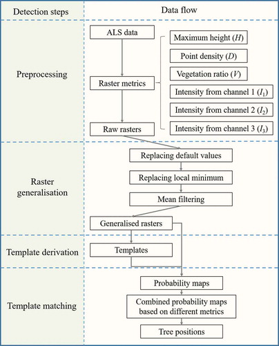
The framework of the ITD method and the study purpose are shown in Figure 4.

Figure 4. Framework of the ITD method tested here and questions considered when analysing the results

3.1. Preprocessing of laser data and raster derivation

The MS-ALS data were cut out with a 5 m buffer around the boundary of each 80 m diameter plot. The height was normalized to the ground and points lower than 2 m above the ground were removed using LAStools (2007–2020, rapidlasso GmbH, Germany) with the default settings. Range correction was done by multiplying the intensity by the squared distance to the scanner for each point.

Six raster images with 0.25 m resolution were derived from the point clouds based on the maximum height (H), point density (D), vegetation ratio (V), and average intensity from three channels (I₁, I₂, and I₃). To minimize the number of missing data cells in the raster images, the point clouds from the three channels were combined when calculating the maximum height, point density and vegetation ratio. Points less than 2 m above ground level were excluded from the point clouds when computing metrics, and the vegetation ratio was calculated as the ratio of the number of points 2 m or more above ground level to the total number of points.

3.2. Individual tree detection

3.2.1. Image generalization

Before template matching, raster cells with missing data and local minima were filled in the raster images and then smoothed to improve performance. Because of the chosen flight and scanning directions, there were missing data and minimal values between adjacent scan lines. Figure 5a depicts the scanning process and shows how the raster images are orientated with respect to the flight and scanning directions, as well as the missing data and minimal value stripes in a representative raster. To prevent the missing data and minimal values from affecting template matching, missing data cells were filled by computing the mean of all data-containing neighbouring cells in a 3 × 3 grid centred on the cell with missing data. Cells with values lower than their transverse two neighbour were replaced by the average of the two neighbours. Finally, the raster images were smoothed using a 3 × 3 mean filter.

Figure 5. The flight and scanning direction of the MS-ALS data used in this study and the generated point cloud. (a) Flight and scanning direction (i) shown on a maximum height raster (ii). (b) The corresponding point cloud seen from different directions

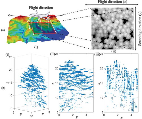
3.2.2. Template derivation

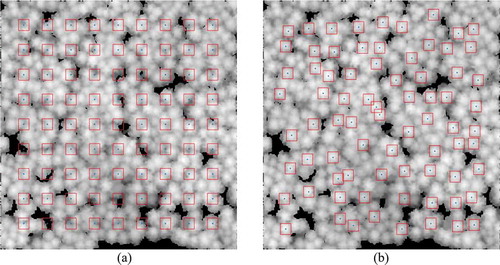
Template raster images with trees were derived directly from the rasters without using field measurements as reference data. According to the principle that a local height maximum has a high probability of being a tree top, a number of local maxima were defined as the centres of template images. For the plot size considered in this study, an n × n grid was created and the positions of the nodes were set as the initial seeds. The seeds were repeatedly moved to the adjacent raster cell with the highest value in a 2 m × 2 m neighbourhood until their positions no longer changed. Seeds whose initial placements corresponded to a gap in the canopy were excluded. Finally, 4 m × 4 m template images were defined based on the metric images of the plot, using the retained seeds as the centre (see Figure 6 for an example). During this process, it was possible for multiple initial seeds to converge onto the same local maximum, so the final number of templates could be lower than the initial one. The number of grid nodes used to create the initial seeds was varied from 1 to 15 × 15 to determine how such variation affected detection accuracy.

Figure 6. Templates (9 × 9) on a height raster image. (a) Initial positions of the nodes. (b) Final positions of the templates. Red boxes delineate the borders of the templates and blue spots indicate their centres. The background rasters are the M_DSM processed after the image generation steps proposed in.Section 3.2.1

3.2.3. Template matching

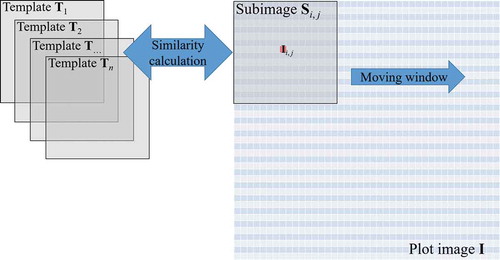
For each 90 m × 90 m plot, a similarity map with 0.25 m resolution was created using a moving window to illustrate the probability of each pixel being a tree position based on the templates (Figure 7). For a given pixel ${\mathrm{I}}_{i,j}$ in a plot image $\mathrm{I}$ a 4 m × 4 m subimage ${\mathbf{S}}_{i,j}$ centred on ${\mathrm{I}}_{i,j}$ was compared to each of the templates ${\mathbf{T}}_1$, ${\mathbf{T}}_2$ … ${\mathbf{T}}_m$ generated from a fixed number of nodes. The similarity was then calculated using Equations (1)(1) ${\mathbf{D}}_m\left(i,j\right)=\sum _{a=1}^A\sum _{b=1}^B{\left[{\mathbf{S}}_{i,j}\left(a,b\right)-{\mathbf{T}}_m\left(a,b\right)\right]}^2$(1) and (2(2) $\mathbf{P}\left(i,j\right)=1-{\left\{{\mathbf{D}}_m\left(i,j\right)\right\}}_{\mathrm{m}\mathrm{i}\mathrm{n}},m=1,2,\dots ,n$(2) )

(1) ${\mathbf{D}}_m\left(i,j\right)=\sum _{a=1}^A\sum _{b=1}^B{\left[{\mathbf{S}}_{i,j}\left(a,b\right)-{\mathbf{T}}_m\left(a,b\right)\right]}^2$(1)

(2) $\mathbf{P}\left(i,j\right)=1-{\left\{{\mathbf{D}}_m\left(i,j\right)\right\}}_{\mathrm{m}\mathrm{i}\mathrm{n}},m=1,2,\dots ,n$(2)

Figure 7. The similarity calculation process

where ${\mathbf{D}}_m\left(i,j\right)$ is the difference between subimage ${\mathbf{S}}_{i,j}$ and template ${\mathbf{T}}_m$, ${\left\{{\mathbf{D}}_m\left(i,j\right)\right\}}_{\mathrm{m}\mathrm{i}\mathrm{n}}$ is the minimum difference for all $n$ templates, and $\mathbf{P}\left(i,j\right)$ is the similarity of the pixel $\left(i,j\right)$ to a tree position. $\mathbf{S}$ and $\mathbf{T}$ were normalized against their maximum values, respectively, before calculating differences.

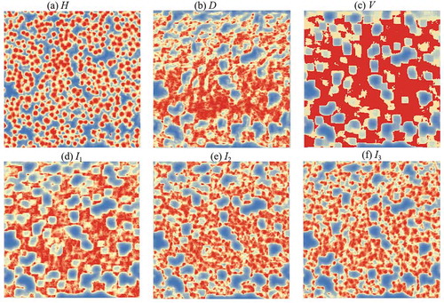
Using the same method, similarity maps (Figure 8) were derived from H, D, V, I₁, I₂, and I₃. To synthesize the similarities for different metrics, new similarity maps were created by averaging different combinations of H, D, V, I₁, I₂ and I₃. The averaged combinations are denoted P with used variables (H, D, V, I₁, I₂, and I₃) marked as subscript, e.g. P_{H, D} represents that the similarity maps from H and D are averaged for the template matching.

Figure 8. Similarly maps derived from different metrics by template matching. (a – e) H, D, V, I₁, I₂ and I_3. Red and blue indicate high and low values, respectively. Histogram equalization was performed to improve the visualization of the results

Finally, tree positions were detected from the similarity maps. The similarity maps were smoothed using a 3 × 3 Gaussian function, and a 3 × 3 moving window was used to detect the local maxima. For comparative purposes, tree positions were also detected directly from the nDSM generated using the preprocessing method described in section 3.1. The resulting tree positions are indicated by the label M_DSM in the results section.

3.3. Validation

To validate the detection accuracy, tree positions derived from ALS (ALS-trees) were matched to the field measurements (field-trees). The ALS-trees were first linked to all possible field-trees within a certain distance, then only the linked pairs with the smallest distances were retained for each tree. For trees with DBH values below 25 cm, the maximum linking distance was 3 m horizontally, while for larger trees the maximum distance was 12 × DBH (Olofsson, Lindberg, and Holmgren 2008). After matching, only trees within 35 m of the plot centres were used to assess the detection accuracy to reduce the statistical impact of trees close to the plot boundary. Precision, recall, and F-scores were calculated using Equations (3)(3) $P=\frac{\mathrm{N}\mathrm{u}\mathrm{m}\mathrm{b}\mathrm{e}\mathrm{r}\mathrm{o}\mathrm{f}\mathrm{m}\mathrm{a}\mathrm{t}\mathrm{c}\mathrm{h}\mathrm{e}\mathrm{d}\mathrm{t}\mathrm{r}\mathrm{e}\mathrm{e}\mathrm{s}}{\mathrm{N}\mathrm{u}\mathrm{m}\mathrm{b}\mathrm{e}\mathrm{r}\mathrm{o}\mathrm{f}\mathrm{t}\mathrm{r}\mathrm{e}\mathrm{e}\mathrm{s}\mathrm{d}\mathrm{e}\mathrm{t}\mathrm{e}\mathrm{c}\mathrm{t}\mathrm{e}\mathrm{d}\mathrm{b}\mathrm{y}\mathrm{A}\mathrm{L}\mathrm{S}}$(3) – (5(5) $F=\frac{2\times P\times R}{P+R}$(5) ):

(3) $P=\frac{\mathrm{N}\mathrm{u}\mathrm{m}\mathrm{b}\mathrm{e}\mathrm{r}\mathrm{o}\mathrm{f}\mathrm{m}\mathrm{a}\mathrm{t}\mathrm{c}\mathrm{h}\mathrm{e}\mathrm{d}\mathrm{t}\mathrm{r}\mathrm{e}\mathrm{e}\mathrm{s}}{\mathrm{N}\mathrm{u}\mathrm{m}\mathrm{b}\mathrm{e}\mathrm{r}\mathrm{o}\mathrm{f}\mathrm{t}\mathrm{r}\mathrm{e}\mathrm{e}\mathrm{s}\mathrm{d}\mathrm{e}\mathrm{t}\mathrm{e}\mathrm{c}\mathrm{t}\mathrm{e}\mathrm{d}\mathrm{b}\mathrm{y}\mathrm{A}\mathrm{L}\mathrm{S}}$(3)

(4) $R=\frac{\mathrm{N}\mathrm{u}\mathrm{m}\mathrm{b}\mathrm{e}\mathrm{r}\mathrm{o}\mathrm{f}\mathrm{m}\mathrm{a}\mathrm{t}\mathrm{c}\mathrm{h}\mathrm{e}\mathrm{d}\mathrm{t}\mathrm{r}\mathrm{e}\mathrm{e}\mathrm{s}}{\mathrm{N}\mathrm{u}\mathrm{m}\mathrm{b}\mathrm{e}\mathrm{r}\mathrm{o}\mathrm{f}\mathrm{t}\mathrm{r}\mathrm{e}\mathrm{e}\mathrm{s}\mathrm{r}\mathrm{e}\mathrm{c}\mathrm{o}\mathrm{r}\mathrm{d}\mathrm{e}\mathrm{d}\mathrm{i}\mathrm{n}\mathrm{t}\mathrm{h}\mathrm{e}\mathrm{f}\mathrm{i}\mathrm{e}\mathrm{l}\mathrm{d}\mathrm{i}\mathrm{n}\mathrm{v}\mathrm{e}\mathrm{n}\mathrm{t}\mathrm{o}\mathrm{r}\mathrm{y}}$(4)

(5) $F=\frac{2\times P\times R}{P+R}$(5)

In this study, F-scores were used for parameter comparison and selection in Section 4.1 and 4.2 because it is a comprehensive evaluation of the commission and omission effects. In Section 4.3 where presenting the detection accuracy, detection rate (R_D, same value as R in Eq. 4)(4) $R=\frac{\mathrm{N}\mathrm{u}\mathrm{m}\mathrm{b}\mathrm{e}\mathrm{r}\mathrm{o}\mathrm{f}\mathrm{m}\mathrm{a}\mathrm{t}\mathrm{c}\mathrm{h}\mathrm{e}\mathrm{d}\mathrm{t}\mathrm{r}\mathrm{e}\mathrm{e}\mathrm{s}}{\mathrm{N}\mathrm{u}\mathrm{m}\mathrm{b}\mathrm{e}\mathrm{r}\mathrm{o}\mathrm{f}\mathrm{t}\mathrm{r}\mathrm{e}\mathrm{e}\mathrm{s}\mathrm{r}\mathrm{e}\mathrm{c}\mathrm{o}\mathrm{r}\mathrm{d}\mathrm{e}\mathrm{d}\mathrm{i}\mathrm{n}\mathrm{t}\mathrm{h}\mathrm{e}\mathrm{f}\mathrm{i}\mathrm{e}\mathrm{l}\mathrm{d}\mathrm{i}\mathrm{n}\mathrm{v}\mathrm{e}\mathrm{n}\mathrm{t}\mathrm{o}\mathrm{r}\mathrm{y}}$(4) was used for better cross-interpretation of results from different studies. Specially, the detection rate of the small trees (R_D,s) was also presented to show the performance of understorey detection.

4. Results

4.1. Generalization of raster images

Figure 9 shows representative rasters generated during each of the generalization steps based on data for Plot 1. For height rasters, replacing missing data values had a clear effect in that it eliminated striped texture from the images. However, the striped texture in the density and vegetation ratio rasters only disappeared after replacing low values. In the case of the intensity rasters (particularly those for channels 1 and 2), it was difficult to distinguish tree crowns in the original images, and all generalization steps improved the detection of treetops and crown boundaries.

Figure 9. The effects of the processing steps on rasters based on different metrics within a 25 × 25 m area

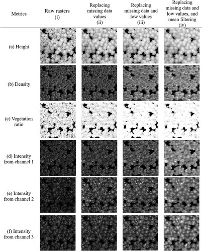
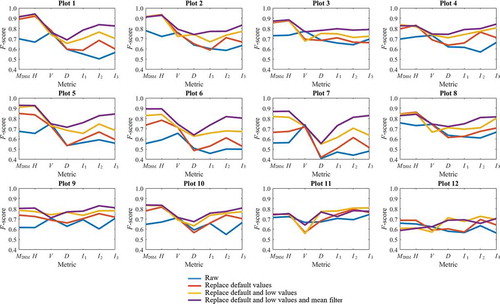
The quantitative description of how each generalization step improved the detection performance was conducted using F-scores (Figure 10). Consistent with Figure 9, different metrics showed significant different improvements within each step. For M_DSM and H, F-scores increased most obviously when only replacing default values, while replacing the low values and mean filter did not contribute much. However, for density, only replacing default values showed little improvements compared to the raw data, while replacing low values was the most crucial step for all plots. For intensity, especially I₂ and I₃, F-scores improved significantly after every step, illustrating the necessity of conducting every step in the generalization.

Figure 10. F-scores for all plots based on individual metrics: M_DSM, H, V, D, I₁, I₂ and I_3.

4.2. Template derivation

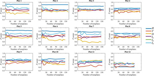
The numbers of templates generated using different numbers of nodes, and the corresponding precision values, are given in Table A1 and Table A2 in Appendix. Higher numbers of nodes resulted in the generation of more templates and increased the probability of fake templates emerging (i.e. templates that could not be matched to field-measured trees). However, such fake templates did not reduce the detection accuracy, as shown in Figure 11. For example, even when one in three templates was fake for Plot 10, the F-scores were not appreciably lower than in cases without fake templates. However, additional templates did not improve the detection accuracy; broadly speaking, the detection was insensitive to the number of templates.

Figure 11. F-scores for detection using different numbers of templates

4.3. Detection accuracy

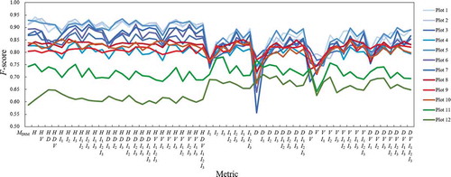
The detection accuracy values presented in this section are based on rasters obtained after applying all generalization steps and a 9 × 9 grid for template derivation. All results for individual and combined metrics for the 12 plots are presented in Figure 12. For all plots, template matching from H improved accuracy relative to detecting local maxima directly from the generalized nDSM. The effects of combining metrics on accuracy differed between plots. For plots 1–7 (see blue lines in Figure 12), the F-scores were highest using combinations containing H and particularly low for combinations including D. For plots 11–12 (green lines), performance was best for combinations including D but not H. Plots 8–10 (red lines) behaved similarly to plots 1–7 but yielded better performance when template matching was done using I instead of H or D.

Figure 12. F-scores using different metrics/combined metrics for 12 plots

The different performances of H, D and I for plots with different structures could be explained by the raster textures (Figures 13 and 14). Figure 13 presents an example of a small tree standing beside a dominant tree in Plot 12, which had 60% small trees. The H raster (Figure 13b) shows significantly lower values for the small tree compared to the surroundings, leading to difficulty of detection. However, in the rasters of density and intensity, the pixel values of small trees were influenced only slightly by the dominant tree. This example illustrates that the rasters of density and intensity provided more possibilities for detecting small trees beside dominant trees.

Figure 13. An example for a small tree standing beside a dominant tree in Plot 12. (a) 3D point cloud from laser data. (b) rasters of (i) H, (ii) D, (iii) I₂ and (iv) I₃. Red asterisks and blue circles indicate field-measured trees and detected trees, respectively; blue lines represent the links between them. Yellow cycle makes out the small tree in different rasters

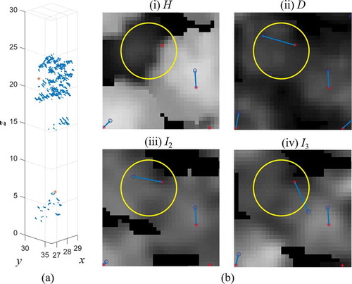
Figure 14. An example for several understorey trees standing under a dominant tree in Plot 12. (a) 3D point cloud from laser data. (b) rasters of (i) H, (ii) D, (iii) I₂ and (iv) I₃. Red asterisks and blue circles indicate field-measured trees and detected trees, respectively; blue lines represent the links between them

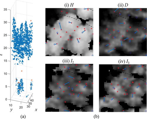
For the cases of understorey trees, Figure 14 shows an example of how D and I improved the detection rate. The returns from the understorey trees changed D and I, causing more fragmentized texture compared to H, improving the probability of detecting understorey trees. Instead of only focusing on the top layer as H, D and I were more sensitive to the point cloud from different vertical layers.

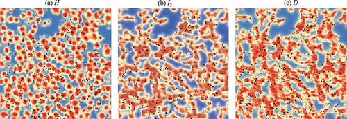
Figure 15 shows the similarity maps for the height (H), intensity of the 1064 nm channel (I₂), and point density (D) for Plot 12. The similarity map for H looks similar to the nDSM, only showing the tallest layer of the canopy. The similarity map for I₂ exhibits higher values connecting the tree crowns around small trees, and the similarity map for D exhibits greater variation in the regions containing small trees, resulting in more local maxima. Although D provided more information that could be used to detect understorey trees, it was less easy to generalize than H, as shown in Figure 11; the D rasters had too much texture inside the tree crowns (Figure 9), which also might lead to over-segmentation.

Figure 15. Similarity maps for (a) H, (b) I₂ and (c) D in Plot 12. Red and blue indicate high and low values, respectively; black points indicate the positions of trees according to field measurements

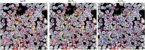
When combining the similarity maps from different metrics, the performance of detection improved with the average effects among different metrics. Figure 16 depicts the linkage of ALS-trees and field-trees for Plot 12; the yellow boxes highlight regions with notable differences. It is clear that P_{I2, I3} was better at detecting small trees standing at the edges of big tree crowns. However, for clusters of small trees under big tree crowns (highlighted using green boxes), intensity was insufficient for detection. In such cases, the density and vegetation ratio were excellent for detecting clusters of small trees.

Figure 16. Linkage between trees detected by template matching and field-measured trees using the (a) H, (b) P_{I2, I3} and (c) P_{D, V} metrics for Plot 12. Red asterisks and blue circles indicate field-measured trees and detected trees, respectively; blue lines represent the links between them. The background rasters are the nDSM processed after the image generation steps proposed in.Section 3.2.1

To identify metric combinations suitable for use in plots with different forest structures, we considered the combinations with the highest and second highest accuracy for each plot (collectively referred to as top accuracies). We then selected the metric combinations with the most top accuracy results for plots with similar proportions of small trees. Table 2 summarizes the accuracies achieved with different combinations and the optimal combinations selected for different plot types. When detailed information on the plot conditions is available, the metric combinations listed under Option 1 in Table 2 are recommended; this option provides five different metric selections for five kinds of plot conditions. Option two represents a simplified solution for three levels of canopy complexity. For comparative purposes, Table 2 also shows the accuracy achieved using local maxima detection, which is a commonly used ITD method.

Table 2. Summary of the plot attributes, optimal metric combinations for single tree detection in each plot, the accuracy achieved using these combinations, and the accuracy achieved by direct detection based on local maxima for each plot

Plot no.	Proportion of small trees (%)	Template matching								Local maxima detection
		Option 1				Option 2
		Metrics	F-scores	RD	RD,s	Metrics	F-scores	RD	RD,s	F-scores	RD	RD,s
1	24	H	0.94	0.90	0.82	PH, I2, I3	0.93	0.90	0.82	0.91	0.87	0.72
2	27	H	0.93	0.89	0.68	PH, I2, I3	0.92	0.89	0.72	0.91	0.86	0.61
3	28	H	0.88	0.83	0.67	PH, I2, I3	0.88	0.86	0.73	0.87	0.81	0.64
4	29	H	0.83	0.73	0.42	PH, I2, I3	0.83	0.72	0.42	0.83	0.73	0.39
5	31	H	0.93	0.89	0.69	PH, I2, I3	0.93	0.89	0.75	0.93	0.89	0.72
6	32	PH, I2, I3	0.90	0.88	0.83	PH, I2, I3	0.90	0.88	0.83	0.89	0.87	0.84
7	35	PH, I2, I3	0.91	0.89	0.77	PH, I2, I3	0.91	0.89	0.77	0.87	0.90	0.75
8	38	PV, I2, I3	0.85	0.79	0.60	PH, I2, I3	0.84	0.75	0.52	0.83	0.72	0.47
9	44	PV, I2, I3	0.85	0.77	0.65	PI2, I3	0.85	0.81	0.72	0.80	0.73	0.52
10	46	PV, I2, I3	0.85	0.84	0.74	PI2, I3	0.84	0.87	0.81	0.84	0.73	0.56
11	60	I3	0.78	0.69	0.59	I2	0.77	0.70	0.61	0.74	0.61	0.46
12	60	PD, V	0.73	0.68	0.56	I2	0.69	0.59	0.46	0.59	0.44	0.24

5. Discussion

In this study, the individual tree detection (ITD) performance of MS-ALS was tested in plots with varying forest structures. ITD performance was evaluated on the basis of six metrics (height, point density, vegetation ratio, and intensity from three channels) and various combinations of these metrics. Height is the metric most commonly used for ITD based on ALS data (Eysn et al. 2015; Sačkov, Kulla, and Bucha 2019; Aubry-Kientz et al. 2019) even though its limitations with respect to detecting understorey trees have been widely noted. The results presented here show that this deficiency can be overcome by using additional metrics. The inclusion of intensity substantially improved ITD performance for some plots, demonstrating the advantages of MS-ALS over single-wavelength ALS.

In this study, the best metric differed between the plots. Therefore, rules for metric selection were proposed based on an analysis of the plots’ forest structure. Two main groups of plots were identified: ITD based on H yielded the best performance for plots 1–7, which had a typical sigmoidal cumulative DBH distribution curve (shown in Figure 2), whereas for plots with more small trees, ITD based on intensity or density yielded better results. To provide quantitative guidance when selecting metrics for ITD, an index was defined based on the proportion of small trees in a plot. When this index was low, height was sufficient to identify most trees. Conversely, in plots with high values of this index, intensity should be included to improve the detection of small trees beside or beneath the crowns of large trees, and height should have less weight. When this index reached 60%, performance was improved by including the point density metric because of the high point density associated with small tree groups. The index used in this study was derived from the DBH, but indicators reflecting the vertical complexity of the canopy structure could also be derived from the ALS point cloud (Coops et al. 2016; Wilkes et al. 2016). Future studies could use such indices as criteria for selecting raster metrics for ITD.

The template matching method developed in this study involves generating templates from the target data. In other studies on ITD using template matching, templates were created using simulation models (Gulbe and Mednieks 2013; Holmgren and Lindberg 2013; Nyström et al. 2014; Pirotti 2010) or by selecting sample trees manually in the image (Gulbe and Mednieks 2013). Gulbe and Mednieks reported detection rates of 56% and 71%, respectively, using these two types of templates. In this study, the templates were automatically derived from the height rasters. Local height maxima have a rather high probability of corresponding to tree positions, as shown in Table A2. This approach enabled fully automated detection without requiring manual interaction. Another benefit of the consistent generalization strategy was that crown shape deviations in both templates and the target plot data were eliminated to the same degree, reducing sensitivity to template shapes and textures. Figure 11 shows that using generalized rasters made the detection accuracy sufficiently stable with respect to variation in the number of templates, eliminating the need to determine the optimal number of templates.

Generalization of rasters has been a common preprocessing step in ITD, while the step of compensation of local low values used in this study was newly proposed for template matching for ITD. Although the local low values contained certain texture information of individual crowns, the additional texture within crowns might disturb the detection of the crown edges, which were more crucial for ITD. In addition, the random local low values also decreased the generalized level of templates. In this study, similarity maps based on different metrics were averaged by applying the same weighting to all the included metrics. In the future, it may be desirable to optimize the weightings of the metrics based on the forest structure and to thoroughly assess the similarity between target and template rasters for height, point density, and intensity distribution.

6. Conclusion

In this study, ITD from MS-ALS data was conducted, resulting in a detection rate of 0.90 to 0.68 for different forest structures. The performance of ITD was compared for different metrics, including height, point density, vegetation ratio, and intensity from three channels. For homogeneous forest stands, height remained the best and most easily used metric for ITD, but metrics such as intensity and density yielded better performance than height for forests with complex structures. For the plot with the most understorey trees in this study, ITD based on point density and vegetation ratio yielded 0.32 higher detection rate of small trees than local maxima detection based on height.

In addition, a framework for ITD based on a template matching algorithm was developed. Deriving templates from the target plot instead of field data or manual selection was shown to be feasible. The image generalization flow presented here increased the robustness among different metrics. The compensation for the local low values was shown to be crucial for generalizing density and intensity metrics.

This study has confirmed that the additional spectral information provided by MS-ALS compared to single-wavelength ALS can significantly improve the detection of understorey trees. Using intensity metrics from laser data can be a basis for other ITD algorithms. Future studies can be conducted on forests with even more layers to explore how the intensity metrics respond to the canopy layers. Additionally, more ITD methods can be developed using the point density distribution, which showed annular textures for individual trees in this study. The pixels with abnormal increasing density in the annular textures have high potential to be used for detecting understorey trees.

Contributions

All authors conceived and designed the study, analyzed the results and wrote the manuscript; Langning Huo improved and implemented the algorithm.

Acknowledgements

The data from field inventory and the laser scanning were supported by the Hildur and Sven Wingquist Foundation for Forest Science Research. We would like to thank Dr Johan Holmgren, who contributed to the study’s design.

Disclosure statement

The authors declare no conflict of interest.

Additional information

Funding

This work was supported by the Hildur and Sven Wingquist Foundation.

References

- Ahokas, E., J. Hyyppä, X. Yu, X. Liang, L. Matikainen, K. Karila, P. Litkey, et al. 2016. “Towards Automatic Single-sensor Mapping by Multispectral Airborne Laser Scanning.” International Archives of the Photogrammetry, Remote Sensing and Spatial Information Sciences XLI-B3:155–162.
- Aubry-Kientz, M., R. Dutrieux, A. Ferraz, S. Saatchi, H. Hamraz, J. Williams, D. Coomes, A. Piboule, and G. Vincent. 2019. “A Comparative Assessment of the Performance of Individual Tree Crowns Delineation Algorithms from ALS Data in Tropical Forests.” Remote Sensing 11 (9): 1086. doi:10.3390/rs11091086.
- Axelsson, A., E. Lindberg, and H. Olsson. 2018. “Exploring Multispectral ALS Data for Tree Species Classification.” Remote Sensing 10 (3): 183. doi:10.3390/rs10020183.
- Breidenbach, J., E. Næsset, V. Lien, T. Gobakken, and S. Solberg. 2010. “Prediction of species specific forest inventory attributes using a nonparametric semi-individual tree crown approach based on fused airborne laser scanning and multispectral data.” Remote Sensing of Environment 114 (4): 911–924. doi:10.1016/j.rse.2009.12.004.
- Budei, B. C., B. St-Onge, C. Hopkinson, and F.-A. Audet. 2018. “Identifying the Genus or Species of Individual Trees Using a Three-wavelength Airborne Lidar System.” Remote Sensing of Environment 204: 632–647.
- Coops, N. C., P. Tompaski, W. Nijland, G. J. M. Rickbeil, S. E. Nielsen, C. W. Bater, and J. J. Stadt. 2016. “A Forest Structure Habitat Index Based on Airborne Laser Scanning Data.” Ecological Indicators 67: 346–357.
- Ene, L., E. Næsset, and T. Gobakken. 2012. “Single tree detection in heterogeneous boreal forests using airborne laser scanning and area-based stem number estimates.” International Journal of Remote Sensing 33 (16): 5171–93. doi: 10.1080/01431161.2012.657363.
- Eysn, L., M. Hollaus, E. Lindberg, F. Berger, J.-M. Monnet, M. Dalponte, M. Kobal, et al. 2015. “A Benchmark of Lidar-Based Single Tree Detection Methods Using Heterogeneous Forest Data from the Alpine Space.” Forests 6 (12): 1721–1747. doi:10.3390/f6051721.
- Gong, W., J. Sun, S. Shi, J. Yang, D. Lin, B. Zhu, and S. Song. 2015. “Investigating the Potential of Using the Spatial and Spectral Information of Multispectral LiDAR for Object Classification.” Sensors (Basel, Switzerland) 15 (9): 21989–22002. doi:10.3390/s150921989.
- Gulbe, L., and I. Mednieks. 2013. “Automatic Identification of Individual Tree Crowns in Mixed Forests Using Fusion of LIDAR and Multispectral Data.” Technologies of Computer Control Vol.14: 93–99.
- Gupta, S., H. Weinacker, and B. Koch. 2010. “Comparative Analysis of Clustering-Based Approaches for 3-D Single Tree Detection Using Airborne Fullwave Lidar Data.” Remote Sensing 2 (4): 968–989. doi:10.3390/rs2040968.
- Heinzel, J., and B. Koch. 2012. “Investigating Multiple Data Sources for Tree Species Classification in Temperate Forest and Use for Single Tree Delineation.” International Journal of Applied Earth Observation and Geoinformation 18: 101–110.
- Holmgren, J., and E. Lindberg. 2013. “Tree Crown Segmentation Based on a Geometric Tree Crown Model for Prediction of Forest Variables.” Canadian Journal of Remote Sensing 39 (sup1): S86–S98. doi:10.5589/m13-025.
- Hyyppa, J., O. Kelle, M. Lehikoinen, and M. Inkinen. 2001. “A segmentation-based method to retrieve stem volume estimates from 3-D tree height models produced by laser scanners.” IEEE Trans. Geosci. Remote Sensing 39 (5): 969–975. doi:10.1109/36.921414.
- Junttila, S., J. Sugano, M. Vastaranta, R. Linnakoski, H. Kaartinen, A. Kukko, M. Holopainen, H. Hyyppä, and H. Juha. 2018. “Can Leaf Water Content Be Estimated Using Multispectral Terrestrial Laser Scanning? A Case Study with Norway Spruce Seedlings.” Frontiers in Plant Science 9: 299.
- Junttila, S., M. Vastaranta, X. Liang, H. Kaartinen, A. Kukko, S. Kaasalainen, M. Holopainen, H. Hyyppä, and H. Juha. 2017. “Measuring Leaf Water Content with Dual-Wavelength Intensity Data from Terrestrial Laser Scanners.” Remote Sensing 9 (1): 8. doi:10.3390/rs9010008.
- Ke, Y., L. J. Quackenbush, and J. Im.2010. “Synergistic use of QuickBird multispectral imagery and LIDAR data for object-based forest species classification.” Remote Sensing of Environment 114 (6): 1141–1154. doi: 10.1016/j.rse.2010.01.002.
- Kestur, R., A. Angural, B. Bashir, S. N. Omkar, G. Anand, and M. B. Meenavathi. 2018. “Tree Crown Detection, Delineation and Counting in UAV Remote Sensed Images: A Neural Network Based Spectral–Spatial Method.” Journal of the Indian Society of Remote Sensing 46 (6): 991–1004. doi:10.1007/s12524-018-0756-4.
- Lämås, T. 2010. “The Haglöf PosTex Ultrasound Instrument for the Positioning of Objects on Forest Sample Plots.” 296.
- Larsen, M., M. Eriksson, X. Descombes, G. Perrin, T. Brandtberg, and F. A. Gougeon. 2011. “Comparison of Six Individual Tree Crown Detection Algorithms Evaluated under Varying Forest Conditions.” International Journal of Remote Sensing 32 (20): 5827–5852. doi:10.1080/01431161.2010.507790.
- Larsen, M., and M. Rudemo. 1998. “Optimizing Templates for Finding Trees in Aerial Photographs.” Pattern Recognition Letters 19 (12): 1153–1162. doi:10.1016/S0167-8655(98)00092-0.
- Leckie, D. G., F. A. Nicholas Walsworth, S. G. Gougeon, D. Johnson, L. Johnson, K. Oddleifson, D. Plotsky, and V. Rogers. 2016. “Automated Individual Tree Isolation on High-Resolution Imagery: Possible Methods for Breaking Isolations Involving Multiple Trees.” IEEE Journal of Selected Topics in Applied Earth Observations and Remote Sensing 9 (7): 3229–3248. doi:10.1109/JSTARS.2016.2544109.
- Leckie, D., F. Gougeon, D. Hill, R. Quinn, L. Armstrong, and R. Shreenan. 2003. “Combined high-density lidar and multispectral imagery for individual tree crown analysis.” Canadian Journal of Remote Sensing 29 (5): 633–649. doi:10.5589/m03-024.
- Lee, H., K. C. Slatton, B. E. Roth, and W. P. Cropper. 2010. “Adaptive clustering of airborne LiDAR data to segment individual tree crowns in managed pine forests.” International Journal of Remote Sensing 31 (1): 117–139. doi:10.1080/01431160902882561.
- Lindberg, E., J. Holmgren, K. Olofsson, J. Wallerman, and H. Olsson. 2013. “Estimation of Tree Lists from Airborne Laser Scanning Using Tree Model Clustering and k-MSN Imputation.” Remote Sensing 5 (4): 1932–1955. doi:10.3390/rs5041932.
- Matikainen, L., K. Karila, J. Hyyppä, E. Puttonen, P. Litkey, and E. Ahokas. 2017. “Feasibility of Multispectral Airborne Laser Scanning for Land Cover Classification, Road Mapping and Map Updating.” International Archives of the Photogrammetry, Remote Sensing and Spatial Information Sciences XLII-3/W3: 119–122.
- Morsy, S., A. Shaker, A. El-Rabbany, and P. E. LaRocque. 2016. “Airborne Multispectral Lidar Data for Land-cover Classification and Land/water Mapping Using Different Spectral Indexes.” ISPRS Annals of the Photogrammetry, Remote Sensing and Spatial Information Sciences III-3: 217–224.
- Nyström, M., J. Holmgren, J. E. S. Fransson, and H. Olsson. 2014. “Detection of Windthrown Trees Using Airborne Laser Scanning.” International Journal of Applied Earth Observation and Geoinformation 30: 21–29.
- Olofsson, K., E. Lindberg, and J. Holmgren, eds. 2008. A Method for Linking Field-surveyed and Aerial-detected Single Trees Using Cross Correlation of Position Images and the Optimization of Weighted Tree List Graphs. Edinburgh, UK: Heriot-Watt University, SilviLaser 2008.
- Panagiotidis, D., A. Abdollahnejad, P. Surový, and K. Karel. 2019. “Detection of Fallen Logs from High-resolution UAV Images.” NZJFS 49 (3): 423.
- Pirotti, F. 2010. “Assessing a Template Matching Approach for Tree Height and Position Extraction from Lidar-Derived Canopy Height Models of Pinus Pinaster Stands.” Forests 1 (4): 194–208. doi:10.3390/f1040194.
- Pollock, R. 1996. The Automatic Recognition of Individual Trees in Aerial Images of Forests Based on a Synthetic Tree Crown Image Model. University of British Columbia. Canada, BC: Vancouver.
- Sačkov, I., L. Kulla, and T. Bucha. 2019. “A Comparison of Two Tree Detection Methods for Estimation of Forest Stand and Ecological Variables from Airborne LiDAR Data in Central European Forests.” Remote Sensing 11 (12): 1431. doi:10.3390/rs11121431.
- Solberg, S., E. Naesset, and O. M. Bollandsas. 2006. “Single Tree Segmentation Using Airborne Laser Scanner Data in a Structurally Heterogeneous Spruce Forest.” Photogramm eng remote sensing 72 (12): 1369–1378. doi:10.14358/PERS.72.12.1369.
- Tang, F., X. Zhang, and J. Liu. 2007. “Segmentation of tree crown model with complex structure from airborne LIDAR data.” In Geoinformatics 2007: Remotely Sensed Data and Information, edited by Weimin Ju and Shuhe Zhao, 67520A. SPIE Proceedings: SPIE.
- Wallace, A. M., A. McCarthy, C. J. Nichol, X. Ren, S. Morak, D. Martinez-Ramirez, I. H. Woodhouse, and G. S. Buller. 2014. “Design and Evaluation of Multispectral LiDAR for the Recovery of Arboreal Parameters.” IEEE Transactions on Geoscience and Remote Sensing 52 (8): 4942–4954. doi:10.1109/TGRS.2013.2285942.
- Wichmann, V., M. Bremer, J. Lindenberger, M. Rutzinger, C. Georges, and F. Petrini-Monteferri. 2015. “Evaluating the Potential of Multispectral Airborne Lidar for Topographic Mapping and Land Cover Classification.” ISPRS Annals of the Photogrammetry, Remote Sensing and Spatial Information Sciences II-3/W5: 113–119.
- Wilkes, P., S. D. Jones, L. Suarez, A. Haywood, A. Mellor, W. Woodgate, M. Soto-Berelov, and A. K. Skidmore. 2016. “Using Discrete-return Airborne Laser Scanning to Quantify Number of Canopy Strata across Diverse Forest Types.” Methods In Ecology And Evolution / British Ecological Society 7 (6): 700–712. doi:10.1111/2041-210X.12510.
- Xiao, W., A. Zaforemska, M. Smigaj, Y. Wang, and R. Gaulton. 2019. “Mean Shift Segmentation Assessment for Individual Forest Tree Delineation from Airborne Lidar Data.” Remote Sensing 11 (11): 1263. doi:10.3390/rs11111263.
- Yu, X., J. Hyyppä, P. Litkey, H. Kaartinen, M. Vastaranta, and M. Holopainen. 2017. “Single-Sensor Solution to Tree Species Classification Using Multispectral Airborne Laser Scanning.” Remote Sensing 9 (2): 108. doi:10.3390/rs9020108.