Detecting phenological changes in plant functional types over West African savannah dominated landscape

ABSTRACT

Phenology is an important component in the climate system, and play a key role in controlling many feedbacks of vegetation to the climate systems. Differences in phenology of plant functional types (PFTs) due to the variation in seasonal cycles (e.g. changes in weather variability), the impact from land-use activities (e.g. fire) and their mechanisms for adaptation (e.g. climate change, regrowth/post-fire regeneration) have major implications in conservation planning and monitoring actions. Detecting phenological variations in PFTs is therefore of great importance to quantitative remote sensing applications, especially in a biome as diverse and complex as savannah. In this study, we implement Savitzky–Golay filtering and the Breaks For Additive Seasonal and Trend (BFAST) algorithms to detect changes in PFTs based on their phenological events using Moderate Resolution Imaging Spectroradiometer (MODIS), normalized difference vegetation index (NDVI) data from 2001 to 2018. In this region, PFTs present distinct seasonal, annual and interannual variability. Woody phenology presents early green-up dates with a prolonged senescence period and invariably observed the longest growing season length (GSL). The relationship between the start of season (SOS) or end of season (EOS) was assessed for each PFT to find out the extent to which they determine GSL for different PFTs. GSL is mostly determined by the SOS in woody savannah (coefficient of determination (R²) =0.41, p <0.01), open shrubs and (R² =0.79, p <0.001), grassland (R² =0.35, p <0.01) while EOS determined the GSL for both dryland crops (R² =0.75, p <0.001) and paddy rice (R² =0.69, p <0.001). We compared the interannual variability of woody savannah and other PFTs by measuring the differences of their phenological indicators using Welch’s t-test. All PFTs show statistically significant difference with the GSL of woody savannah except open shrubs (p = 0.23). The abrupt vegetation changes estimated with BFAST varied by PFT. Some PFTs are more resilient to harsh environmental conditions than others. While woody species present a few abrupt changes, grass phenology is more vulnerable to disturbance, seasonally as well as in the trend components (large number of abrupt changes) with browning trend following an abrupt negative change. In all PFTs, breakpoint (disturbance) assessed using BFAST negatively correlate with precipitation data which means the magnitude of disturbance decreases with increasing precipitation. Woody species had an r (correlation coefficient) value of -0.5 while grassland had r = -0.7 which is a further indication that grass phenology responds more strongly to annual precipitation than the woody species. These results show that MODIS NDVI time-series data can be used to distinguish the phenological events of different PFTs in West African savannah dominated landscape.

KEYWORDS:

• MODIS;
• NDVI;
• phenology;
• interannual variability;
• savannah;
• vulnerability disturbance;
• plant functional types;
• BFAST;
• West Africa

1. Introduction

Phenology is the study of the timing of recurring biological events, their responses to biotic and abiotic forces, and the interactions among phases of the same or different species (Helmut 1975). Conceptionally, plant functional types (PFTs) are groups of species that show similar structural, physiological and/or phenological features, responses to environmental conditions or have similar impacts on ecosystems (Gitay and Nobel 1997; Ustin and Gamon 2010). Recently, there has been increased interest in monitoring land surface phenological changes of PFTs over various spatial and temporal scales (de Bie et al. 1998; Zhang et al. 2003; Whitecross, Witkowski, and Archibald 2016; Julius et al. 2019). In savannah dominated landscape, phenological changes are highly sensitive to climatic fluctuations due to ecosystem diversity and high interannual climate variability (e.g. the mean annual rainfall) across the landscape (Martínez and Gilabert 2009; Fensham, Fairfax, and Archer 2005). Furthermore, the savannah biome includes spatially and temporally highly complex ecosystems, where trees, shrubs, and grasses contribute to system-level functions such as primary production, carbon, water, and nutrient cycling (Hill and Hanan 2010). Variation in the phenology of PFTs (and their year to year variation) due to the variation in seasonal cycles (e.g. changes in weather variability), the impact from land cover change (e.g. fire) and their mechanisms for adaptation (e.g. climate change, regrowth/post-fire regeneration) have major implications for conservation planning and monitoring actions (Scholes and Archer 1997; Sankaran et al. 2005; Geng et al. 2019; Rapinel 2019). This is because savannah ecosystem supports unique communities of pastoral and agricultural communities alongside wild and domestic herbivores.

Even though climate, soil, species diversity, and habitat type are some of the important driving factors influencing the savannah vegetation changes (Hill et al. 2011; Cho et al. 2012; Higgins et al. 2011), human management and land use have been identified as a major contributing factor in West Africa (Ibrahim, Balzter, and Kaduk 2018; Leßmeister et al. 2019). Generally, anthropogenic factors were found to have serious negative consequences for vegetation productivity and overall climate (Valentini et al. 2014). For instance, increased deforestation, anthropogenic land fragmentation and biomass burning are causing massive land degradation (Valentini et al. 2014; Tansey et al. 2008, 2004) in many parts of Africa. In West African savannahs, population increases are exerting further pressures on the available resources particularly on land due to poverty, demand for food, shelter, and development of agro-industries. While there is a strong need for global carbon monitoring systems to understand the biophysical and socioeconomic components to determine meaningful ways of stabilizing climate through climate mitigation options and specifically the conservation of carbon pools in Africa land-use emissions are even higher than the fossil fuel emissions. Of this total, African savannah is believed to be responsible for a significant proportion of emissions due to fires (Valentini et al. 2014; Williams et al. 2007; Tansey et al. 2004)

A huge area of land in the savannah biome is dominated by grasses and dryland crops. All PFTs contribute to system-level functions such as primary production. Scholes (Scholes 2003) discussed that the managers of mixed tree-grass systems have tended to focus solely on only one of the components. If they were animal herders, their objective was to maximize grass production, and if they were foresters, it was to maximize tree production. A recent study held the view that human impacts in African savannahs are mediated by plant functional traits (Osborne et al. 2018). Therefore, quantifying the differences in PFTs in terms of seasonal, annual and interannual variability and their response to disturbance is therefore very important for conservation planning and monitoring actions but also very challenging in an ecosystem due to mixtures of trees, grasses, dryland crops, and also paddy rice.

Timely and accurate detection of land surface phenology and its variability among PFTs is also important for understanding environmental change. The detection of phenological variability is useful for understanding the interactions between human and natural systems such that better environmental policies can be designed. Time series analyses of remote sensing data (Moreno-de Las Heras et al. 2015; Vladimir et al. 2016; Rapinel 2019; Zhang et al. 2003) allow for phenological studies of vegetation to be carried out in a landscape (e.g. peak of the greening period, senescence, length of growing season, etc.), continental and global scales (Huete et al. 2002; Zhang et al. 2003; Edward et al. 2008; Ma et al. 2013). Space borne optical sensors such as the Moderate Resolution Imaging Spectroradiometer (MODIS) provide regular (daily to biweekly) measurements of a variety of biophysical and biochemical parameters of the land surface (Tucker, Townshend, and Goff 1985; Huete et al. 2002; Ma et al. 2013). The use of remote sensing data (e.g. normalized difference vegetation index (NDVI)) to monitor disturbance or retrospectively identify the effects of environmental variables on phenological variability of PFTs is receiving significant attention (Jacques et al. 2014; Andrew and Warrener 2017; Ilangakoon et al. 2018; Cao et al. 2018; Yang et al. 2018; Nguyen et al. 2018; Woodcock et al. 2019).

Despite the role of phenology in controlling many feedbacks of vegetation to the climate systems by influencing the seasonality of albedo (e.g. lower albedo in woodlands compared to grassland ecosystem), CO₂ (net carbon uptake is greater in PFTs with longer, rather than shorter growing season length (GSL)), surface roughness (varies with PFT, for example, agricultural crop experienced a substantial increase in surface roughness length over the growing season) and canopy conductance (increases with increasing leaf area index), so far, there has been little discussion about the frequency of occurrence of the early/late greening phenomenon on PFTs in African savannahs (Whitecross, Witkowski, and Archibald 2016). In this study, we focus on differentiating PFTs based on, for example, SOS, EOS, and GSL, using the NDVI as several authors have previously paid more attention to identifying plant traits based on, for example, pigments, dry matter, nitrogen, or phosphorus content which are useful to optically differentiate plant functioning (Asner and Martin 2009; Ustin and Gamon 2010; Jetz et al. 2016). Kattenborn, Fassnacht, and Schmidtlein (2019) argued that the role of canopy structure for spectrally differentiating PFTs is being underestimated (Kattenborn, Fassnacht, and Schmidtlein 2019).

Several spatiotemporal statistical methods have been proposed, each employing different techniques to characterize the phenological variations of PFTs spectrally (de Beurs and Henebry 2010; Balzter et al. 2007; Verbesselt et al. 2010a; Roy and Yan 2018). De Beurs and Henbry (de Beurs and Henebry 2010) who discussed 12 existing spatiotemporal statistical methods being used for the analysis of land surface phenology (LSP) from time series of satellite data, emphasized a lack of consensus regarding nomenclature, model significance, uncertainty, and error structure amongst approaches. Therefore, results from these approaches can vary significantly, depending on the algorithm, parameters, spectral vegetation index, and the ecosystem in which the study is based. This mismatch in results has led to researchers hypothesizing that Savitzky–Golay algorithm (Jonsson and Eklundh 2002; Jönsson and Eklundh 2004; Eklundh and Jönsson 2011) (Jönsson and Eklundh 2004; Jonsson and Eklundh 2002) and Breaks For Additive Seasonal and Trend (BFAST) (Verbesselt et al. 2010a, 2010b) and may be suitable for analysing spatiotemporal variation of PFTs using MODIS data in West African savannah.

In this study, satellite remote sensing and modelling of NDVI-based phenological variability of PFT from MODIS time series analysis is investigated. Our aim is to explore and understand more local processes on a relatively small area. The generated understanding and research questions may then be applicable to wider regions of savannah grassland and woodland. Specifically, we (1) evaluated the seasonal, annual and interannual variability of the PFTs; (2) assessed the differences between woody savannah and other PFTs based on their NDVI phenological events; and (3) investigated whether there are abrupt changes in the NDVI-based phenology time series data and how were PFTs affected in terms of positive or negative magnitude changes. We hypothesized that increased rainfall or drought condition may lead to abrupt greening or browning trend of PFTs, respectively.

2. Materials and methods

2.1. Study area

The study area (12° 17ʹ 13ʹ’ N to 13° 10ʹ 11ʹ’ N and 3° 59ʹ 21ʹ’ E to 4° 52ʹ 13ʹ’ E) comprises four local government areas (Argungu, Augie, Birnin Kebbi, and Gwandu) of Kebbi state one of the seven states in north-western Nigeria (Figure 1). The local governments came from the two major emirates of the state, Argungu and Gwandu Emirates (Ibrahim 2013; Ibrahim, Hamisu, and Lawal 2015). The area is mostly characterized by lowland with a few highland areas of up to 300 m dissected by large flowing rivers (e.g. River Sokoto) (Figure 1(a)). Geologically, the area is of sedimentary rock composing of undifferentiated sands, gravels, clays (mostly in the upland areas) and floodplains around the riverine communities (Adelana et al. 2008). Thus, two types of soil can be identified in the area: sandy soil in the upland area and clayey and hydromorphic (clay, clay loam, sandy loam, loamy sand) in the floodplain (Fadama) area.

Figure 1. Locations of the PFT study sites indicated by the filled pink circles within the study area (Figure 1a) and the location of the study within Kebbi state and Nigeria (Figure 1b)

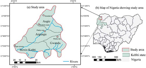
The climate of the area is tropical continental type; with two clear marked seasons, the dry and wet seasons resulting from two contrasting air masses, the tropical continental and tropical maritime originating from the Sahara Desert and the Atlantic Ocean, respectively. The wet season lasts May–October. While the dry season lasts November–April. The mean annual rainfall is 800 mm. The average temperature is 27°C which can rise to 40°C in the summer. Sudan savannah is the predominant vegetation type in the area (Keay 1949). There has been little quantitative analysis of vegetation phenology in this region. More studies are conducted in South African savannah. Since savannah sites are context-dependent, the spatial and temporal analysis of PFTs dynamics in this area is important.

In this study, the major PFTs in the study area were considered, woody and herbaceous components, as well as the cropland (in the upland and Fadama (around the river) land). Most of the previously available land cover (e.g. MODIS reference and GlobCover land cover map reference) do not clearly represent the land cover types in the area. We have used the SPOT (and Google Earth) data (4 May 2005) at 5 m spatial resolution for qualitative evaluation of the sites. Our visual analyses of MODIS land cover product and SPOT data show that a greater proportion of the study area is dominated by agricultural fields. A study by Sedano, Molini, and Azad (2019) indicated that the area is intensely cultivated. Thus, employing the Google Earth, the SPOT data (5 m) and expert knowledge on the local species, the distribution of woody, herbaceous, and dryland crops was identified. Based on these sources, the land cover types were categorized according to the IGBP’s land cover classes. The high-resolution imagery of each location is shown in Figure 2(a,e). The description of the PFTs is given below:

1. Woody cover (thickets): these include dense shrubs and tall trees. These species include Azadirachta indica, Pilliostigma reticulatum, Combretum verticellatum, Guira senegalensis, and Combretum nigricans. The dominant species are the Combretum nigricans and Guira senegalensis. The total size of the area is therefore 75 ha, covering 12 neighbouring pixels of MODIS NDVI data (250 m).

2. Open shrubs: the dominant shrubs are Piliostima thonningii, Guira senegalensis, and Acacia nilotica. The total size of the area is therefore 50 ha, covering 8 neighbouring pixels of MODIS data (250 m x 250 m) (Figure 2(b)).

3. Grassland; the grass community is highly heterogeneous in this area. The grass species are Borroria scabra, Digitaria horizontalis, Pennistum peicellatum, Borroria radata, Corchorus fascicularis Lam (karangiya), Commelina forskalei, Eragrostis gangetica, etc. However, the Pennisetum peicellatum, Corchorus fascicularis Lam and Eragrostis gangetica are not only the dominant species but have more longer growing period than others. In this PFT, the same only 6 pixels of MODIS data of 250 m were covered. This covered only 37.5 ha (Figure 2(c)).

4. Dryland crops: in this region, Pennisetum typhoides (millet), Sorghum bicolour (sorghum), and Vigna unguuiclata (beans) are the main crops being cultivated. The cultivation system is completely rainfed agriculture. Pennisetum typhoides and Vigna unguuiclata are mostly planted under mixed cropping system. Their harvesting period varies because Pennisetum typhoides is usually planted earlier than Vigna unguuiclata. Pennisetum typhoides takes 3 months before it is harvested. The harvest period is normally 7 weeks before the end of rainy season. Vigna unguuiclata is normally harvested towards the end of the rainy season because people use its leaves as hay for animals. Grasses such as Pennisetum peicellatum, Eragrostis gangetica, and Corchorus fascicularis Lam predominantly occupy the cropland area after the harvesting period. In this PFT, nine neighbouring pixels (56.25 ha) of MODIS data were covered. This is one of the most homogenous areas covered by the PFTs under investigation. There were large and extensive farmlands in the area (Figure 2(d)).

5. Paddy rice: Oryza sativa (rice) is mostly cultivated in the rainy and dry season. Lycopersecum esculentum is sometimes cultivated alongside Oryza sativa during the dry season. Note that rainfed agriculture (rice cultivation) also take place during the rainy season which therefore adds up to the total annual NDVI. The area is regularly cultivated because of its proximity to the main river. Only 6 pixels (37.5 ha) of MODIS data (250 m x 250 m) were used for this PFT in order not to include the water bodies.

Figure 2. The locations of the main study sites as extracted from the high-resolution SPOT (m) data at 5 m spatial resolution (4 May 2005) to visualize the PFTs (woody, open shrubs, grassland and dryland crops areas)

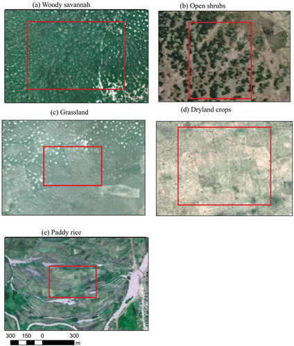
Figure 2: the locations of the main study sites as extracted from the high-resolution SPOT (m) data at 5 m spatial resolution (4 May 2005) to visualize the PFTs (woody, open shrubs, grassland, and dryland crop areas).

2.2. Data

2.2.1. MODIS NDVI time series data

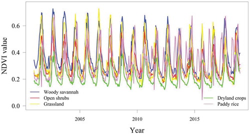
To measure the variation of phenological changes in PFTs, we used MODIS NDVI data, MOD13Q1 product acquired from January 2001 to December 2018 (Didan 2015; DAAC 2019). MOD13Q1 is a gridded level 3 product provided at 250 m spatial resolution every 16 days produced from atmospherically corrected bi-directional surface reflectance factors (BRFs) and masked for water, clouds, and cloud shadows (Strahler et al. 1999; Didan 2015). The data were obtained from the National Aeronautics and Space Administration (NASA) via https://modis.ornl.gov/cgibin/MODIS/global/subset.pl. With 23 images per year, the data set has a total time series of 414 gridded NDVI images for 18 years of remotely sensed observations of vegetation greenness from MODIS. Based on our quality assessments using reliability and vegetation index (VI) quality layers included in the MODIS data, only few points of bad quality were found. MODIS vegetation Index user’s guide provides ranking of the data that describes overall quality: −1 (fill/no data: not processed), 0 (good data: use with confidence), 1 (marginal data: useful, but look at other QA information), 2 (Snow/Ice target covered with snow/ice), 3 (cloudy). The highest number of bad point data was found within the paddy rice (nine bad data points), five points for dryland crops, three each for woody savannah and open shrubs while grassland has only one bad data point. We replaced the bad data for these pixels with the average of the NDVI values of before and after the date of the bad data acquisition. The advantages of using NDVI for change detection are that changes in PFTs may be enhanced by NDVI compared to the spectral values (Cai and Liu 2015; Sedano, Molini, and Azad 2019) and the MODIS NDVI data are less sensitive to the effect of illumination and viewing geometry than individual bands (Los et al. 2005). The MOD13Q1 data product has been used widely for monitoring vegetation dynamics (Zhang et al. 2003), for detecting trend and seasonal changes in satellite image time series (Verbesselt et al. 2010a), for estimating fractional cover of PFTs (Ibrahim et al. 2018) and assessing the impact of soil reflectance variation on woody cover estimation (Ibrahim et al. 2019). Figure 3 shows the MODIS NDVI pixel values averaged for each PFT (2001 to 2018).

Figure 3. Mean MODIS NDVI time series for the studied PFT locations 2001–2018

2.2.2. Precipitation data

In this study, we used the precipitation estimation from remotely sensed information using artificial neural networks (PERSIANN) system at a spatial resolution of 0.04^°, developed by the centre for hydrometeorology and remote Sensing (CHRS) at the University of California (Sorooshian et al. 2000; Nguyen et al. 2019) and is available from 2000 to present (daily, monthly, and annual datasets). The data were developed using the neural network function classification/approximation procedures to compute an estimate of rainfall rate at each pixel of the infrared brightness temperature image provided by geostationary satellites. The monthly (from June to September, 2001 to 2018) raster data were downloaded (for each location of PFT) in GeoTIFF format available at CHRS (https://chrsdata.eng.uci.edu/). These data have been found useful for hazards and flood risk assessments especially in data-scarce areas (Kabenge et al. 2017), characterization and trend analysis of annual rainfall (Sobral et al. 2020). The PERSIANN datasets have been compared with other external datasets and were found to be reasonably accurate (r = 0.94, mean absolute error (mm) = 78.92, RMSE (mm) = 100.44, RMSE (normalized) = 0.07) (Nguyen et al. 2019)

2.3. Methods

2.3.1. Estimating phenological parameters (SOS, EOS, and GSL) for PFTs

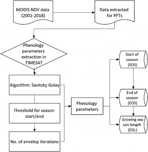
In this study, we extracted phenology parameters using TIMESAT program based on time series of MODIS NDVI for each PFT following recommendations by Jönsson and Eklundh (2004). By using TIMESAT, we estimated the SOS, EOS, and GSL which are of very critical stages of vegetation growth. The time series analysis methods available in TIMESAT software can capture the inter-annual changes, i.e. changes in seasonal timing between years. They reduce the influence of clouds and atmospheric constituents in satellite-derived time series data. It is also possible to process the time series that are unevenly sampled using the time stamp associated with the maximum-value composites.

The TIMESAT program package is specifically designed primarily for analysing time series of satellite data using three methods: Savitzky–Golay filtering, asymmetric Gaussian, and double logistic model functions (Eklundh and Jönsson 2011; Jönsson and Eklundh 2004; Jonsson and Eklundh 2002). Although all these methods were tested and found to a great extent to preserve the integrity of the signals, previous studies found that Savitzky–Golay filtering is not only reliable for the estimation of phenological parameters (e.g. start of growing season) but outperformed other filters (e.g. asymmetric Gaussian, spline smoothing, double logistic fitting) (Lara and Gandini 2016; Cong et al. 2012). In this study, Savitzky–Golay filter was used because of its good performance in modelling the local variation of time series data by preserving the area, position, and peak of the vegetation signals (Jönsson and Eklundh 2004). This makes the algorithm suitable for vegetation dynamics assessments and is applicable to our study area (Heumann et al. 2007). Figure 4 shows the processing steps implemented for the extraction of phenological parameters in TIMESAT.

Figure 4. Flowchart showing the dataset used and the processing procedure for estimating NDVI based phenological parameters of PFTs using TIMESAT and Savitzky–Golay algorithm

2.3.2. Relationships between the SOS or EOS and GSL

Since the ecosystem productivity and surface albedo, for example, can be influenced from the lengthened growing season (Richardson et al. 2013), the relationships between the SOS or EOS and GSL were investigated for each PFT using simple linear regression to evaluate whether SOS or EOS could affect GSL. The significance of the relationship was also assessed at α = 0.05. Data analysis was carried out in R statistical software (R Core Team, 2020).

2.3.3. Estimating annual and interannual variability of PFTs

The annual variability of PFTs was quantitatively compared using the biweekly NDVI time series. The interannual variability of the same PFTs were analysed using the interannual mean NDVI derived from the MODIS data. The SOS, EOS, GSL were also used to assess the interannual variability of the PFTs.

2.3.4 Comparison of phenological metrics between tree phenology and other PFTs using the Welch’s test.

Welch’s t-test was used to determine how well the different PFTs can be distinguished from the woody savannah by using SOS, EOS, GSL mean, and maximum NDVI. The Welch test is a two-sample t-test and does not assume equal variances of the samples (Welch 1938). The Welch test was calculated for each PFT (only open shrubs and grassland in this case) versus the woody phenology.

2.3.4. Breaks For Additive Seasonal and Trend (BFAST)

BFAST is developed mainly to integrate the decomposition of time series into trend, seasonal, and remainder components with methods for detecting change within time series (Verbesselt et al. 2010a, 2010b). BFAST is a generic change detection approach to disentangle a trend component, disturbances (e.g. fires, insect attacks) and a seasonal component which indicate phenological changes. This technique is capable of identifying the PFT successional pathway of phenological development of certain PFT and whether it is strongly affected by the disturbance. (Fang et al. 2018). The number, time, and magnitude of the abrupt changes were assessed for each PFT using the BFAST algorithm. BFAST was developed by Verbesselt et al. (2010a) and has been used successfully to assess the seasonal and abrupt changes within the time series (Verbesselt et al. 2010a; Watts and Laffan 2014; Fang et al. 2018; Geng et al. 2019). BFAST integrates the decomposition of time series into trend, seasonal, and remainder components with methods for detecting breakpoints within time series (Verbesselt et al. 2010a).

The model is characterized by an additive decomposition that iteratively fits a piecewise linear trend and a seasonal model where linear and seasonal components can change at different times, so-called break points. The seasonal component is fixed between seasonal break points, but can vary across break pots and the seasonal break points may be different from the break points of the trend component. (Verbesselt et al. 2010a).

The general model can be expressed in the following equations:

(1) $Y_i\left(t\right)=T_i{\left(t\right)}_{\hspace{0.17em}}+S_i\left(t\right)+e_i\left(t\right),i=1,\dots ,n$(1)

where Y_i(t) is the observed data at time point t_i, T_i(t) is the trend component, S_i(t) is the seasonal component, and e_i(t) is the remainder component, $t_i\le t<t_{i+1},i=0,\dots ,n$-1. The remainder component is the remaining variation in the data beyond that in the seasonal and trend components (Cleveland et al. 1990). It is assumed that T_t is piecewise linear with breakpoints ${\tau }_1$, …, ${\tau }_m$and define${\tau }_0$= 0; therefore, T_j can be expressed by (Verbesselt et al. 2010a)

(2) $T_j\left(t\right)={\alpha }_j+{\beta }_j\left(t\right),j=1,\dots ,m$(2)

where α_j and β_j are the intercept and slope of the linear models, respectively (Verbesselt et al. 2010a). These variables can be used to derive the magnitude and direction of the abrupt change by calculating the difference between T at t_j−1 and t_j as follows:

(3) $Magnitude=({{\alpha }_{j-}}_1{-}_{\hspace{0.17em}}{\alpha }_j)+({{\beta }_{j-}}_1-{\beta }_j)t$(3)

The iterative algorithm to detect breakpoints begins with an estimate of the seasonal component using a seasonal-trend decomposition procedure (Verbesselt et al. 2010b). Then, the following steps are iterated until the number and the position of the breakpoints exhibit no changes: (1) the existence of abrupt changes is assessed by using ordinary least squares (OLS) residuals-based moving sum (MOSUM) test; (2) The trend coefficients, α_j and β_j for j = 1, … , m, are then computed using robust regression of Eq. (3)(3) $Magnitude=({{\alpha }_{j-}}_1{-}_{\hspace{0.17em}}{\alpha }_j)+({{\beta }_{j-}}_1-{\beta }_j)t$(3) based on M-estimation; (3) by using the OLS-MOSUM test, the number and position of the seasonal break points are estimated from the detrended data (4) the seasonal coefficients are computed using a robust regression based on the M-estimation

By using the BFAST Package, all parameters described above were determined automatically except two parameters; (1) the harmonic or dummy model which is used based on vegetation type. Harmonic model is suitable for a natural vegetation while dummy model is recommended for dryland crops (Verbesselt et al. 2010a), in this study, the analyses were carried out following this recommendation; (2) The minimum interval period between the adjacent abrupt changes. Previous studies recommended that the interval period that could be used as the minimum interval between adjacent abrupt changes should be used with caution as it affects the accuracy of the BFAST (Verbesselt et al. 2010a). Large intervals may lead to the omission of certain abrupt changes while short intervals may result in spurious detection of abrupt changes (Verbesselt et al. 2010a). In this study, we used a minimum of 1 year of NDVI data (i.e. 23 observations) between successive change detections (Verbesselt et al. 2010a) but only seasonal abrupt changes of the PFTs were regarded. This is because PFTs (e.g. woody species and grasses) have different phenological cycles (Ibrahim et al. 2018) which means high interval may lead to omission of seasonal abrupt changes in certain PFTs that are more susceptible to seasonal attack (e.g. grasses). On the other hand, based on recommendation by Fang et al. (Fang et al. 2018), we hypothesized that the minimum interval between adjacent significant abrupt changes (in the trend components) was approximately 2 years. Therefore, we set a 2-year interval for detecting the abrupt changes in the trend components.

2.3.6 Assessing the relationship and correlation between the disturbances (breakpoints) estimated using BFAST and precipitation data

In this study, the purpose of correlation analysis was to measure the strength and direction of association between the disturbance and precipitation data as one of the important drivers of vegetation change in the study area. Spearman’s rank correlation coefficient (r) analysis was conducted between the disturbance (breakpoints) which was estimated for each PFT (woody savannah, open shrubs, and grassland), using BFAST algorithm. In addition, coefficient of determination (R²) was also used to assess their relationship. The significance level was assessed at α = 0.05.

3. Results

3.1. The variability of NDVI based phenology for the PFTs over the study period (2001-2018)

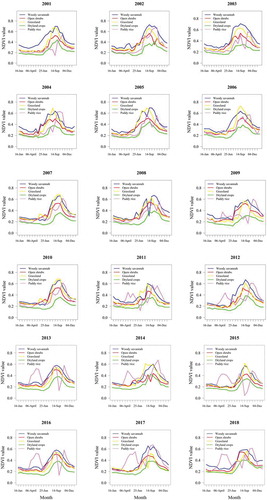
Figure 5 shows the monthly changes of the NDVI from January to December for each PFT for 18 years. As shown here, based on the NDVI phenology, the woody savannah has the highest NDVI during the dry season, except for the period during 2009 to 2018 where the paddy rice is above all PFTs from February to June. In this region, the peak of the growing season for the paddy rice occurs in April. In June, the NDVI-based phenology for all PFTs rises until the peak period of the growing season in September. The woody savannah maintained the highest NDVI throughout the growing season except in a few years where the NDVI phenology for grass and paddy rice overlapped. The grass NDVI phenology is higher than open shrub throughout the growing period for 18 years except on a few occasions during the dry season. The highest monthly rainfall that normally occurs in September is consistent with the maximum NDVI phenology of PFTs occurring in the same month except for the paddy rice where the peak occurs mostly around October/November.

Figure 5. The variability of NDVI based phenology for the PFTs using the averaged NDVI time series data from 2001 to 2018

3.2. The variability of NDVI based phenology in PFTs and its corresponding precipitation data during 2001 to 2018

3.2.1. The variability of NDVI phenology and precipitation total for the PFTs

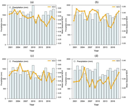
The mean seasonal NDVI phenology of the PFT as well as their corresponding precipitation data is depicted in Figure 6(a, d). The NDVI profiles varied in magnitude and phenology, with the woody phenology showing the highest mean seasonal NDVI throughout the study period except in 2011, 2014, and 2016. The high NDVI phenology of grasses may be connected to early onset of precipitation experienced in those years (Figure 6(a)). Nonetheless, the NDVI-based phenology for the grass is highly variable. The dryland crops had the lowest seasonal mean NDVI because crops are usually cultivated once in a year (in one season) and are usually harvested before the end of rainy season. With reference to CHS precipitation data, we observed that in most PFTs (natural vegetation), the NDVI phenology increases with increasing precipitation. It is however not consistent throughout the period as there are years with the very high precipitation recording very low NDVI. The changes of NDVI phenology in most PFTs do not keep pace with the changes in precipitation in some years. It was observed that grassland is more sensitive to precipitation changes than woody species.

Figure 6. The variability of NDVI based phenology for the PFTs during 2001 to 2018, seasonal mean NDVI with corresponding information from the precipitation data, Woody savannah (a), Open shrubs (b), Grassland (c), Dryland crops (d)

3.2.2. The interannual SOS, EOS and GSL based NDVI phenology for the PFTs during 2001-2018

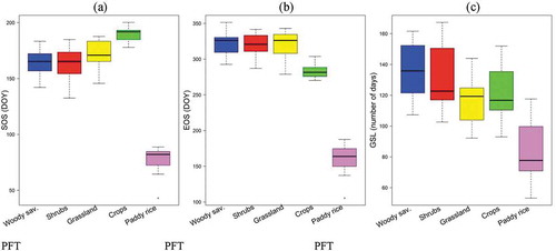
Figure 7 shows the interannual SOS, GSL, and EOS for the PFTs. Paddy rice had the earliest SOS (43 to 88, day of the year (DOY)) compared with all PFTs (Figure 7(a)) even though no growing seasons were detected for 2002 and 2005 for this particular PFT. Irrigational activities usually start in February/March every year. And its GSL is shorter. The longest season for the paddy rice lasts at the 118th DOY (Figure 7(b)). Although the open shrubland had the earliest SOS, compared to all other PFTs, the woody savannah record more years of early SOS compared with other PFTs (Figure 7(a)). The earliest SOS for woody savannah was observed at the 142th day in 2001 and 132th day for open shrubs in 2004. This is followed by grassland and dryland crops. The average period for the SOS of grassland is June (170 DOY) but the earliest is 146th day which was observed in 2005. The phenology of woody savannah had the most prolonged senescence period and invariably observed the longest GSL (Figure 7(b)). Dryland crops had the earliest senescence period which was observed around 290th day of the year. This because most crops take up to 15 weeks before harvest.

Figure 7. The variation of SOS, EOS and GSL based on NDVI phenology of PFTs (2001–2018) estimated with Savitzky–Golay algorithm

3.3. Linear relationships between the SOS or EOS and GSL

In order to assess whether SOS or EOS can determine the GSL, we further analysed the linear relationships between them (Table 1). The SOS for the woody savannah versus GSL shows moderate inverse relationship (R2 = 0.41, p < 0.01) while EOS shows a weak positive relationship (R2 = 0.20, p < 0.06). The relationships for open shrubs indicated a strong inverse relationship (R2 = 0.79, p < 0.001) with the SOS while the EOS of the same PFT shows very weak and insignificant relationship (R2 = 0.20, p < 0.06). With grassland, the relationship between the GSL and SOS or EOS had R2 = 0.35, p < 0.01 and R2 = 0.11, p = 0.17, respectively. The SOS for dryland crops had a weak relationship (R2 = 0.22, p = 0.04) with the GSL while EOS indicated a strong positive relationship (R2 = 0.75, p < 0.001). The relationships between the GSL and SOS or EOS for paddy rice had a very weak inverse (R2 = 0.008, p < 0.73) and strong positive (R2 = 0.69, p < 0.001) relationships, respectively.

Table 1. Linear relationships between the GSL and SOS or EOS for each PFT during 2001–2018

PFTs	SOS vs GSL		EOS vs GSL
	R2	p	R2	p
Woody savannah	0.41	<0.01	0.20	0.06
Open shrubs	0.79	<0.001	0.20	0.06
Grassland	0.35	0.01	0.11	0.17
Dryland crops	0.22	0.04	0.75	<0.001
Paddy rice	0.01	0.73	0.69	<0.001

Overall, linear relationships indicated that the GSL for the less managed vegetation types is mostly determined by the SOS (woody savannah, open shrubs, and grassland) and for the highly managed vegetation types, GSL is being determined by the EOS (dryland crops and paddy rice).

3.4. Comparing the phenological metrics of woody species and other PFTs using the Welch’s test

Table 2 shows the level of associations between the phenological metrics for woody versus open shrubs, and grasses using the Welch’s t-test. The SOS for woody savannah is more associated with open shrub (p = 0.74) than for grasses (p = 0.10). Furthermore, woody savannah phenology shows a distinct GSL. Grassland shows statistically significant difference with the GSL of woody savannah while, for open shrubs, it was insignificant (p = 0.23). The study found a statistically significant difference for all PFTs with mean NDVI of woody phenology (p < 0.001). This could be due to the fact that woody phenology is less prone to interannual variability than other PFTs. For the maximum NDVI, open shrubs show a statistically significant difference (p < 0.001) while it is otherwise with grasses (p = 0.35).

Table 2. Results of Welch two-sample t-tests for woody savannah against other PFTs

Phenological metric	Open shrubs	Grassland
	p value
SOS	0.74	0.10
EOS	< 0.68	<0.80
GSL	0.23	< 0.001
Mean NDVI	< 0.001	< 0.001
Max. NDVI	< 0.001	0.35

3.5. Abrupt changes identified based on NDVI phenology for the PFTs

In the study area, all PFTs except woody species experienced at least one abrupt seasonal change (NDVI increasing, so greening, or NDVI decreasing, so browning) between 2001 and 2018 using a minimum of 1 year of data (i.e. 23 observations) between successive changes in BFAST. Only two abrupt seasonal changes were detected for open shrubs, in 2002 and 2006. Three seasonal changes were found for grasses, in 2004 (greening), 2006 (greening), and 2007 (browning). Grass phenology appeared to be more vulnerable to abrupt changes in seasonal components. Grasses responded more strongly to annual seasonal cycles than woody species. In dryland crops, two seasonal abrupt changes were found, in 2004 and 2005, both greening. Only one seasonal change (greening) was found for paddy rice in the first breakpoint, which occurred in 2011.

Up to five abrupt changes in the trend component of the NDVI time series were determined (Table 3) except for paddy rice (Figure 8(e)). Breakpoints were nearly always negative changes; only in dryland crops and grass, there was one positive change was detected each in 2005 (0.07). In the trend component include shrubs, grasses and dryland crops, especially in the third and fourth breakpoints. Woody phenology had three abrupt negative changes each, one in each breakpoint. The changes occurred in 2004 (−0.0624), 2011 (−0.059) and 2015 (−0.0491). Similarly, three negative magnitude abrupt changes were detected for open shrubs (with negative between −0.089 and −0.064) in 2004, 2011, and 2014, that is, one negative magnitude at each breakpoint.

Table 3. Number of breakpoints and their magnitude (positive (+v) or negative (-v)) based on NDVI phenology for PFT extracted from MODIS time series data (2001–2018) using BFAST. There was only one positive breakpoint but multiple negative ones. No linear breakpoints were found for paddy rice

PFT					Breakpoint abrupt change
	1			2		3			4		5
	Year	+v	-v	Year	-v	Year	-v	Year	-v	Year	-v
Woody savanna	2004	-	−0.062	2011	−0.059	2015	−0.049	-	-	-	-
Open shrubs	2004	-	−0.06	2011	−0.059	2014	−0.081	-	-	-	-
Grassland	2005	0.05	-	2009	−011	2011	−0.095	2015	−0.05	2017	−0.09
Dryland crop	2005	0.07	-	2009	−0.05	2011	−0.02	2015	−0.47	-	-

Figure 8. BFAST decomposition results of the NDVI time series from 2001 to 2018 indicating abrupt magnitudes for woody savannah (a), Shrubland (b), Grassland (c), Dryland crops (d), Paddy rice (e), Yt is the original NDVI data, St, Tt and et stand for decomposed seasonal, trend and remainder components. The small dot line on the graphs show the breakpoint abrupt change

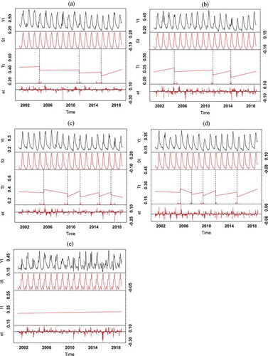
Five abrupt magnitudes were detected for grasses including one abrupt positive change found in 2005 (0.05), while negative magnitudes correspond to break dates in 2009 (−0.11), 2011 (−0.095), 2015 (−0.05) and 2017 (−0.0891). The abrupt browning found for grasses was the largest negative magnitude compared to all PFTs. Here, grass phenology appeared to be more vulnerable to abrupt changes than woody species, seasonally as well as in the trend components with decreasing trend following the abrupt browning (Figure 8(c)). Grasses suffer great disturbances and reflected those effects by responding more strongly to annual changes through the abrupt greening and browning trends.

In dryland crops, there were four abrupt changes in the negative magnitude ranging from −0.06 to −0.03, in 2009 (−0.05), 2011 (−0.02) and 2015 (−0.047). In addition, one positive magnitude change was detected in 2005 (0.07). The changes could be due to harvest, massive clearance of vegetation in preparation for farming or response of crops to drought and harsh weather conditions. However, all negative magnitude for dryland crops as detected from the NDVI time series have an increasing trend following the changes which might suggest vegetation growth probably occurring due to intensification of farming activities following after disturbance. We observed that the phenology of paddy rice (lands) shows high year to year variability compared to other PFTs.

3.6. Relationship and correlation between the vegetation disturbance and precipitation

We assessed the correlation and relationship between vegetation disturbance (assessed using BFAST) and precipitation data from CHRS for PFTs (Table 4). In all PFTs, precipitation data correlate negatively with the disturbance which means that as the precipitation increases the magnitude of disturbance decreases. This is because most of the changes from these PFTs are in the negative magnitude. Only grassland recorded one positive magnitude. In woody species (Savannah and Shrubland), we observed a moderate negative correlation between the precipitation and disturbance (both r = −0.5), while grassland showed a strong negative correlation which means that grass phenology responds more strongly to annual precipitation (r = −0.70) than the woody species. Furthermore, the relationship between the two was assessed using regression analysis. The breakpoint abrupt change for woody species shows very weak and insignificant relationship (woody savannah; R² = 0.05, p = 0.85 and Open shrubs: R² = 0.23, p = 0.67) with precipitation data. For grassland, a moderate positive relationship was observed (R² = 0.59, p = 0.12) (Table 4)

Table 4. Relationship and correlation between vegetation disturbance and precipitation

PFT	Correlation coefficient (r)	R2	p
Woody savannah	−0.5	0.05	0.85
Open shrubs	−0.5	0.23	0.67
Grassland	−0.70	0.59	0.12

4. Discussion

This study investigated whether satellite remote sensing of phenological variability from the MODIS NDVI-based phenology data using Savitzky–Golay filtering and the BFAST algorithm can be applied to detect the variation of PFTs as well as their interannual differences and how they respond to precipitation and disturbances. The variability in the relative compositions of woody and herbaceous vegetation for savannah vegetation, in general, is well documented (Scholes and Archer 1997). The influence of environmental factors (e.g. fire, herbivores, species composition, and precipitation) to annual, seasonal, intra-seasonal, interannual, and spatial changes in plant phenology in savannahs have been reported in the literature (Scholes and Walker 1993; Sankaran et al. 2005). Despite the fact that the NDVI-based phenology of PFTs presents complex phenological pattern in the study area, probably due to species composition and high interannual climate variability – as reflected by fairly large remainder terms, our study demonstrated that phenological changes in PFTs can be distinguished by assessing reference areas with predominant characteristics in a landscape and by using multispectral and multi-temporal remote sensing MODIS NDVI data.

The PFTs investigated present a distinct seasonal, annual and interannual variability (Figure 5, 6(a, c) and 7(a, c)). During the dry season, woody savannah has the highest NDVI, except for the period from 2009 to 2018 where the paddy rice is above all PFTs from February–June (Figure 5). The woody phenology maintained the highest NDVI phenology throughout the growing season except in few years where grass NDVI phenology overlapped. Dryland crops also follow closely rain patterns with higher NDVI during the rainy season (May–October) and low values during the dry season (Figures 5 and 6(a, b)). However, the rainy season NDVI phenology of dryland crops is comparatively lower than those of woody species and grasses (Figs. 5 and 6(a, b)). This resulted possibly due to differences in densities as crops do not commonly cover the ground completely (Sedano, Molini, and Azad 2019). Our results for the seasonal variability of NDVI phenology for PFTs correspond with the annual temporal profile of natural vegetation, dryland crops, and irrigated agriculture as presented for the year 2015 in a recent study (Sedano, Molini, and Azad 2019) whose aim was to develop a mapping framework to characterize land use in the Sudan-Sahel region from dense stacks of Landsat data in Northern Nigeria.

The PFTs show variability in their mean NDVI phenology, SOS (green up), EOS (senescence) and GSL over the study period (Figure 5b, 6a, c). Paddy rice had the earliest greening period occurring throughout the study period. This is because irrigational activities occur in the dry season (January to May) when most PFTs of the natural vegetation were leaf-out. In contrast, the SOS for dryland crops is the later, compared to all PFTs. Woody species were found with the early SOS and their GSL is longer due to their prolonged senescence period. Most woody species retained their greenness until late in the dry season (Figure 5). While grass phenology had late SOS and invariably record a shorter period of GSL compared to woody species (Figure 7). Previous studies reported that ecosystem productivity can be influenced from the lengthened growing season (Richardson et al. 2013; Du et al. 2019), in this study, the relationships between the GSL and SOS or EOS were assessed for all PFTs. We found that GSL is mostly determined by the SOS except in dryland crops and paddy rice. Strong positive relationships were found between the GSL and EOS (R2 = 0.75, p < 0.001 and R2 = 0.69, p < 0.001, Table 4) for dryland crops and paddy rice, respectively. This because crop growth is not only influenced by natural (e.g. weather variability) conditions but is also affected by the field management activities (timing of sowing and harvest). (Richardson et al. 2013; Huang et al. 2019). Detecting crop phenological parameters is very useful for crop growth and health monitoring and yield estimation (Busetto, Zwart, and Boschetti 2019).

Our comparison of SOS, EOS, mean, and maximum NDVI phenology between the woody phenology and other PFTs provides some of the most insightful for differentiating them, which further supported previous studies (local and regional) on the assessments of their differences (Scholes and Walker 1993; Adole, Dash, and Atkinson 2018). Maximum NDVI phenology for woody savannah was not significantly different with grasses (p = 0.35, Table 2). This is possibly as a result of a rapid growth response by grasses following the first rains and subsequent nutrient availability through the decomposition of litter during the dry season in savannah dominated landscapes (de Bie et al. 1998). Likewise, we found no significant differences between the woody species and grass phenology on SOS. A recent study by Adole et al. (Adole, Dash, and Atkinson 2018) showed large-scale pre-rain vegetation green-up across northern and southern Africa, especially for woodland areas.

Using the mean NDVI and GSL phenological parameters, we found a significant difference between woody and grass phenology (p < 0.001). This can be explained by the fact that there are various characteristic differences in the biology of woody species (trees), and grasses. In savannahs, the first greening signal shown by the NDVI data is due to tree leaf flush (Archibald and Scholes 2007). The maximum tree greenness values and tree green-up rates are constant between years (Archibald and Scholes 2007). In savannahs, woody species usually produce new leaves before the first rains as a result of the influence of temperature, moisture, and photoperiod (de Bie et al. 1998). Therefore, woody plants (trees) benefit from being able to grow during the dry season when water is limited and unavailable to grasses (Scholes and Walker 1993). In this study, the dominant woody species are the Guira senegalensis and Combretum nigricans. Based on the classification of main phenological groups of woody plants of the West African savannah dominated landscape the Guira senegalensis is characterized as a semi-evergreen species whilst the Combretum nigricans as the deciduous species being sprouting in the late dry season (de Bie et al. 1998). The mean seasonal precipitation is one of the most important factors determining the spatial patterns of grass abundance in West Africa (Bocksberger et al. 2016; Adole, Dash, and Atkinson 2018). Similarly, large post rains green up were found for crops in the Sudano-Sahelian region (Adole, Dash, and Atkinson 2018). Reasons for these differences are not limited to the leafing of the woody species which pre-empt rainfall (de Bie et al. 1998), but also that woody species have a much longer prolonged senescence period compared to other PFTs. Richardson et al. (2013) explained that far too little attention has been paid to phenological events at the EOS. The phenological events at the EOS play an important role in mediating the feedbacks of vegetation to climate system (Richardson et al. 2013).

The NDVI-based phenology of PFTs assessed in this study varies widely in this region and over time, reflecting the interacting influences of climatic and edaphic conditions (e.g. water limitations on growth), inter-species resource competition, disturbance (e.g. insect attacks and wildfire), herbivory and land use (e.g. grazing and agriculture) (Belsky 1992; Leßmeister et al. 2019). The current study, therefore, investigated the presence of abrupt changes in the NDVI time series and further assessed how PFTs are affected in terms of positive or negative magnitude changes (Figures 8(a, e), 10(a, b), Table 3). No seasonal abrupt change was detected for woody phenology but all PFTs experienced at least one abrupt seasonal change from 2001 to 2018. Only grass phenology has three seasonal abrupt changes in positive and negative magnitudes.

In the trend components, woody species phenology had only three abrupt changes (Figure 8a, b). And it takes woody species an interval of four to 8 years between the successive abrupt browning trends. In addition, greening trends were observed following the abrupt changes. The changes in woody species phenology are of very less negative magnitude (Table 3). In contrast, five abrupt magnitudes were detected for grasses including one abrupt positive change (Figure 8(c)). The abrupt browning found for grasses was the largest negative magnitude compared to all PFTs. It takes an interval of exactly 4 years between the first abrupt greening and only 2 years interval between the successive abrupt browning for grass phenology. The interval between the abrupt phenological changes is, therefore, shorter for grass phenology. In 2018, a browning trend was observed in grass phenology despite the occurrence of an abrupt browning trend in 2017. This is not unexpected considering that grass phenology has a longer recovery period following disturbance. In all PFTs, breakpoint (disturbance) assessed using BFAST negatively correlate with precipitation data which means the magnitude of disturbance decreases with increasing precipitation (Table 4). Woody species had an r value of −0.5 while grassland had r = −0.7 which is a further indication that grass phenology responds more strongly to annual precipitation than the woody species. Woody species (especially trees) usually have well-developed roots, which enable them to extract groundwater. They are less dependent on rainfall than the shallow-rooting grasses, which rely on short-lived rainfall. They are also more resistant to fire and can recover more easily after a fire once they have grown to a certain height and escaped the ‘fire trap’ (Ibrahim et al. 2018; de Bie et al. 1998). A recent study by Leßmeister et al. (2019) who studied vegetation changes over the past two decades in a West African savannah ecosystem found no change in woody species composition and richness over the past two decade studies while grass species have changed and species richness has increased.

No phenological changes are detected in the paddy rice when the assumption of 2 years was used as the minimal segment sizes between potentially detected breaks (Figure 9(b)) whereas phenological changes are always detected in other PFTs using the same assumption. This is possibly because the detection of phenological changes is influenced by the signal-to-noise ratio of the NDVI time series. Previous studies have emphasized on potential difficulties in using BFAST to monitor plantations (Fang et al. 2018; Geng et al. 2019). Having found no abrupt changes in paddy rice, especially in the trend component, on the contrary, a minimum of 1 year of data (i.e. 23 observations) between successive change detections were proposed as the interval between adjacent significant abrupt changes and a few abrupt changes were detected (Figure 9(a)).

Figure 9. BFAST decomposition results of the NDVI time series from 2001 to 2018 indicating abrupt magnitudes for paddy rice using different minimal segment sizes between potentially detected breaks (a) minimum of one year of data (i.e. 23 observations), (b) minimum of two year of data (i.e. 46 observations) between successive change detections. Yt is the original NDVI data, St, Tt and et stand for decomposed seasonal, trend and remainder components. The small dot line on the graphs show the breakpoint abrupt change

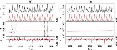
Even though the BFAST algorithms did not capture the agricultural transformation very well, significant changes in the annual NDVI profile for paddy rice can be observed in April from 2009 to 2018 (Figure 5). The month of April is usually the peak of the growing season for irrigated agriculture. In 2015, the anchor borrower Programme policy has been launched by the federal government of Nigeria, mainly to boost agricultural production, by providing, for example, subsidy and loans to farmers. The programme is presently making a positive impact especially to the people of Kebbi state. The greatest agricultural revolution in the study area started in 2016 when agricultural commodity importation was reduced and local farmers were assisted through the anchor borrower programme (Saheed et al. 2018). The BFAST model well captured the upward greening trend in 2016 (Figure 8(a)). In 2017, there was an abrupt browning trend which was as a result of low agricultural production owing to abrupt hike in the price of petroleum product from N86.50 k to N145 per litre and up N250 in the parallel market due change in oil subsidy policy. Many farmers found it difficult to afford to fuel their generators for irrigational activities. Irrigation activities are now being encouraged subsequently and the BFAST algorithm has captured the most recent greening trend as an evidence of an increased agricultural production in the area (Figure 9(a)).

5. Conclusions

In this study, the application of satellite remote sensing in modelling the phenological variability of PFTs over West African savannah dominated landscape was investigated by analysing the MODIS NDVI time series data. The main findings were given as follows:

1. The phenology indicators of the different PFTs present distinct seasonal, annual, and interannual variability. The green up for woody species started earlier than grasses before the rainy season. Grassland responds more strongly to annual precipitation. Dryland crops also follow closely rain patterns with higher NDVI values during the rainy season (May–October) and low values during the dry season.

2. The phenology of woody species has the longest GSL compared to other PFTs and mostly determined by SOS (R2 = 0.41, p = 0.01 and R2 = 0.79, p < 0.001 for woody and open shrubs, respectively). Unlike the woody species, the dryland crops and paddy rice SOS were mostly determined by EOS (R2 = 0.75, p < 0.001 and R2 = 0.69, p < 0.001, respectively) due to possible field management activities.

3. The abrupt vegetation changes estimated varied by PFT. Some PFTs are more resilient to harsh environmental conditions than others. While woody species present a few abrupt changes, grass phenology is more vulnerable to disturbance, seasonally as well as in the trend components (large number of abrupt changes) with browning trend following abrupt negative changes.

4. Our studies detected agricultural changes that were influenced by government policies and programmes geared towards achieving self-sufficiency in basic food supply and job creation in this region.

5. Our studies are limited to the assessment of phenological variability of PFTs at site (with predominant PFT) level and attempted to differentiate them on the basis of their phenological events. More effort should, therefore, go into defining a larger spatial scale to assess this variability from site to regional levels.

6. More studies on phenological variability of PFTs will enhance management strategies to maintain ecosystem function and services, biodiversity and livelihoods in savannah dominated landscape.

Acknowledgements

This work was supported by TETFUND. H. Balzter was supported by the Royal Society, Wolfson Research Merit Award, 2011/R3 and the Natural Environment Research Council (NERC) through the National Centre for Earth Observation (NCEO). We also acknowledge the R Core team for making various library packages available for the data analyses. Special thanks to National Aeronautics and Space Administration (NASA) for providing the MODIS data.

Disclosure statement

The authors declare no conflict of interest.

Additional information

Funding

This research was funded by the Tertiary Education Trust Fund (TETFUND), Nigeria, through the Institution-Based Research Fund (IBRF);Tertiary Education Trust Fund (TETFUND), Nigeria [Institution-Based Research Fund (IBRF).];

References

- Adelana, P. I., R. B. Olasehinde, B. P. Vrbka, A. E. Edet, and I. B. Goni. 2008. “An Overview of the Geology and Hydrogeology of Nigeria.” In Applied Groundwater Studies in Africa, edited by A. MacDonald and S. Adelana, 28. London: CRC Press.
- Adole, T., J. Dash, and P. M. Atkinson. 2018. “Large-scale Prerain Vegetation Green-up across Africa.” Global Change Biology 24 (9): 4054–4068. doi:10.1111/gcb.14310.
- Andrew, M. E., and H. Warrener. 2017. “Detecting Microrefugia in Semi-arid Landscapes from Remotely Sensed Vegetation Dynamics.” Remote Sensing of Environment 200: 114–124. doi:10.1016/j.rse.2017.08.005.
- Archibald, S., and R. J. Scholes. 2007. “Leaf Green-up in a Semi-arid African Savanna -separating Tree and Grass Responses to Environmental Cues.” Journal of Vegetation Science 18 (4): 583–594. doi:10.1111/j.1654-1103.2007.tb02572.x.
- Asner, G. P., and R. E. Martin. 2009. “Airborne Spectranomics: Mapping Canopy Chemical and Taxonomic Diversity in Tropical Forests.” Frontiers in Ecology and the Environment 7 (5): 269–276. doi:10.1890/070152.
- Balzter, H., F. Gerard, C. George, G. Weedon, W. Grey, B. Combal, E. Bartholomé, S. Bartalev, and S. Los. 2007. “Coupling of Vegetation Growing Season Anomalies and Fire Activity with Hemispheric and Regional-Scale Climate Patterns in Central and East Siberia.” Journal of Climate 20 (15): 3713–3729. doi:10.1175/jcli4226.
- Belsky, A. J. 1992. “Effects of Grazing, Competition, Disturbance and Fire on Species Composition and Diversity in Grassland Communities.” Journal of Vegetation Science 3 (2): 187–200. doi:10.2307/3235679.
- Bocksberger, G., J. Schnitzler, C. Chatelain, P. Daget, T. Janssen, M. Schmidt, A. Thiombiano, and G. Zizka. 2016. “Climate and the Distribution of Grasses in West Africa.” Journal of Vegetation Science 27 (2): 306–317. doi:10.1111/jvs.12360.
- Busetto, L., S. J. Zwart, and M. Boschetti. 2019. “Analysing Spatial–temporal Changes in Rice Cultivation Practices in the Senegal River Valley Using MODIS Time-series and the PhenoRice Algorithm.” International Journal of Applied Earth Observation and Geoinformation 75: 15–28. doi:10.1016/j.jag.2018.09.016.
- Cai, S., and D. Liu. 2015. “Detecting Change Dates from Dense Satellite Time Series Using a Sub-Annual Change Detection Algorithm.” Remote Sensing 7: 7. doi:10.3390/rs70708705.
- Cao, X., Y. Liu, Q. Liu, X. Cui, X. Chen, and J. Chen. 2018. “Estimating the Age and Population Structure of Encroaching Shrubs in Arid/semiarid Grasslands Using High Spatial Resolution Remote Sensing Imagery.” Remote Sensing of Environment 216: 572–585. doi:10.1016/j.rse.2018.07.025.
- Cho, M. A., G. P. Renaud Mathieu, L. N. Asner, J. van Aardt, A. Ramoelo, P. Debba, et al. 2012. “Mapping Tree Species Composition in South African Savannas Using an Integrated Airborne Spectral and LiDAR System.” Remote Sensing of Environment 125: 214–226. doi:http://dx.doi.10.1016/j.rse.2012.07.010.
- Cleveland, R. B., W. S. Cleveland, M. Jean E, and I. Terpenning. 1990. “STL: A Seasonal-trend Decomposition Procedure Based on Loess.” Journal of Official Statistics 6 (1): 3–73.
- Cong, N., S. Piao, A. Chen, X. Wang, X. Lin, S. Chen, S. Han, G. Zhou, and X. Zhang. 2012. “Spring Vegetation Green-up Date in China Inferred from SPOT NDVI Data: A Multiple Model Analysis.” Agricultural and Forest Meteorology 165: 104–113. doi:10.1016/j.agrformet.2012.06.009.
- DAAC, O. R. N. L. “MODIS and VIIRS Land Products Global Subsetting and Visualization Tool. ORNL DAAC.” Accessed January 21, 2019. https://doi.org/10.3334/ORNLDAAC/1379
- de Beurs, K. M., and G. M. Henebry. 2010. “Spatio-temporal Statistical Methods for Modelling Land Surface Phenology.” In Phenological Research, edited by Hudson I., Keatley M., 177–208. Springer. https://doi.org/10.1007/978-90-481-3335-2_9
- de Bie, S., P. Ketner, M. Paasse, and C. Geerling. 1998. “Woody Plant Phenology in the West Africa Savanna.” Journal of Biogeography 25 (5): 883–900.
- Didan, K. 2015. “MOD13Q1 MODIS/Terra Vegetation Indices 16-Day L3 Global 250m SIN Grid V006. NASA EOSDIS Land Processes DAAC.” In.
- Du, Q., H. Liu, L. Yaohui, X. LuJun, and S. Diloksumpun. 2019. “The Effect of Phenology on the Carbon Exchange Process in Grassland and Maize Cropland Ecosystems across a Semiarid Area of China.” Science of the Total Environment 695: 133868. doi:10.1016/j.scitotenv.2019.133868.
- Edward, G. P., R. Alfredo Huete, L. Pamela Nagler, and G. Stephen Nelson. 2008. “Relationship between Remotely-sensed Vegetation Indices, Canopy Attributes and Plant Physiological Processes: What Vegetation Indices Can and Cannot Tell Us about the Landscape.” Sensors 8: 4. doi:10.3390/s8042136.
- Eklundh, L., and P. Jönsson. 2011. “TIMESAT3.1 Software Manual.” In.
- Fang, X., Q. Zhu, L. Ren, H. Chen, K. Wang, and C. Peng. 2018. “Large-scale Detection of Vegetation Dynamics and Their Potential Drivers Using MODIS Images and BFAST: A Case Study in Quebec, Canada.” Remote Sensing of Environment 206: 391–402. doi:10.1016/j.rse.2017.11.017.
- Fensham, R. J., R. J. Fairfax, and S. R. Archer. 2005. “Rainfall, Land Use and Woody Vegetation Cover Change in Semi-arid Australian Savanna.” Journal of Ecology 93 (3): 596–606. doi:10.1111/j.1365-2745.2005.00998.x.
- Geng, L., T. Che, X. Wang, and H. Wang. 2019. “Detecting Spatiotemporal Changes in Vegetation with the BFAST Model in the Qilian Mountain Region during 2000–2017.” Remote Sensing 11 (2): 103. doi:10.3390/rs11020103.
- Gitay, H., and I. R. Nobel. 1997. “What are Functional Types and How Should We Seek Them? .” In Plant Functional Types. Their Relevance to Ecosystem Properties and Global Change., edited by H. H. Shugart, T. M. Smith, and F. I. Woodward, 3–19. New York, NY, USA: Cambridge University Press.
- Helmut, L. 1975. “Phenology and Seasonality Modeling.” Soil Sc 120: 461.
- Heumann, B. W., J. W. Seaquist, L. Eklundh, and P. Jönsson. 2007. “AVHRR Derived Phenological Change in the Sahel and Soudan, Africa, 1982–2005.” Remote Sensing of Environment 108 (4): 385–392. doi:10.1016/j.rse.2006.11.025.
- Higgins, S. I., M. D. Delgado‐Cartay, E. C. February, and H. J. Combrink. 2011. “Is There a Temporal Niche Separation in the Leaf Phenology of Savanna Trees and Grasses?” Journal of Biogeography 38 (11): 2165–2175.
- Hill, M. J., M. O. Román, C. B. Schaaf, L. Hutley, C. Brannstrom, A. Etter, and N. P. Hanan. 2011. “Characterizing Vegetation Cover in Global Savannas with an Annual Foliage Clumping Index Derived from the MODIS BRDF Product.” Remote Sensing of Environment 115 (8): 2008–2024.
- Hill, M. J., and N. P. Hanan. 2010. “Ecosystem Function in SavannasMeasurement and Modeling at Landscape to Global Scales.” In. Boca Raton: CRC Press.
- Huang, X., J. Liu, W. Zhu, C. Atzberger, and Q. Liu. 2019. “The Optimal Threshold and Vegetation Index Time Series for Retrieving Crop Phenology Based on a Modified Dynamic Threshold Method.” Remote Sensing 11: 23. doi:10.3390/rs11232725.
- Huete, A., K. Didan, T. Miura, E. P. Rodriguez, X. Gao, and L. G. Ferreira. 2002. “Overview of the Radiometric and Biophysical Performance of the MODIS Vegetation Indices.” Remote Sensing of Environment 83 (1): 195–213. doi:10.1016/S0034-4257(02)00096-2.
- Ibrahim, S. 2013. “Comparing Alternative Methods of Measuring Geographic Access to Health Services: An Assessment of People’s Access to Specialist Hospital in Kebbi State.” Academic Journal of Interdisciplinary Studies 2 (12): 109.
- Ibrahim, S., H. Balzter, K. Tansey, N. Tsutsumida, and R. Mathieu. 2018. “Estimating Fractional Cover of Plant Functional Types in African Savannah from Harmonic Analysis of MODIS Time-series Data.” International Journal of Remote Sensing 39 (9): 2718–2745. doi:10.1080/01431161.2018.1430914.
- Ibrahim, S., H. Balzter, K. Tansey, R. Mathieu, and N. Tsutsumida. 2019. “Impact of Soil Reflectance Variation Correction on Woody Cover Estimation in Kruger National Park Using MODIS Data.” Remote Sensing 11: 8. doi:10.3390/rs11080898.
- Ibrahim, S., I. Hamisu, and U. Lawal. 2015. “Spatial Pattern of Tuberculosis Prevalence in Nigeria: A Comparative Analysis of Spatial Autocorrelation Indices.” Am J Geogr Infor System 4 (3): 87–94. doi:10.5923/j.ajgis.20150403.01.
- Ibrahim, Y. Z., H. Balzter, and J. Kaduk. 2018. “Land Degradation Continues despite Greening in the Nigeria-Niger Border Region.” Global Ecology and Conservation 16: e00505. doi:10.1016/j.gecco.2018.e00505.
- Ilangakoon, N. T., N. F. Glenn, T. H. Hamid Dashti, P. T. Dylan Mikesell, L. P. Spaete, J. J. Mitchell, and K. Shannon. 2018. “Constraining Plant Functional Types in a Semi-arid Ecosystem with Waveform Lidar.” Remote Sensing of Environment 209: 497–509. doi:10.1016/j.rse.2018.02.070.
- Jacques, D. C., L. Kergoat, P. Hiernaux, E. Mougin, and P. Defourny. 2014. “Monitoring Dry Vegetation Masses in Semi-arid Areas with MODIS SWIR Bands.” Remote Sensing of Environment 153: 40–49. doi:10.1016/j.rse.2014.07.027.
- Jetz, W., J. Cavender-Bares, R. Pavlick, F. W. 2016. “Monitoring Plant Functional Diversity from Space.” Nature Plants 2:16024. doi: 10.1038/nplants.2016.24. https://www.nature.com/articles/nplants201624#supplementary-information
- Jonsson, P., and L. Eklundh. 2002. “Seasonality Extraction by Function Fitting to Time-series of Satellite Sensor Data.” IEEE Transactions on Geoscience and Remote Sensing 40 (8): 1824–1832. doi:10.1109/tgrs.2002.802519.
- Jönsson, P., and L. Eklundh. 2004. “TIMESAT—a Program for Analyzing Time-series of Satellite Sensor Data.” Computers & Geosciences 30 (8): 833–845. doi:10.1016/j.cageo.2004.05.006.
- Julius, A. Y., T. Lara Prihodko, W. Armel Kaptué, C. Ross, J. S. Wenjie, S. Kumar, A. Brianna Lind, A. Mamadou Sarr, A. Diouf, and P. Niall Hanan. 2019. “Trends in Woody and Herbaceous Vegetation in the Savannas of West Africa.” Remote Sensing 11: 5. doi:10.3390/rs11050576.
- Kabenge, M., J. Elaru, H. Wang, and L. Fengting. 2017. “Characterizing Flood Hazard Risk in Data-scarce Areas, Using a Remote Sensing and GIS-based Flood Hazard Index.” Natural Hazards 89 (3): 1369–1387. doi:10.1007/s11069-017-3024-y.
- Kattenborn, T., F. E. Fassnacht, and S. Schmidtlein. 2019. “Differentiating Plant Functional Types Using Reflectance: Which Traits Make the Difference?” Remote Sensing in Ecology and Conservation 5 (1): 5–19. doi:10.1002/rse2.86.
- Keay, R. W. J. 1949. “An Example of Sudan Zone Vegetation in Nigeria.” Journal of Ecology 37 (2): 335–364. doi:10.2307/2256612.
- Lara, B., and M. Gandini. 2016. “Assessing the Performance of Smoothing Functions to Estimate Land Surface Phenology on Temperate Grassland.” International Journal of Remote Sensing 37 (8): 1801–1813. doi:10.1080/2150704x.2016.1168945.
- Leßmeister, A., M. Bernhardt‐Römermann, K. Schumann, A. Thiombiano, R. Wittig, K. Hahn, and J. Ewald. 2019. “Vegetation Changes over the past Two Decades in a West African Savanna Ecosystem.” Applied Vegetation Science. doi:10.1111/avsc.12428.
- Los, S. O., P. R. J. North, W. M. F. Grey, and M. J. Barnsley. 2005. “A Method to Convert AVHRR Normalized Difference Vegetation Index Time Series to A Standard Viewing and Illumination Geometry.” Remote Sensing of Environment 99 (4): 400–411.
- Ma, X., A. Huete, Y. Qiang, N. R. Coupe, K. Davies, M. Broich, P. Ratana, et al. 2013. “Spatial Patterns and Temporal Dynamics in Savanna Vegetation Phenology across the North Australian Tropical Transect.” Remote Sensing of Environment 139 :97–115. doi:10.1016/j.rse.2013.07.030.
- Martínez, B., and M. A. Gilabert. 2009. “Vegetation Dynamics from NDVI Time Series Analysis Using the Wavelet Transform.” Remote Sensing of Environment 113 (9): 1823–1842. doi:10.1016/j.rse.2009.04.016.
- Moreno-de Las Heras, M., R. Díaz-Sierra, L. Turnbull, and J. Wainwright. 2015. “Assessing Vegetation Structure and ANPP Dynamics in a Grassland-shrubland Chihuahuan Ecotone Using NDVI-rainfall Relationships.” Biogeosciences Discussions 12 (1): 51–92.
- Nguyen, L. H., D. R. Joshi, D. E. Clay, and G. M. Henebry. 2018. “Characterizing Land Cover/land Use from Multiple Years of Landsat and MODIS Time Series: A Novel Approach Using Land Surface Phenology Modeling and Random Forest Classifier.” Remote Sensing of Environment. doi:10.1016/j.rse.2018.12.016.
- Nguyen, P., E. J. Shearer, H. Tran, M. Ombadi, N. Hayatbini, T. Palacios, P. Huynh, et al. 2019. “The CHRS Data Portal, an Easily Accessible Public Repository for PERSIANN Global Satellite Precipitation Data.” Scientific Data 6 (1): 180296. doi:10.1038/sdata.2018.296.
- Osborne, C. P., T. Charles-Dominique, W. J. Nicola Stevens, G. M. Bond, and E. R. L. Caroline. 2018. “Human Impacts in African Savannas are Mediated by Plant Functional Traits.” New Phytologist 220 (1): 10–24. doi:10.1111/nph.15236.
- R Core Team. 2020. “R: A Language and Environment for Statistical Computing.” Vienna, Austria. Available at: https://www.R-project.org/
- Rapinel, S. 2019. “Evaluation of Sentinel-2 Time-series for Mapping Floodplain Grassland Plant Communities.” Remote Sensing of Environment 223: 115-29-2019 v.223. doi:10.1016/j.rse.2019.01.018.
- Richardson, A. D., T. F. Keenan, M. Migliavacca, Y. Ryu, O. Sonnentag, and M. Toomey. 2013. “Climate Change, Phenology, and Phenological Control of Vegetation Feedbacks to the Climate System.” Agricultural and Forest Meteorology 169: 156–173. doi:10.1016/j.agrformet.2012.09.012.
- Roy, D. P., and L. Yan. 2018. “Robust Landsat-based Crop Time Series Modelling.” Remote Sensing of Environment. doi:10.1016/j.rse.2018.06.038.
- Saheed, Z. S., A. A. Alexander, A. A. Isa, and O. A. Adeneye. 2018. “Anchor Borrower Programme on Agricultural Commodity Price and Employment Generation in Kebbi State, Nigeria.” European Scientific Journal 14: 13.
- Sankaran, M., N. P. Hanan, R. J. Scholes, J. Ratnam, D. J. Augustine, B. S. Cade, J. Gignoux, S. I. Higgins, X. Le Roux, and F. Ludwig. 2005. “Determinants of Woody Cover in African Savannas.” Nature 438 (7069): 846–849.
- Scholes, R. J. 2003. “Convex Relationships in Ecosystems Containing Mixtures of Trees and Grass.” Environmental and Resource Economics 26: 559–574.
- Scholes, R. J., and B. H. Walker. 1993. An African Savanna: Synthesis of the Nylsvley Study, Cambridge Studies in Applied Ecology and Resource Management. Cambridge: Cambridge University Press.
- Scholes, R. J., and S. R. Archer. 1997. “Tree-grass Interactions in Savannas.” Annual Review of Ecology and Systematics 28 (1): 517–544.
- Sedano, F., V. Molini, and A. M. Azad. 2019. “A Mapping Framework to Characterize Land Use in the Sudan-Sahel Region from Dense Stacks of Landsat Data.” Remote Sensing 11: 6. doi:10.3390/rs11060648.
- Sobral, B. S., J. F. de Oliveira-júnior, F. Alecrim, G. Gois, J. G. Muniz-Júnior, P. M. de Bodas Terassi, E. R. Pereira-Júnior, G. Bastos Lyra, and M. Zeri. 2020. “PERSIANN-CDR Based Characterization and Trend Analysis of Annual Rainfall in Rio De Janeiro State, Brazil.” Atmospheric Research 238: 104873. doi:10.1016/j.atmosres.2020.104873.
- Sorooshian, S., K.-L. Hsu, H. V. Xiaogang Gao, B. I. Gupta, and D. Braithwaite. 2000. “Evaluation of PERSIANN System Satellite-Based Estimates of Tropical Rainfall.” Bulletin of the American Meteorological Society 81 (9): 2035–2046. doi:10.1175/1520-0477(2000)081<2035:eopsse>2.3.co;2.
- Strahler, A. H., J. P. Muller, W. Lucht, C. Schaaf, T. Tsang, F. Gao, X. Li, P. Lewis, and M. J. Barnsley. 1999. “MODIS BRDF/albedo Product: Algorithm Theoretical Basis Document Version 5.0.” MODIS Documentation 23 (4): 42–47.
- Tansey, K., J.-M. Grégoire, D. Stroppiana, A. Sousa, J. M. João Silva, C. Pereira, L. Boschetti, et al. 2004. “VEGETATION Burning in the Year 2000: Global Burned Area Estimates from SPOT VEGETATION Data.” Journal of Geophysical Research: Atmospheres 109 :D14. doi:10.1029/2003jd003598.
- Tansey, K., J.-M. Grégoire, P. Defourny, R. Leigh, J.-F. Pekel, E. van Bogaert, and B. Etienne. 2008. “A New, Global, Multi-annual (2000–2007) Burnt Area Product at 1 Km Resolution.” Geophysical Research Letters 35: 1. doi:10.1029/2007gl031567.
- Tucker, C. J., J. R. G. Townshend, and T. E. Goff. 1985. “African Land-Cover Classification Using Satellite Data.” Science 227 (4685): 369. doi:10.1126/science.227.4685.369.
- Ustin, S. L., and J. A. Gamon. 2010. “Remote Sensing of Plant Functional Types.” New Phytologist 186 (4): 795–816. doi:10.1111/j.1469-8137.2010.03284.x.
- Valentini, R., M. Henry, R. A. Houghton, M. Jung, W. L. Kutsch, Y. Malhi, E. Mayorga, et al. 2014. “A Full Greenhouse Gases Budget of Africa: Synthesis, Uncertainties, and Vulnerabilities.” Biogeosciences 11 (2): 381–407. doi:10.5194/bg-11-381-2014.
- Verbesselt, J., R. Hyndman, A. Zeileis, and D. Culvenor. 2010b. “Phenological Change Detection while Accounting for Abrupt and Gradual Trends in Satellite Image Time Series.” Remote Sensing of Environment 114 (12): 2970–2980. doi:10.1016/j.rse.2010.08.003.
- Verbesselt, J., R. Hyndman, G. Newnham, and D. Culvenor. 2010a. “Detecting Trend and Seasonal Changes in Satellite Image Time Series.” Remote Sensing of Environment 114 (1): 106–115. doi:10.1016/j.rse.2009.08.014.
- Vladimir, W. R., R. Stuart Phinn, N. Kuhn, L. Bloemertz, and L. Kiran Dhanjal-Adams. 2016. “Mapping Decadal Land Cover Changes in the Woodlands of North Eastern Namibia from 1975 to 2014 Using the Landsat Satellite Archived Data.” Remote Sensing 8: 8. doi:10.3390/rs8080681.
- Watts, L. M., and S. W. Laffan. 2014. “Effectiveness of the BFAST Algorithm for Detecting Vegetation Response Patterns in a Semi-arid Region.” Remote Sensing of Environment 154: 234–245. doi:10.1016/j.rse.2014.08.023.
- Welch, B. L. 1938. “The Significance of the Difference between Two Means When the Population Variances are Unequal.” Biometrika 29 (3/4): 350–362. doi:10.2307/2332010.
- Whitecross, M. A., E. T. F. Witkowski, and S. Archibald. 2016. “No Two are the Same: Assessing Variability in Broad-leaved Savanna Tree Phenology, with Watering, from 2012 to 2014 at Nylsvley, South Africa.” South African Journal of Botany 105: 123–132. doi:10.1016/j.sajb.2016.03.016.
- Williams, C. A., N. P. Hanan, J. C. Neff, R. J. Scholes, J. A. Berry, A. Scott Denning, and D. F. Baker. 2007. “Africa and the Global Carbon Cycle.” Carbon Balance and Management 2 (1): 3. doi:10.1186/1750-0680-2-3.
- Woodcock, C. E., T. R. Loveland, M. Herold, and M. E. Bauer. 2019. “Transitioning from Change Detection to Monitoring with Remote Sensing: A Paradigm Shift.” Remote Sensing of Environment 111558. doi:10.1016/j.rse.2019.111558.
- Yang, Y., M. Anderson, F. Gao, C. Hain, A. Noormets, G. Sun, R. Wynne, V. Thomas, and L. Sun. 2018. “Investigating Impacts of Drought and Disturbance on Evapotranspiration over a Forested Landscape in North Carolina, USA Using High Spatiotemporal Resolution Remotely Sensed Data.” Remote Sensing of Environment. doi:10.1016/j.rse.2018.12.017.
- Zhang, X., M. A. Friedl, C. B. Schaaf, A. H. Strahler, C. F. John, F. G. Hodges, B. C. Reed, and A. Huete. 2003. “Monitoring Vegetation Phenology Using MODIS.” Remote Sensing of Environment 84 (3): 471–475. doi:10.1016/S0034-4257(02)00135-9.