Extracting three-dimensional (3D) spatial information from sequential oblique unmanned aerial system (UAS) imagery for digital surface modeling

ABSTRACT

The advent of unmanned aerial system (UAS) has prompted close-range imagery a prevalent source to diversify spatial applications. In addition to nadir scenes, UAS is able to take oblique imagery, which increases the opportunity to acquire sophisticated spatial information from different viewing angles. These images provide more possibilities to reconstruct the land surfaces more completely in three-dimensions (3D). However, dealing with UAS imagery for 3D modelling has been a challenging task for years due to unstable and/or unknown exterior orientation parameters (EOPs) measured by direct georeferencing. With sequential oblique UAS imagery with inadequate or missing EOPs, this paper attempts to extract 3D spatial information from these types of images to achieve digital surface reconstruction. A modular workflow integrating the recovery of camera EOPs and 3D reconstruction in a relative space is presented. These images are spatially related by a feature-based incremental structure-from-motion (fi-SfM) for localization, stereo pairs selection and modification. Digital surface reconstruction, thenceforth, is addressed through dense matching and space intersection upon the outcomes of fi-SfM. The experimental results show that the designed schema is coherent in estimating the camera EOPs and modifying the inappropriate image pairs for improved 3D reconstruction. Furthermore, the surface model generated by discrete stereo pairs can be merged automatically to present a complete digital surface model (DSM). The completeness assessment has verified that the majority of the land surface can be successfully obtained by more than 90%, and the accuracy less than 1 (m) indicates that the implemented workflow can be used to achieve 3D modelling effectively.

1. Introduction

The use of unmanned aerial system (UAS), commonly known as drones, in acquiring spatial data has risen in the past decades due to its low economic cost and high degree of flexibility. UAS imagery has been used in various applications across wide-ranging topics, such as three-dimensional (3D) reconstruction and modelling (Aicardi et al. 2016; Pan et al. 2019), urban change detection (Qin 2014), mobile 3D mapping (Siebert and Teizer 2014) and post-hazard supervision and analysis (Aicardi et al. 2016; Al-Rawabdeh et al. 2016). Among these applications, digital 3D modelling brings modern impact on spatial data processing and interpretation by providing an overview of the land surface. Aside from the nadir imagery, one of the most emphasized capabilities of UAS is capturing imagery from different viewing angles. With these UAS oblique imagery, 3D model reconstruction has been more comprehensive for spatial applications and analyses. Take hazard assessment and decision-support service (Mahler, Varanda, and de Oliveira 2012) for example, UAS can capture firsthand images soon after a disaster takes place, providing the spatial data for environmental analyses. Based on these merits, this platform continues its popularity on the aspects of resilient data collection, moderate cost balance (Jiang and Jiang 2018) as well as the potential to support diversified applications.

In terms of optical imagery processing, the fields of photogrammetry (Colomina and Molina 2014; Wolf, Dewitt, and Wilkinson 2014) and computer vision (Carrivick, Smith, and Quicey 2016; Szeliski 2010) have devised their pertinent algorithms. They hold the physical model of centre-perspective projection to describe the spatial linkage between two-dimensional (2D) image and 3D real world. Three staples consisting of exterior orientation parameters (EOPs), 2D image feature and 3D object point play the role of spatial processing in both domains (Szeliski 2010; Wolf, Dewitt, and Wilkinson 2014). With the interior orientation parameters (IOPs) defining the position of the perspective centre relative to the image coordinate system, a pinhole camera model portrays 2D-3D spatial associations. The general question to resolve is the acquisition of 3D object points or the digital surface modelling (Carrivick, Smith, and Quicey 2016; Nex, Rupnik, and Remondino 2013; Rupnik, Nex, and Remondino 2014). Although these two communities hold the similar foundation, they interpret the desirable goals and results differently (Hartley and Mundy 1993; Tumurbaatar and Kim 2018).

Photogrammetry is governed by engineering principles and requires results that meet the standards on a metric level (Habib and Pullivelli 2005; Luhmann, Fraser, and Maas 2016). Close-range photogrammetry has established a strong foundation in order to handle imagery for the retrieval of high-quality 3D geospatial information (Luhmann et al. 2013; Wojciechowska and Łuczak 2018). Rigorous and iterative processes that allow specific conditions to be fulfilled are necessary elements in the solving problems using photogrammetric techniques. In practice, providing the initial assumptions are required to run the iterations according to the non-linear collinearity condition equations (Luhmann et al. 2013; Wolf, Dewitt, and Wilkinson 2014). On the other hand, computer vision aims to interpret the spatial information extracted from image based on the human-visualization capability (Hartley and Mundy 1993). In contrast to photogrammetric approaches, a linear projection model is frequently adopted in this domain and initial estimates for the targets are not needed. Therefore, it is clear that the ramifications may be less metric (i.e. accurate and reliable) than photogrammetry (Fraser 2018; Hartley and Mundy 1993; Hartly and Zisserman 2004; Luhmann, Fraser, and Maas 2016).

The 3D modelling approach that makes use of UAS photos has been a topic under the spotlight for years. Indeed, the term ‘3D modelling’ refers to 2.5 dimensional (2.5D) point clouds generation using images. To acquire 3D object points from images, the EOPs and 2D image features are needed. By the aid of position and orientation system (POS), on-board EOPs can be recorded while the drone is capturing photos (Gabrlik 2015; Mian et al. 2015). But such precise direct-georeferencing devices may not always be included for some UAS platforms available in the market (He and Habib 2014; Jiang and Jiang 2018, 2020). In some circumstances, the equipment is not on the UAS platform due to its limited payload or special on-demand missions (e.g., data collection soon after an earthquake for real-time rescue and decision support). Because extracting 3D spatial information from oblique imagery is a non-trivial task (Toschi et al. 2017), the scarcity of ancillary data for non-linear operations (Grün 1982; Tanathong and Lee 2010) might fail the iterative conditions. Structure-from-motion (SfM) in computer vision has been a popular algorithm because of its competence to recover relative camera orientations and 3D object points simultaneously. One of its powerful advantage is that it can handle a set of unordered images without prior knowledge (Granshaw 2018; Jiang and Jiang 2018, 2020; Westoby et al. 2012). To prevent unsuitable initial estimates, SfM employing linear projection model may be implemented as an alternative for processing oblique imagery data.

Establishing EOPs for a series of photos is the prerequisite for 3D modelling when POS data is unknown. According to Hartly and Zisserman (2004) and Szeliski (2010), two-view geometry builds upon the foundation of SfM to compute relative camera motions of an image pair through conjugate features (tie-points). Hence, image matching is the first step during SfM procedure and can be addressed by local keypoints. For example, vector-based features, such as SIFT (Lowe 2004) and SURF (Bay, Tuytelaars, and Gool 2006), are prevalent means. Binary-based features like ORB (Rublee et al. 2011), BRISK (Leutenegger and Chli 2011), ABRISK (Tsai and Lin 2017) and EABRISK (Cheng and Matsuoka 2020) are available alternatives.

To combine a number of images together, photogrammetry generates several independent stereo models and applies 3D conformal transformation to combine them into a single coordinate system (Wolf, Dewitt, and Wilkinson 2014). Although the two-view geometry model of SfM is comparable to the photogrammetric one, merging several two-view geometry models together by 3D conformal transformation is not achievable due to the use of homogeneous coordinates in computer vision. This issue is typically addressed by relating images through the perspective-n-points (PnP) method (Fischler 1980; Lu 2018), which is similar to the single image space resection (Elnima 2015; Wolf, Dewitt, and Wilkinson 2014). A modified efficient PnP (EPnP) has been proposed by Lepetit, Moreno-Noguer, and Fua (2009) to improve the time complexity and accuracy. By incorporating the Random Sample Consensus (RANSAC), the PnP-based methods are capable of computing most robust EOPs for the new images added. Consequently, the stem of SfM can be calculated by setting up an initial stereo model and incrementally adding additional images. Lastly, the error propagation is optimized via bundle adjustment, minimizing the projection error towards all spatial information obtained (Börlin et al. 2019; Grün 1982; Kanatani and Sugaya 2011; Kyung, Kim, and Hong 1996; Triggs et al. 2000; Zhang, Boutin, and Aliaga 2006).

Following the SfM is the completion of the 3D models using the processed images and the derived EOPs; thus, multi-view stereo (MVS) has been developed to support this demand. Seitz et al. (2006) have classified MVS into three types of scene representation, including photo-consistency measure, visibility model and shape prior. These approaches can be used independently or can be implemented simultaneously to accomplish the task. Among them, algorithms of photo-consistency measure have been broadly exploited to generate dense 3D point clouds (Harwin and Lucieer 2012). For instance, Li et al. (2010) have utilized photo-consistency tracking and bundle adjustment to carry out MVS. Furukawa and Ponce (2010) have developed patch-based MVS (PMVS) and clustering views for MVS (CMVS) through matching, expansion and filtering to achieve feature matching across several images. On the other hand, dense stereo matching such as semi-global matching (SGM) devised by Hirechmuller (Hirschmuller 2005, 2007, 2011) can generate substantial feature pairs from an image pair by pixel-wise matching and mutual information (MI). Semi-global block matching (SGBM) can be considered as a simplification of SGM which replaces a single pixel with a template and applies dissimilarity measures on dense stereo matching (Birchfield and Tomasi 1998; Bradski 2000; Rothermel et al. 2020). Dissimilarity computations on epipolar lines (i.e. horizontal scan lines) are one of the practical approaches (Kim and I.and Kim 2016) to achieve efficiency. In addition, despite the widespread use of start-of-the-art deep learning approaches, such as deep MVS (Huang et al. 2018), which can yield better results than SGM, its high dependence on training datasets introduces a large gap with the classical algorithms in terms of universality (Liu et al. 2020). Classical methods are still preferred to address these gaps on training datasets.

This paper aims to achieve digital surface model (DSM) reconstruction using a series of oblique UAS images, where POS information and ground control points (GCPs) are not available. When SfM software such as Pix4D or PhotoScan is not on hand, this systematic framework can be an alternative for users to perform their own 3D reconstructions using optical images. The paper is organized as follows: Section 2 revisits the fundamentals of the pinhole camera models defined in photogrammetry and computer vision communities; Methodologies are described in Section 3 for optical imagery processing and DSM reconstruction; Section 4 presents and discusses the experimental results, and finally, conclusions are drawn in section 5.

2. Pinhole model in photogrammetry and computer vision

When projecting a 3D object point onto a 2D image plane, both photogrammetry and computer vision communities utilize the pinhole camera model. As illustrated in Figure 1, the two models are based on light tracing, which brings a 3D object point onto a 2D image at a specific position by the camera centre (C). This diagram demonstrates the differences between photogrammetry and computer vision in terms on how the coordinate system is determined. Photogrammetry adopts a metric coordinate system based on fiducial marks in Figure 1(a) and gauges the feature elements by their actual sizes (e.g., feature coordinates presented by millimetre). In contrast, computer vision employs a sensor system that is defined by the sensor itself and the number of pixels is the measuring unit, showing in Figure 1(b). In both illustrations, the three elements of EOPs of the camera centre, 2D image feature and 3D object point are hence spatially connected through the pinhole camera model. Table 1 summarizes common terminologies between the two communities in terms of optical image processing (Granshaw and Fraser 2015).

Figure 1. Pinhole camera models in (a) Photogrammetry using metric coordinate system and (b) Computer vision using sensor-defined coordinate system

Table 1. Examples of common terms in the terminology of photogrammetry and computer vision

Photogrammetry	Computer vision
Image matching	Stereo correspondence
Relative orientation	Fundamental/Essential-matrix method
Coplanarity condition	Fundamental/Essential-matrix
Interior orientation parameters (IOPs)	Intrinsic parameters
Exterior orientation parameters (EOPs)	Extrinsic parameters/Camera pose
Space intersection	Triangulation
Perspective centre	Camera or optical centre
Image coordinate	Camera coordinate frame
Ground/Object space coordinates	World coordinates

Photogrammetry utilizes collinear condition to describe the projection of a 3D point onto a planar image. The collinearity condition introduces a set of dual equations to express an image point p (x, y) that is interpreted by the EOPs (X${ }^L$, Y${ }^L$, Z${ }^L$, $\omega$, $\phi$, $\kappa$) and a 3D object point P (X, Y, Z). Three rotational angles ($\omega$, $\phi$, $\kappa$) form a rotation matrix consisting of the nine elements (m${ }_{11}$, m${ }_{12}$, …, m${ }_{33}$) in Equation (1)(1) $\begin{array}{c}x=x_0-f\frac{m_{11}(X-X^L)+m_{12}(Y-Y^L)+m_{13}(Z-Z^L)}{m_{31}(X-X^L)+m_{32}(Y-Y^L)+m_{33}(Z-Z^L)}\\ y=y_0-f\frac{m_{21}(X-X^L)+m_{22}(Y-Y^L)+m_{13}(Z-Z^L)}{m_{31}(X-X^L)+m_{32}(Y-Y^L)+m_{33}(Z-Z^L)}\end{array}$(1) . IOPs containing principle points (x${ }_0$, y${ }_0$) and focal length (f) in the equations can be obtained by camera calibration. The unit adopted by this pipeline is usually based on the real-word metric system. Because the collinearity condition equations are non-linear, the first-order Taylor expansion is used to linearize the equations (e.g., 3D points). A least-squares method is further applied to refine the outcome and to meet the necessary conditions (Luhmann et al. 2013; Wolf, Dewitt, and Wilkinson 2014). Assumptions are required as stated previously for optimization and if not provided, the solution may diverge.

(1) $\begin{array}{c}x=x_0-f\frac{m_{11}(X-X^L)+m_{12}(Y-Y^L)+m_{13}(Z-Z^L)}{m_{31}(X-X^L)+m_{32}(Y-Y^L)+m_{33}(Z-Z^L)}\\ y=y_0-f\frac{m_{21}(X-X^L)+m_{22}(Y-Y^L)+m_{13}(Z-Z^L)}{m_{31}(X-X^L)+m_{32}(Y-Y^L)+m_{33}(Z-Z^L)}\end{array}$(1)

For computer vision, a 3D object point is projected onto an image plane by direct linear transformation (DLT) and homogeneous coordinates. The classic mathematical paradigm is expressed by Equation (2)(2) $\lambda \left[\begin{array}{c}u\\ v\\ 1\end{array}\right]=\left[\begin{array}{ccc}f& 0& x_0\\ 0& f& y_0\\ 0& 0& 1\end{array}\right]\left[\begin{array}{cccc}{m}_{11}& m_{12}& m_{13}& t_x\\ m_{21}& m_{22}& m_{23}& t_y\\ m_{31}& m_{32}& m_{33}& t_z\end{array}\right]\left[\begin{array}{c}X\\ Y\\ Z\\ 1\end{array}\right]$(2) . Such a mapping function can be also denoted as $\lambda$p = K[M$|$t]P, where $\lambda$ is an arbitrary scale factor and K is the camera matrix composed of IOPs (all elements in K are counted by number of pixels; feature point and 3D point are denoted as vectors). The EOPs of a camera appear as a joint matrix, where M is a 3 $\times$ 3 rotation matrix and t is a positional vector. Unlike in photogrammetry, all elements are measured by sensor-defined coordinates in the computer vision method. Generally, initial estimations and iterations are not needed, and the results may be less accurate compared to the results that can be obtained using methods in photogrammetry (Fraser 2018; Luhmann, Fraser, and Maas 2016).

(2) $\lambda \left[\begin{array}{c}u\\ v\\ 1\end{array}\right]=\left[\begin{array}{ccc}f& 0& x_0\\ 0& f& y_0\\ 0& 0& 1\end{array}\right]\left[\begin{array}{cccc}{m}_{11}& m_{12}& m_{13}& t_x\\ m_{21}& m_{22}& m_{23}& t_y\\ m_{31}& m_{32}& m_{33}& t_z\end{array}\right]\left[\begin{array}{c}X\\ Y\\ Z\\ 1\end{array}\right]$(2)

3. Methodology

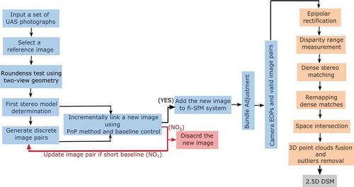
A feature-based incremental SfM (fi-SfM), including first stereo pair selection, image pair combinations and erroneous pair modification, is proposed. The outcomes derived are then used for DSM reconstruction. A previous research proves that ABRISK consumes less computational cost than SIFT (Tsai and Lin 2017) and EABRISK has been developed further (Cheng and Matsuoka 2020) to gain more feature matches, this paper utilizes the recent research and examines its capability for fi-SfM. The second stage presents the procedure to generate dense 3D point clouds from discrete stereo models and automatically combine them as a complete DSM. The workflow designed for 3D reconstruction by using series oblique drone images of unknown camera poses is described in Figure 2. It must be noted that the entire processing is under the coordinate system constructed by fi-SfM. Such a characteristic guarantees that the 3D point clouds produced by discrete stereo models can be merged automatically.

Figure 2. The proposed workflow for feature-based incremental Structure-from-Motion (fi-SfM) and 3D modelling

3.1. Feature-based incremental structure-form-motion

The proposed feature-based incremental structure-from-motion (fi-SfM) is built on SfM, but without the assistance of POS data. Selecting a suitable point of origin and image pair (stereo model) beforehand is important because the short baseline introduces ambiguous 3D points, while long baseline reduces image overlap. In addition, the first pair affects the stability and accuracy of the modelling system. Rather than directly measuring base-high ratio, roundness test exploiting camera EOPs along with the generated sparse 3D points of a stereo model is employed (Beder and Steffen 2006; Hess-Flores, Recker, and Joy 2014). By two-view geometry, the relative positions and rotational angles of two cameras can be estimated using either fundamental or essential matrix (Hartly 1995; Nister 2004); 3D points belonging to a certain image pair can also be computed. To obtain suitable initial estimations, Equation (2)(2) $\lambda \left[\begin{array}{c}u\\ v\\ 1\end{array}\right]=\left[\begin{array}{ccc}f& 0& x_0\\ 0& f& y_0\\ 0& 0& 1\end{array}\right]\left[\begin{array}{cccc}{m}_{11}& m_{12}& m_{13}& t_x\\ m_{21}& m_{22}& m_{23}& t_y\\ m_{31}& m_{32}& m_{33}& t_z\end{array}\right]\left[\begin{array}{c}X\\ Y\\ Z\\ 1\end{array}\right]$(2) along with 5 points algorithm using essential matrix are used. As the roundness test evaluates the quality of 3D points, a larger value indicates that the points derived from the two camera centres are more stable. To efficiently perform this task, a reference image is needed. In this research, the image with the greatest number of detected features is used as the reference, and it is also the point of origin for the modelling system. Afterwards, matching the reference to other images are used to yield a set of roundness values. Determining the most appropriate first image pair is thereby achieved by identifying the largest value with respect to the reference image; as a result, the fi-SfM system is established.

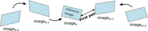
In order to include the remaining images into the modelling system, discrete image pairs are created by determining their spatial linkages. Each pair accounts for the closest spatial linkage between two images. This can be done based on the relative similarity calculated by Jaccard index (Michelini and Mayer 2020). This paper simplifies Jaccard index as the quantity of matches obtained from image matching, and two images of greater relative similarity means that there are more conjugate features. Feature matching is implemented for every image, including the images of the first stereo pair, in order to the pair with the highest correlation. For sequentially ordered dataset showing in Figure 3, there can be more than one pair with the highest correlation (e.g., left and right neighbours) and can result to two stereo models.

Figure 3. Image sequence, similarities and spatial linkages

A further examination to each image pair is required on whether the baselines produce ambiguous 3D points because the baseline of the initial stereo model solved by the essential matrix is normalized to one unit (Nister 2004). Such a procedure can be addressed when adding a new image into the system, where some images have already been spatially linked. Take Figure 3 for example, the EOPs of image${ }_{(k-1)}$ can be estimated through conjugate 2D and 3D points with respect to image${ }_{(k)}$ and the (EPnP) solution (Lepetit, Moreno-Noguer, and Fua 2009), after determining the first pair. As a result, the baseline of the pair of images k-1 and k can be computed using their positional vectors t${ }_{(k-1)}$ and t${ }_{(k)}$. If the length of the baseline is above a threshold, this new image is introduced into the modelling system; meanwhile, new 3D points can be generated by their common features (tie-points). In case the length of the baseline is shorter than the threshold, the proposed method allows that new image to find another source from the images already in the modelling system (NO${ }_1$ in Figure 2). By looking up the discrete image pairs, a new image pair consisting of images k-1 and k+ 1 can be reorganized since images k and k+ 1 are already available, and images k and k-1 are associated. For this improved pair, if the baseline is still shorter than the threshold, image${ }_{(k-1)}$ is considered unsuitable for 3D reconstruction and eliminated (NO${ }_2$) in Figure 2). The threshold is set 0.8 units in this study so as to sidestep ambiguous 3D points caused by short baselines. Otherwise, these ambiguity points might lead to unsuccessful camera EOPs estimations for the succeeding linking of images. This procedure is carried out recursively until all images are processed so that cameras’ EOPs, sparse 3D points and a list of valid image pairs are produced. For image matching, RANSAC is implemented in two-view geometry and PnP problem to eliminate mismatches (outliers), enhancing the stability of the results. This workflow assigns the RANSAC threshold by five pixels to determine correct matches. There are two significant characteristics of this fi-SfM approach: (1) the model scale is arbitrary and unknown invoked by homogeneous coordinate and essential matrix and (2) all cameras’ EOPs attained are relative to the reference image.

Although the modified fi-SfM method can spatially link the images, automatically update image pairs and discard inappropriate data, the influence of error propagation must not be ignored. To further enhance the robustness, bundle adjustment is employed to tweak all EOPs and 3D points by minimizing the intact projection error. Equation (3)(3) $\mathrm{m}\mathrm{i}{\mathrm{n}}_{{\mathbf{a}}_j,p_i}\sum _{i=1}^n\sum _{j=1}^m{g}_{i,j}(\mathbf{Q}({\mathbf{a}}_j,P_i)-p_{i,j}{)}^2$(3) recalls the bundle adjustment calculation, assuming that n-3D-points are seen in m-views. In this equation, p${ }_{i,j}$ accounts for the measurement of i-th 3D point on image j; also, let g denotes binary variables that equal 1 if i-th 3D point is visible in image j, and 0 otherwise. The projection model of Equation (2)(2) $\lambda \left[\begin{array}{c}u\\ v\\ 1\end{array}\right]=\left[\begin{array}{ccc}f& 0& x_0\\ 0& f& y_0\\ 0& 0& 1\end{array}\right]\left[\begin{array}{cccc}{m}_{11}& m_{12}& m_{13}& t_x\\ m_{21}& m_{22}& m_{23}& t_y\\ m_{31}& m_{32}& m_{33}& t_z\end{array}\right]\left[\begin{array}{c}X\\ Y\\ Z\\ 1\end{array}\right]$(2) is marked as Q, predicting the projection of a 3D point (P${ }_i$) onto images where it is visible, and camera orientations are parameterized as a${ }_j$ (= K[M$|$t]${ }_j$). With the predictions as well as their 2D measurements, the Levenberg-Marquardt (LM) and least-squares solution (Kanatani and Sugaya 2011; Verykokou and Ioannidis 2018) aid in optimizing the camera orientations and the sparse 3D points simultaneously. Erroneous 3D points or image pairs, moreover, have an additional opportunity to be detected and disposed of so that the derived spatial information becomes more stable. The aforementioned RANSAC threshold is reused to identify possible erroneous 3D points, which are removed if the gap between the measurement and the projection is greater than five pixels. As a result, bundle adjustment is carried out iteratively until the specific condition is achieved. This paper terminates the processing by either when the total projection error is less than one pixel, or when the error varies marginally compared to the previous operation (0.300 pixels in this research). But because the first stereo model determines the arbitrary scale for the fi-SfM system, the EOPs of the two images are not necessarily modified by bundle adjustment.

(3) $\mathrm{m}\mathrm{i}{\mathrm{n}}_{{\mathbf{a}}_j,p_i}\sum _{i=1}^n\sum _{j=1}^m{g}_{i,j}(\mathbf{Q}({\mathbf{a}}_j,P_i)-p_{i,j}{)}^2$(3)

3.2. Dense point clouds generation

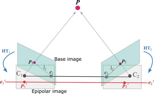
The sparse 3D points derived from fi-SfM are apparently inadequate to present a complete DSM. As SGM-based is still commonly used to obtain substantial matches from an image pair, this paper adopts the simplified SGBM for dense matching because of its efficiency and acceptable results. In order to address this issue, and epipolar stereo model, which reduces the matching complexity from 2D to one-dimensional (1D), is required. Epipolar rectification utilizing POS information was successfully implemented in Cho, Schenk, and Madani (1993) and Tran (2009). An alternative homographic rectification, shown in Figure 4, can also achieve epipolar stereo model by translating and rotating two base images through relative orientation parameters (ROPs) defined in Equation (4)(4) ${\mathbf{M}}_{\mathrm{R}}={\mathbf{M}}_2{\mathbf{M}}_1^{-1}=\left[\begin{array}{ccc}{m}_{11}& m_{12}& m_{13}\\ m_{21}& m_{22}& m_{23}\\ m_{31}& m_{32}& m_{33}\end{array}\right],B=M_1(t_2-t_1)=\left[\begin{array}{c}{b}_x\\ b_y\\ b_z\end{array}\right]$(4) of two cameras (Kim and I.and Kim 2016; Loop and Zhang 1999). In this equation, the relative rotation matrix M${ }_{\mathrm{R}}$ is obtained by two rotation matrices M${ }_1$ and M${ }_2$, and the baseline (B) vector is computed via two positional vectors t${ }_1$ and t${ }_2$, as well as M${ }_1$. Two principles aid in conducting homographic rectification: (1) mapping the two epipoles to a point at infinity (1, 0, 0) along the horizontal axis (e${ }_1$ $\to$ e${ }_1^{\prime }$, e${ }_2$ $\to$ e${ }_2^{\prime }$) and (2) the epipolar lines (l${ }_1$ and l${ }_2$) are distorted being parallel to the baseline (e${ }_1$p${ }_1$ $\to$ e${ }_1^{\prime }$p${ }_1^{\prime }$, e${ }_2$p${ }_2$ $\to$ e${ }_2^{\prime }$p${ }_2^{\prime }$). Three vectors h${ }_1$, h${ }_2$ and h${ }_3$ defined in Equation (5)(5) $h_1=\frac{B}{∥B∥},h_2=\frac{{\left[\begin{array}{ccc}-b_y& b_x& 0\end{array}\right]}^{\mathrm{T}}}{\sqrt{b_x^2+b_y^2}},h_3=h_1\times h_2,{\mathbf{M}}_{\mathrm{r}\mathrm{e}\mathrm{c}\mathrm{t}}=\left[\begin{array}{c}{h}_1^{\mathrm{T}}\\ h_2^{\mathrm{T}}\\ h_3^{\mathrm{T}}\end{array}\right]$(5) comprise the rectification matrices for a stereo pair. The first vector h${ }_1$ coincides with the direction of the baseline, and the two epipoles are also on this vector. The second vector h${ }_2$ is orthogonal to h${ }_1$ with respect to the direction of the optical axis (i.e. z-axis in Figure 1). The unit vector h${ }_3$ accounts for the unambiguity and is determined by the cross product of h${ }_1$ and h${ }_2$. In this equation, $\parallel B\parallel$ accounts for the magnitude of the baseline (B) vector, and T stands for the transpose operator. Consequently, two rectification matrices HT${ }_1$ and HT${ }_2$ in Equation (6)(6) $\begin{array}{c}\mathbf{H}{\mathbf{T}}_1={\mathbf{M}}_{\mathrm{r}\mathrm{e}\mathrm{c}\mathrm{t}}\\ \mathbf{H}{\mathbf{T}}_2={\mathbf{M}}_{\mathrm{R}}^{-1}{\mathbf{M}}_{\mathrm{r}\mathrm{e}\mathrm{c}\mathrm{t}}\end{array}$(6) are computed using the three vectors in Equation (5)(5) $h_1=\frac{B}{∥B∥},h_2=\frac{{\left[\begin{array}{ccc}-b_y& b_x& 0\end{array}\right]}^{\mathrm{T}}}{\sqrt{b_x^2+b_y^2}},h_3=h_1\times h_2,{\mathbf{M}}_{\mathrm{r}\mathrm{e}\mathrm{c}\mathrm{t}}=\left[\begin{array}{c}{h}_1^{\mathrm{T}}\\ h_2^{\mathrm{T}}\\ h_3^{\mathrm{T}}\end{array}\right]$(5) so as to produce epipolar stereo model.

Figure 4. Epipolar rectification by using relative camera poses

(4) ${\mathbf{M}}_{\mathrm{R}}={\mathbf{M}}_2{\mathbf{M}}_1^{-1}=\left[\begin{array}{ccc}{m}_{11}& m_{12}& m_{13}\\ m_{21}& m_{22}& m_{23}\\ m_{31}& m_{32}& m_{33}\end{array}\right],B=M_1(t_2-t_1)=\left[\begin{array}{c}{b}_x\\ b_y\\ b_z\end{array}\right]$(4)

(5) $h_1=\frac{B}{∥B∥},h_2=\frac{{\left[\begin{array}{ccc}-b_y& b_x& 0\end{array}\right]}^{\mathrm{T}}}{\sqrt{b_x^2+b_y^2}},h_3=h_1\times h_2,{\mathbf{M}}_{\mathrm{r}\mathrm{e}\mathrm{c}\mathrm{t}}=\left[\begin{array}{c}{h}_1^{\mathrm{T}}\\ h_2^{\mathrm{T}}\\ h_3^{\mathrm{T}}\end{array}\right]$(5)

(6) $\begin{array}{c}\mathbf{H}{\mathbf{T}}_1={\mathbf{M}}_{\mathrm{r}\mathrm{e}\mathrm{c}\mathrm{t}}\\ \mathbf{H}{\mathbf{T}}_2={\mathbf{M}}_{\mathrm{R}}^{-1}{\mathbf{M}}_{\mathrm{r}\mathrm{e}\mathrm{c}\mathrm{t}}\end{array}$(6)

Disparity range plays an important role when applying SGBM to gauge feature resemblance along the epipolar lines (i.e. x-axes in Figure 5) within a specific interval. As shown in Figure 5(c), it demonstrates that the disparity range constrains the capacity for feature matching by an outset and terminal. An inadequate interval, thus, results in incorrect matches and fails to achieve DSM reconstruction. Moreover, discrete epipolar stereo models have their distinct intervals in terms of disparity range; a uniform interval does not apparently suit each stereo model. Instead of generating an image pyramid to handle this issue (Pierrot-Deseilligny and Paparoditis 2006), this study determines the disparity range automatically and dynamically. By applying EABRISK to an epipolar stereo model, a group of matches serve to measure the disparity range. On the fact that an individual feature pair must locate on the identical epipolar line, the gap between two u coordinates (column domain) thereby draws the disparity range. Among many feature pairs involved, the maximum value of difference defined by Equation (7)(7) $D_{\mathrm{r}\mathrm{a}\mathrm{n}\mathrm{g}\mathrm{e}}=\mathrm{m}\mathrm{a}\mathrm{x}(u_i^{{\mathrm{e}}_2}-u_i^{{\mathrm{e}}_1});i\in \mathrm{l}\mathrm{o}\mathrm{c}\mathrm{a}\mathrm{l}\mathrm{m}\mathrm{a}\mathrm{t}\mathrm{c}\mathrm{h}\mathrm{e}\mathrm{s}\mathrm{i}\mathrm{n}\mathrm{e}\mathrm{p}\mathrm{i}\mathrm{p}\mathrm{o}\mathrm{l}\mathrm{a}\mathrm{r}\mathrm{s}\mathrm{t}\mathrm{e}\mathrm{r}\mathrm{e}\mathrm{o}\mathrm{m}\mathrm{o}\mathrm{d}\mathrm{e}\mathrm{l}$(7) has the most potential disparity range for dense stereo matching. For practical purposes, the disparity interval is confined within (0, D${ }_{\mathrm{r}\mathrm{a}\mathrm{n}\mathrm{g}\mathrm{e}}$). As a consequence, a disparity map is produced to look up conjugate features across two epipolar images. For example, a feature pair can be presented as (u${ }^{\mathrm{e}}$, v${ }^{\mathrm{e}}$) and (u${ }^{\mathrm{e}}$+d, v${ }^{\mathrm{e}}$) in the left and right epipolar views, where d is the disparity value stored in the cell.

Figure 5. Dense feature matching along epipolar lines (a) Semi-global matching by pixel-wise operation; (b)Semi-global matching by template operation; (c) Disparity range for feature resemblances evaluation

(7) $D_{\mathrm{r}\mathrm{a}\mathrm{n}\mathrm{g}\mathrm{e}}=\mathrm{m}\mathrm{a}\mathrm{x}(u_i^{{\mathrm{e}}_2}-u_i^{{\mathrm{e}}_1});i\in \mathrm{l}\mathrm{o}\mathrm{c}\mathrm{a}\mathrm{l}\mathrm{m}\mathrm{a}\mathrm{t}\mathrm{c}\mathrm{h}\mathrm{e}\mathrm{s}\mathrm{i}\mathrm{n}\mathrm{e}\mathrm{p}\mathrm{i}\mathrm{p}\mathrm{o}\mathrm{l}\mathrm{a}\mathrm{r}\mathrm{s}\mathrm{t}\mathrm{e}\mathrm{r}\mathrm{e}\mathrm{o}\mathrm{m}\mathrm{o}\mathrm{d}\mathrm{e}\mathrm{l}$(7)

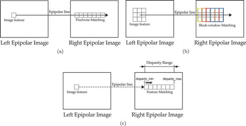
However, it is obvious in Figure 5 that the introduction of SGBM leads to losing the pixel-wise matching capacity, which is an important characteristic of SGM. To compensate for this loss, the weighted least squares (WLS) filter (Strutz 2016) is used during dense matching. Applying this strategy requires two disparity maps derived from forward and backward dense matching as foundations. For each cell in the forward map, its corresponding locations and neighbours (e.g., feature template of size 3 $\times$ 3, 5 $\times$ 5 or 7 $\times$ 7, etc.) in the backward map are extracted for enhancement. With two feature templates, the linear regression is utilized to refine the disparity value of the template centre in the forward map. In addition, cells of empty disparity values can be approximated through bilinear interpolation to gain the most probable estimations. The disparity map can be optimized in order to achieve an effect similar to SGM. In this study, the feature template size of 5 $\times$ 5 is selected to balance the efficiency and moderate outcomes.

To generate 3D point clouds, conventional MVS fuses several depth maps, which is computed through single image 3D projection using disparity map and camera EOPs (Furukawa and Ponce 2010; Li et al. 2010; Rothermel 2017; Shen 2013). Subsequently, spatial constraints are applied to the point clouds in order to verify their correctness. This study conducts space intersection (forward triangulation) using geometric constraints based on cameras’ EOPs and the results of dense stereo matching to procure dense 3D point clouds. The feature pairs extracted from an epipolar stereo model, however, cannot be used directly because the homographic rectification apparently reshapes the image geometry (e.g., principle point x${ }_0$ $\to$ x${ }_0^{\mathrm{e}}$ and y${ }_0$ $\to$ y${ }_0^{\mathrm{e}}$). To use the cameras’ EOPs derived from fi-SfM for space intersection, this study remaps the feature pairs from the epipolar images to their base sources via the rectification matrix, principle point (x${ }_0^{\mathrm{e}}$, y${ }_0^{\mathrm{e}}$) and Equation (8)(8) $\left[\begin{array}{c}{u}^{\prime }\\ v^{\prime }\\ w^{\prime }\end{array}\right]=\mathbf{H}{\mathbf{T}}^{-1}\left[\begin{array}{c}\frac{u^{\mathrm{e}}-x_0^{\mathrm{e}}}{f}\\ \frac{v^{\mathrm{e}}-y_0^{\mathrm{e}}}{f}\\ 1\end{array}\right]$(8) . Therefore, the features’ coordinates in the original images can be recomputed as (u, v) = (u${ }^{\prime }$/w${ }^{\prime }$, v${ }^{\prime }$/w${ }^{\prime }$) for dense 3D point clouds generation. Because the cameras’ EOPs are in an identical coordinate system, the point clouds obtained from each independent stereo model are able to be merged automatically. Lastly, invalid or unlikely 3D points can be removed by using statistical outlier removal (Zhang 2013).

(8) $\left[\begin{array}{c}{u}^{\prime }\\ v^{\prime }\\ w^{\prime }\end{array}\right]=\mathbf{H}{\mathbf{T}}^{-1}\left[\begin{array}{c}\frac{u^{\mathrm{e}}-x_0^{\mathrm{e}}}{f}\\ \frac{v^{\mathrm{e}}-y_0^{\mathrm{e}}}{f}\\ 1\end{array}\right]$(8)

4. Experimental results, analyses and discussions

The Tokyo Institute of Technology – Suzukadai Campus was used as the study area of this research. The series of oblique images was acquired by conventional flight stripes. These images were captured in 2014 with a calibrated Canon EOSM-22 camera model mounted on a simple UAS platform. Table 2 summarizes the camera’s IO parameters, including principle point, focal length, radial distortion parameters A${ }_1$, A${ }_2$, A${ }_3$ and decentring distortion parameters B${ }_1$ and B${ }_1$. There were several limitations in these images. The direct-georeferencing instruments were not included in the platform due to its limiting payload. Although GCPs were also surveyed, they were merely visible due to limitations in the flight plan. In addition, auxiliary information such as overlap rate, spatial resolution (ground sampling distance, GSD) and nadir or near-vertical images were also unavailable. To be able to use these images and achieve 3D reconstruction, a set of eight oblique images shown in Figure 6 were selected from one of the flight strips to test the designed methodology.

Figure 6. Oblique UAS imagery for spatial processing and 3D reconstruction given by the identifications of (a) 1; (b) 2; (c) 3; (d) 4; (e) 5; (f) 6; (g) 7; (h) 8

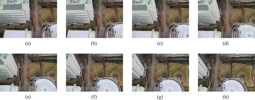
Table 2. Interior orientation parameters of the camera model

Camera model	Canon EOSM-22
Image Size (pixel)	5184^×3456
Principle Point (pixel)	(2641, 1694)
Focal Length (f, pixel)	4991
Lens Distortion	A^1 = 0.020619
	A^2 = −0.176108
	A^3 = 0.826441
	B^1 = −0.000039
	B^2 = −0.000253

4.1. Image pairs selection and camera EOPs recovering

In order to speed up the data processing for fast investigation, the images are downsampled to 1296 $\times$ 864 pixels in the experiment. To correct the principle point offsets and the lens distortions when estimating cameras’ EOPs, the 2D coordinates are normalized by the camera matrix (K). The reference image of this dataset is Figure 6(b) according to the criteria designed, and EOPs of this point of origin are set to zeros. The roundness test between the reference image with respect to the remaining images resulted to most appropriate first stereo model to initiate the modelling environment. In this experiment, an image pair composed of Figure 6(b,c) has the largest roundness value and becomes the first model. In addition, Table 3 records the preliminary image pairs connected by the relative image similarity indices and the optimized results. Two stereo models are reorganized through the proposed tracking strategy due to their invalid baselines in the primitive combinations, and there are no data discarded.

Table 3. Image pairs estimated by relative image similarity and modified pairs and their baselines

Preliminary pair	Updated pair	Baseline	Refined baseline
2 & 3	2 & 3	1.000	1.000
1 & 2	1 & 2	0.915	0.909
3 & 4	3 & 4	1.196	1.046
4 & 5	4 & 5	1.286	1.660
5 & 6	4 & 6	3.055	2.791
6 & 7	5 & 7	2.693	2.536
7 & 8	7 & 8	1.514	0.966

Afterwards, bundle adjustment is carried out to optimize all spatial information derived from fi-SfM. By the cameras’ EOPs, sparse 3D point clouds and stereo combinations are obtained and the total projection error is reduced from 12.540 to 0.380 pixels. Table 3 also lists the baseline of each modified pair before and after bundle adjustment. It is apparent that the lengths of three baselines change significantly pairs 4 & 5, 5 & 6 and 7 & 8 in Table 3), indicating that mismatches remain in these stereo models and are further discovered during the post-refinement. This operation removes erroneous matches inducing invalid 3D points from images, which makes the EOPs more robust. As those modified pairs satisfy the minimal baseline threshold of 0.800 units, they are used to support dense 3D reconstruction without any data discarded.

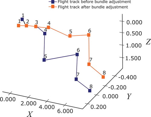
Otherwise, inappropriate image pairs should be omitted. Figure 7 visualizes the flight paths before and after bundle adjustment through the images’ positional information since the primary objective of SfM-driven algorithms is localization. According to this delineation, the shapes of the two flight paths are similar but the positions of later included images are adjusted noticeably. This outcome proves the previous studies of SfM algorithms that error propagation affects the images that are later added into the modelling system, and so does the fi-SfM method. Consequently, their positions are tweaked significantly compared to those ones which are spatially closer to the reference image.

Figure 7. Visualization of flight path recovered by fi-SfM and refined by bundle adjustment

4.2. Digital surface reconstruction

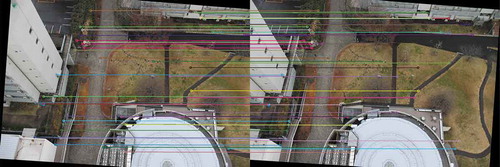
An epipolar stereo model is created for addressing dense stereo matching. As the prerequisite of cameras’ EOPs have been established, epipolar stereo models are then generated by the homographic rectification following the previously defined pairs. Figure 8 demonstrates one of the examples using the last image pair of Figure 6(g–h) (pair 7 & 8 in Table 3) to produce an epipolar stereo model. Although an epipolar image may resemble its original image, common image features within this model are rotated and translated locating on identical scanlines (i.e. x-axis, epipolar line). To verify the epipolar stereo model, the SIFT feature matching is conducted for the two images and randomly extracts 50 samples as shown in Figure 7 to examine their y-parallax (i.e. the difference between image row-counts). The mean square error (MSE) of the y-parallax is equal to 2.320 pixels, showing that each feature pair is spatially aligned on a specific epipolar line. This epipolar stereo model can become the benchmark for dense stereo matching that is capable of evaluating feature similarities along epipolar lines.

Figure 8. An example of epipolar stereo model using image pair (7 & 8) for y-parallax validation and disparity range estimation

By carrying out SGBM with WLS filter using each epipolar stereo model and transferring the disparity map to substantial matches, space intersection using the cameras’ EOPs progressively densifies the sparse 3D point clouds. As shown in Figure 9, the reconstructions derived from the image pairs defined are merged automatically and present a complete DSM. 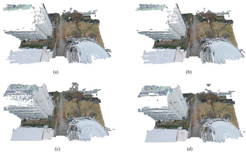The statistical outlier removal setting in this experiment contains two parameters, namely, (1) the quantity of nearest neighbouring points is 20 and (2) the confidential interval is within $\pm$1.5 $\sigma$, where $\sigma$ is the standard deviation of all mean distances computed by every point to its nearest neighbours. Figure 9(a) shows the DSM without WLS filter handling, and Figure 9(b) is the outcome after outlier removal. Similarly, Figure 9(c–d) demonstrate the reconstructions with the improvement of WLS filter. By comparing the DSMs in Figure 9(b) and (d), the quantity of 3D point clouds increases from 3326264 to 4574813, resulting in the accession rate about 37.5%. The consequence shows that the automatic prediction of disparity range for each stereo model is applicable to obtain valid matches for reconstructing a digital surface. In addition, the WLS filter is able to interpolate missing disparity values and generate more point clouds. However, it is evident in the visualization that parts of the scenes are not easily identifiable (Figure 9). A common example is this experiment is the solar panels (refer to the left-top building), which are distinguishable even after the use of a WLS filter. Mixed pixels, such as complicated façades of repeated patterns, uniform texture and occlusions are limitations causing this issue.

Figure 9. Reconstructed DSM through the organized image pairs and the camera EOPs (a), (b) SGBM without using WLS; (c), (d) SGBM with using WLS filter; (b), (d) Reconstructions after outlier removal

The quality assessments are addressed using two indicators, namely, accuracy and completeness. Due to invisible field-measured GCPs in the dataset, this study maps out a group of pseudoground truths as independent check points (ICPs) to examine the completeness of the 3D models. Two solutions are proposed to carry out this issue, First, by manually identifying several points from the images of users’ interests (e.g., a building’s outline) and second, by automatically obtaining them through local keypoints matching (e.g., discrete points). This study opts for SIFT keypoints matching as being opposed to the EABRISK used in the fi-SfM and randomly extracts 50 samples for completeness appraisal. Furthermore, the accuracy assessment is done by measuring six segments in the field and comparing them to the produced DSM.

For completeness evaluation, two 3D models after outlier removal shown in Figure 9(b) and (d) are compared. After acquiring the ICPs, their spatially nearest points in the DSMs are determined by the minimum Euclidean distance. For the given models, therefore, 100 target points are identified. Unsuccessful reconstructions are then determined by identifying models with longer distances between the ICPs and their assigned target points. This study employs statistical detection so as to access the completeness rates. Table 4 shows the results within the confidence interval of 95% (two-tail test). Because the ICPs are selected at random, the values might be merely distinguishable in this evaluation. However, this comparison suggests that dense stereo matching incorporating SGBM with WLS filter still draws its capacity to gain more point clouds to achieve a more complete DSM.

Table 4. Completeness validation of the 3D models

Methodology	Completeness rate	Percentage (%)
SGBM	46/50	92
SGBM with WLS	48/50	96

As demonstrated in Figure 10, there are six segments measured in the field to assess the accuracy of the DSM. The validation data are further classified into two categories, including four segments accounting for horizontal distances (X-Y plane) and two for elevations (Z-direction). In each class, a segment is set as the reference, in which the ratio is equivalent to 1.000, to compute the relative ratio factors of the remainders. These factors are then multiplied by the field-surveyed distance of the reference so that the lengths of the resting segments can be estimated to their true values. Comparisons between the measures and approximations are used for the accuracy assessments of the 3D model. The DSM reconstructed by SGBM with WLS filter is used for the purpose.

Figure 10. Accuracy assessment by field-measured lengths of segments

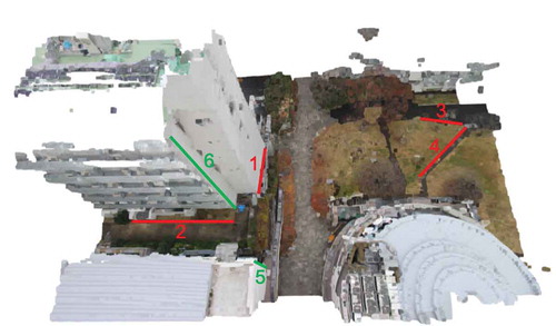
The reference segment in each group is fixed by the shortest distance in the 3D model. Distancing estimations of the resting segments can be computed and compared to their corresponding field-measures, shown in Table 5. After obtaining the differences between approximations and measures, the overall accuracy is 0.235 (m) in this experimental result. The resolving power, moreover, can be roughly computed by the MSE of y-parallax (2.320 pixels), resulting in the GSD of about 10.129 (cm) in the downsampled imagery data. The probable spatial resolution of the raw images can be approximated by 2.532 (cm). Therefore, the general accuracy of the DSM produced by UAS images is expected to be better than the consequence reported in this paper because the spatial resolution is usually high because of its low flying altitude. The possible reasons for the low accuracy may be the downsampled image dataset for faster processing, trapezoidal object caused by oblique image’s capturing and varying spatial resolution of each pixel within an oblique image. However, the spatial information extracted through the proposed workflow can adequately generate the DSM from a series of oblique UAS imagery when the prior camera information is not available.

Table 5. Accuracy assessment of the 3D reconstruction

Segment ID	Model distance	Ratio	Measured distance (m)	Estimated distance (m)
Horizontal segment
1	2.2047	1.000	10.050	10.050
2	4.2599	1.932	19.050	19.418
3	2.3965	1.087	10.847	11.106
4	4.3421	1.969	20.705	19.959
Vertical segment
5	3.6745	1.000	8.894	8.894
6	9.9657	2.712	24.232	24.122

5. Conclusions

This paper explores the workflow of harnessing sequential oblique UAS images for 3D reconstruction when the POS is unavailable or little auxiliary information is known. To spatially associate a succession of these images, phases of two-view geometry, PnP algorithm and BA are assembled to carry out the incremental SfM that relative camera poses and sparse 3D points can be established. Of them, two-view geometry initializes the 3D modelling environment and PnP algorithm aids to spatially associate new images added into the system. The last step utilizes BA to minimize the projection error by tweaking the estimated camera poses as well as the sparse 3D point clouds such that the camera poses become optimal. The assemble approach is able to unify the relative camera poses and sparse 3D point clouds in the coordinate system of a single but arbitrary scale factor. To complete the digital surface reconstruction, the camera poses are further applied to generate dense 3D point clouds by epipolar stereomodel rectification so that SGM/SGBM can address dense feature matching. In this stem, the local feature matching plays a versatile role not only in estimating relative camera poses but also serving feasible disparity range approximation for SGM/SGBM. For dense 3D modelling, this study remaps the feature correspondences from epipolar stereo images to their base images that point clouds generated by independent stereomodels can merge automatically because all spatial information is confined in the coordinate system built by SfM.

The experimental outcomes report that incremental SfM can achieve robust camera poses and point out unsuitable images for DSM reconstruction. This paper particularly neutralizes stereomodels of short baselines because they might cause noisy 3D point clouds, which are inappropriate to put forward the authentic land surface. To verify the quality of 3D reconstruction, this paper utilizes sparse pseudo-ICPs to evaluate the completeness and field-measured segments to access the accuracy. The completeness rate appraised by 50 random ICPs and two-tail test interprets that most land surface can be successfully reconstructed by more than 90%, except for scenes containing mixed pixels, which are dismantled in the 3D model. The accuracy validation also interprets the DSM reconstructed is reliable for further applications, such as instant hazard investigation and rapid decision-support service. For future works, more images will be included because SfM is capable of putting thousands of images together. Furthermore, this work might be improved by incorporating with adequate and well-distributed GCPs in the scenes and nadir images such that geometry constraints in the real-world domain yield the reconstruction to meet the demands for diversified applications.

Acknowledgements

The UAS images were provided by PASCO CORPORATION, Japan.

Disclosure statement

The authors declare no conflict of interest.

Data availability

Due to the campus security concern, participants of this study did not agree for their data to be shared publicly, so supporting data is not available.

Additional information

Funding

A part of this study was supported by JSPS KAKENHI (19H02408).Japan Society for the Promotion of Science

References

- Aicardi, I., F. Chiabrando, N. Grasso, A. M. Lingua, F. Noardo, and A. Spanó. 2016. “Uav Photogrammetry with Oblique Images: First Analysis on Data Acquisition and Processing.” ISPRS Ann. Photogramm. Remote Sens. Spatial Inf. Sci XLI-B1: 835–842.
- Al-Rawabdeh, A., F. He, A. Moussa, N. El-Sheimy, and A. Habib. 2016. “Using an Unmanned Aerial Vehicle-based Digital Imaging System to Derive a 3d Point Cloud for Landslide Scarp Recognition.” Remote Sensing 8: 95.
- Bay, H., T. Tuytelaars, and V. Gool. 2006. “Surf: Speeded up Robust Features.” Computer Vision – ECCV 2006 3951: 404–417.
- Beder, C., and R. Steffen. 2006. “Determining an Initial Image Pair for Fixing the Scale of a 3d Reconstruction from an Image Sequence.” Pattern Recognition 4174: 657–666.
- Birchfield, S., and C. Tomasi. 1998. “A Pixel Dissimilarity Measure that Is Insensitive to Image Sampling.” IEEE Transactions on Pattern Analysis and Machine Intelligence 20 (4): 401–406.
- Börlin, N., A. Murtiyoso, P. Grussenmeyer, F. Menna, and E. Nocerino. 2019. “Flexible Photogrammetric Computations Using Modular Bundle Adjustment: The Chain Rule and the Collinearity Equations.” PE&RS 85 (5): 361–368 (8).
- Bradski, G. 2000. “The Opencv Library”. Dr Dobb’s J. Software Tools, 25, 120-125
- Carrivick, J., M. Smith, and D. Quicey. 2016. Structure from Motion in Geosciences. Chichester, UK: Wiley.
- Cheng, M., and M. Matsuoka. 2020. “An Enhanced Image Matching Strategy Using Binary-stream Feature Descriptors.” IEEE Geoscience and Remote Sensing Letters 17 (7): 1253–1257.
- Cho, W., T. Schenk, and M. Madani. 1993. “Resampling Digital Imagery to Epipolar Geometry.” The International Archives of the Photogrammetry, Remote Sensing 29: 404–408.
- Colomina, I., and P. Molina. 2014. “Unmanned Aerial Systems for Photogrammetry and Remote Sensing: A Review.” ISPRS Journal of Photogrammetry and Remote Sensing 92: 79–97.
- Elnima, E. 2015. “A Solution for Exterior and Relative Orientation in Photogrammetry, A Genetic Evolution Approach.” Journal of King Saud University - Engineering Sciences 27 (1): 108–113.
- Fischler, M. 1980. “Random Sample Consensus: A Paradigm for Model Fitting with Applications to Image Analysis and Automated Cartography.” Communications of the ACM 1087: 381–395.
- Fraser, C. 2018. Sfm and Photogrammetry: What’s in a Name? In Proceedings of the ISPRS Technical Comission II: Symposium 2018 “Towards Photogrammetry 2020”, Riva del Garda, Italy, 3–7 June.Riva del Garda, Italy.
- Furukawa, Y., and J. Ponce. 2010. “Accurate, Dense, and Robust Multiview Stereopsis.” IEEE Transactions on Pattern Analysis and Machine Intelligence 32 (8): 1362–1376.
- Gabrlik, P. 2015. “The Use of Direct Georeferencing in Aerial Photogrammetry with Micro Uav.” IFAC-PapersOnLine 48 (4): 380–385. 13th IFAC and IEEE Conference on Programmable Devices and Embedded Systems.
- Granshaw, S. 2018. “Structure from Motion: Origins and Originality.” The Photogrammetry Record 33: 6–10.
- Granshaw, S., and C. Fraser. 2015. “Computer Vision and Photogrammetry: Interaction or Introspection?” The Photogrammetric Record 30 (149): 3–7.
- Grün, A. 1982. “The Accuracy Potential of the Modern Bundle Block Adjustment in Aerial Photogrammetry.” PE&RS 48 (1): 45–54.
- Habib, A. F., and A. M. Pullivelli 2005. Camera Stability Analysis and Geo-referencing. Proceedings. 2005 IEEE International Geoscience and Remote Sensing Symposium, 2005. IGARSS ’05., 1169–1172.Seoul, South Korea.
- Hartley, R., and J. Mundy 1993. Relationship between Photogrammmetry and Computer Vision. Proc. SPIE 1944, Integrating Photogrammetric Techniques with Scene Analysis and Machine Vision, 1944.Orlando, FL, United State.
- Hartly, R. 1995. In Defence of the 8-point Algorithm. Proc. 5th International Conference on Computer Vision, 1064–1070.Cambridge, Massachusetts: Massachusetts Institute of Technology.
- Hartly, R., and A. Zisserman. 2004. Multiple View Geometry in Computer Vision -. 2nd ed. Cambridge University Press.
- Harwin, S., and A. Lucieer. 2012. “Assessing the Accuracy of Georeferenced Point Clouds Produced via Multi-view Stereopsis from Unmanned Aerial Vehicle (Uav) Imagery.” Remote Sensing 4 (6): 1573–1599.
- He, F., and A. Habib. 2014. “Linear Approach for Initial Recovery of the Exterior Orientation Parameters of Randomly Captured Images by Low-cost Mobile Mapping Systems.” The International Archives of the Photogrammetry, Remote Sensing and Spatial Information Sciences XL-1: 149–154.
- Hess-Flores, M., S. Recker, and K. I. Joy 2014. Uncertainty, Baseline, and Noise Analysis for L1 Error-based Multi-view Triangulation. 2014 22nd International Conference on Pattern Recognition, 4074–4079. Stockholm, Sweden.
- Hirschmuller, H. 2005. Accurate and Efficient Stereo Processing by Semi-global Matching and Mutual Information. 2005 IEEE Computer Society Conference on Computer Vision and Pattern Recognition (CVPR’05), 2, 807–814. San Diego, California.
- Hirschmuller, H. 2007. “Stereo Processing by Semiglobal Matching and Mutual Information.” IEEE Transactions on Pattern Analysis and Machine Intelligence 30 (2): 328–341.
- Hirschmuller, H. 2011. “Semi-global Matching - Motivation, Developments and Applications.” Photogrammetric Week 11: 173–184.
- Huang, P., K. Matzen, J. Kopf, N. Ahuja, and J. Huang 2018. Deepmvs: Learning Multiview Stereopsis. 2018 IEEE/CVF Conference on Computer Vision and Pattern Recognition (CVPR’18), 2821–2830. Salt Lake City, UT, USA.
- Jiang, S., and W. Jiang. 2018. “Efficient Sfm for Oblique Uav Images: From Match Pair Selection to Geometrical Verification.” Remote Sensing 8: 10.
- Jiang, S., and W. Jiang. 2020. “Efficient Match Pair Selection for Oblique Uav Images Based on Adaptive Vocabulary Tree.” ISPRS Journal of Photogrammetry and Remote Sensing 161: 61–75.
- Kanatani, K., and Y. Sugaya. 2011. Bundle Adjustment for 3-d Reconstruction: Implementation and Evaluation, 45. Okayama University.
- Kim, T., and J. I.and Kim. 2016. “Comparison of Computer Vision and Photogrammetric Approaches for Epipolar Resampling of Image Sequence.” Sensors 16 (3): 412.
- Kyung, M.-H., M.-S. Kim, and S. Hong. 1996. “A New Approach to Through-the-lens Camera Control.” Graphical Models and Image Processing 58 (3): 262–285.
- Lepetit, V., F. Moreno-Noguer, and P. Fua. 2009. “Epnp: An Accurate O(n) Solution to the Pnp Problem.” International Journal of Computer Vision 81: 155.
- Leutenegger, S., and M. Chli2011. Brisk: Binary Robust Invariant Scalable Keypoints. 2011 International Conference on Computer Vision (ICCV’11), 2548–2555. Barcelona, Spain.
- Li, J., E. Li, Y. Chen, L. Xu, and Y. Zhang 2010. Bundled Depth-map Merging for Multiview Stereo. 2010 IEEE Computer Society Conference on Computer Vision and Pattern Recognition (CVPR’10), 2769–2776. San Francisco, CA, USA.
- Liu, J., L. Zhang, Z. Wang, and R. Wang. 2020. “Dense Stereo Matching Strategy for Oblique Images that Considers the Plane Directions in Urban Areas.” IEEE Transactions on Geoscience and Remote Sensing 58 (7): 5109–5116.
- Loop, C., and Z. Zhang 1999. Computing Rectifying Homographies for Stereo Vision. Proceedings. 1999 IEEE Computer Society Conference on Computer Vision and Pattern Recognition (Cat. No PR00149), 1, 125–131. Fort Collins, CO, USA.
- Lowe, D. G. 2004. “Distinctive Image Features from Scale-invariant Keypoints.” International Journal of Computer Vision 60 (2): 91–110.
- Lu, X. 2018. “A Review of Solutions for Perspective-n-point Problem in Camera Pose Estimation.” Journal of Physics 1087: 052009.
- Luhmann, T., C. Fraser, and H. Maas. 2016. “Sensor Modelling and Camera Calibration for Close-range Photogrammetry.” ISPRS Journal of Photogrammetry and Remote Sensing 115: 37–46.
- Luhmann, T., R. Stuart, K. Stephen, and B. Jan. 2013. Close-range Photogrammetry and 3d Imaging -. 3rd ed. De Gruyter. Berlin, Germany.
- Mahler, C. F., E. Varanda, and L. C. D. de Oliveira. 2012. “Analytical Model of Landslide Risk Using Gis.” Open Journal of Geology 2: 3.
- Mian, O., J. Lutes, G. Lipa, J. J. Hutton, E. Gavelle, and S. Borghini. 2015. “Direct Georeferencing on Small Unmanned Aerial Platforms for Improved Reliability and Accuracy of Mapping without the Need for Ground Control Points.” The International Archives of the Photogrammetry, Remote Sensing and Spatial Information Sciences XL-1/W4: 397–402. XL-1/W4.
- Michelini, M., and H. Mayer. 2020. “Structure from Motion for Complex Image Sets.” ISPRS Journal of Photogrammetry and Remote Sensing 166: 140–152.
- Nex, F., E. Rupnik, and F. Remondino. 2013. “Building Footprints Extraction from Oblique Imagery.” ISPRS Ann. Photogramm. Remote Sens. Spatial Inf. Sci: 61–66. II-3/W3.
- Nister, D. 2004. “An Efficient Solution to the Five-point Relative Pose Problem.” IEEE Transactions on Pattern Analysis and Machine Intelligence 26 (6): 756–770.
- Pan, Y., Y. Dong, D. Wang, A. Chen, and Z. Ye. 2019. “Three-dimensional Reconstruction of Structural Surface Model of Heritage Bridges Using Uav-based Photogrammetric Point Clouds.” Remote Sensing 11: 1024.
- Pierrot-Deseilligny, M., and N. Paparoditis. 2006.“A Multiresolution and Optimization-based Image Matching Approach: An Application to Surface Reconstruction from Spot5-hrs Stereo Imagery.” ISPRS Ann. Photogramm. Remote Sens. Spatial Inf. Sci. 36: 1/W41.
- Qin, R. 2014. “An Object-based Hierarchical Method for Change Detection Using Unmanned Aerial Vehicle Images.” Remote Sensing 6: 7911–7932.
- Rothermel, M. 2017. Development of a sgm-based multi-view reconstruction framework for aerial imagery ( Unpublished doctoral dissertation). University of Stuttgart.
- Rothermel, M., K. Gong, D. Fritsch, K. Schindler, and N. Haala. 2020. “Photometric Multiview Mesh Refinement for High-resolution Satellite Images.” ISPRS Journal of Photogrammetry and Remote Sensing 166: 52–62.
- Rublee, E., V. Rabaud, K. Konolige, and G. Bradski 2011. Orb: An Efficient Alternative to Sift or Surf. 2011 International Conference on Computer Vision (ICCV’11), 2564–2571. Barcelona, Spain.
- Rupnik, E., F. Nex, and F. Remondino 2014. “Oblique Multi-camera Systems – Orientation and Dense Matching Issues”. Int. Arch. Photogramm. Remote Sens. Spatial Inf. Sci., XL-3/W1, 107–114.
- Seitz, S., B. Curless, J. Diebel, D. Scharstein, and R. Szeliski 2006. A Comparison and Evaluation of Multi-view Stereo Reconstruction Algorithms. 2006 IEEE Computer Society Conference on Computer Vision and Pattern Recognition (CVPR’06), 1, 519–528.New York, NY.
- Shen, S. 2013. “Accurate Multiple View 3d Reconstruction Using Patch-based Stereo for Largescale Scenes.” IEEE Transactions on Image Processing 22 (5): 1901–1914.
- Siebert, S., and J. Teizer. 2014. “Mobile 3d Mapping for Surveying Earthwork Projects Using an Unmanned Aerial Vehicle (Uav) System.” Automation in Construction 41: 1–14.
- Strutz, T. 2016. Data Fitting and Uncertainty - a Practical Introduction to Weighted Least Squares and beyond -. 2nd ed. Germany: Vieweg+Teubner, Wiesbaden.
- Szeliski, R. 2010. Computer Vision: Algorithms and Applications. New York, USA: Springer.
- Tanathong, S., and I. Lee. 2010. “Speeding up the Klt Tracker for Real-time Image Georeferencing Using Gps/ins Data.” Korean Journal of Remote Sensing 26: 629–644.
- Toschi, I., E. Nocerino, F. Remondino, A. Revolti, G. Soria, and S. Piffer. 2017. “Geospatial Data Processing for 3d City Model Generation, Management and Visualization.” The International Archives of the Photogrammetry, Remote Sensing and Spatial Information Sciences XLII-1: 527–534..
- Tran, T. 2009. “Epipolar Resampling of Stereo Image Base on Airbase in the Digital Photogrammetry”. 7th FIG Regional Conference. Hanoi, Vietnam.
- Triggs, B., P. McLauchlan, R. Hartley, and A. Fitzgibbon 2000. “Bundle Adjustment – A Modern Synthesis”. Vision algorithms: theory and practice, lncs, 298–375.
- Tsai, C., and Y. Lin. 2017. “An Accelerated Image Matching Technique for Uav Orthoimage Registration.” ISPRS Journal of Photogrammetry and Remote Sensing 128: 130–145.
- Tumurbaatar, T., and T. Kim 2018. Comparision of Computer Vision and Photogrammetric Approaches for Motion Estimation of Object in an Image Sequence. 2018 IEEE 3rd International Conference on Image, Vision and Computing (ICIVC), 581–585. Chongqing, China.
- Verykokou, S., and C. Ioannidis 2018. “A Photogrammetry-based Structure from Motion Algorithm Using Robust Iterative Bundle Adjustment Techniques”. ISPRS Ann. Photogramm. Remote Sens. Spatial Inf. Sci., IV-4/W6, 73–80.
- Westoby, M., J. Brasington, N. Glassera, M. Hambrey, and J. Reynolds. 2012. “Structure- From-motion’ Photogrammetry: A Low-cost, Effective Tool for Geoscience Applications.” Geomorphology 179: 300–314.
- Wojciechowska, G., and J. Łuczak 2018. “Use of Close-range Photogrammetry and Uav in Documentation of Architecture Monuments”. E3S Web Conf. XVIII Conference of PhD Students and Young Scientists “Interdisciplinary Topics in Mining and Geology, 71.
- Wolf, P., B. Dewitt, and B. Wilkinson. 2014. Elements of Photogrammetry with Applications in Gis -. 4th ed. New York, NY, USA: McGraw-Hill Science.
- Zhang, J. 2013. “Dense Point Could Extraction from Oblique Imagery”. (Unpublished master’s thesis). Rochester Institute of Technology.
- Zhang, J., M. Boutin, and D. Aliaga 2006. “Robust Bundle Adjustment for Structure from Motion”. 2006 International Conference on Image Processing, 2185–2188. Atlanta, GA, USA.