Remote sensing versus the area sampling frame method in paddy rice acreage estimation in Indramayu regency, West Java province, Indonesia

ABSTRACT

With a population of 267 million, Indonesia faces the significant challenge of inaccurate rice production data leading to a flawed national rice import policy and supply problems. Its 2018 rice production and harvest area data were generated through the Area Sampling Frame (ASF) method which incurred high labour and financial costs as well as failing to optimize accuracy; hence, an alternative method needs exploration. This study compares ASF and remote sensing Synthetic Aperture Radar (SAR) methods to calculate rice growth stages (RGS) using Indramayu Regency, the highest rice producer in West Java Province, as the study area. The SAR-based method used time-series of Vertical Horizontal (VH) polarization of Sentinel-1A data that employed a combination of k-means clustering, hierarchical cluster analysis (HCA), a visual interpretation and support vector machine (SVM) classifier. Both SAR and ASF methods can generate results on a monthly basis, although remote sensing satellite time revisits can be shortened (every 12 days). Whilst the ASF, a basic technique for collecting agricultural statistics, was easy to implement in large-scale areas its accuracy depended on the quantity and representativeness of the samples. This study applied the ASF by simulating a sample size of 1.7%, 3.3% and 5% of a rice field area with unmanned aerial vehicles (UAVs) data as a reference. Whilst remote sensing SAR methods involve complex data processing the image classification process can be conducted automatically and cost-effectively (data and its software are free of charge). Moreover, it yields not only statistical data on RGS but also determines the spatial planting patterns and the RGS distribution at 10 m pixel resolution. This method showed more accurate results with overall accuracy of image classification of 81.89% and a kappa coefficient (κ) of 0.73. The comparative result was relatively small, i.e., 4,094.89 ha more than the ASF results (3.5% difference), since this study covered a limited research area. Nonetheless, with evidence of more accurate results remote sensing holds the potential for replication across the country’s 416 regencies, so enabling government to develop more appropriate policies that minimize the risks of either a surplus or shortage in the nation’s most important food supply.

1. Introduction

Rice is the main food staple for more than three and a half billion of the world’s population with consumption per capita of 53.7–57.9 kg in 2017–2018 (FAO 2018). In 2018 the global rice harvested area reached 163.47 million ha, or 11.5% of the total agricultural area (USDA 2019). In the same year the world’s rice production reached 769.9 million tonnes with 88% produced in South, East, and Southeast Asia (FAO (Food and Agriculture Organization) 2018). Problems arise when populations increase and rice consumption per capita (demand) exceeds production (supply), the latter relating immediately to the issue of land availability and its productive capacity. This issue is exacerbated by the negative impact of climate change, especially the increasing temperature with the potential to shorten the duration of plant growth and thereby decrease yields (Zhang et al. 2017). These factors challenge the ability of a country to maintain sufficient food supplies (Kuenzer and Knauer 2013; Xu et al. 2019).

Indonesia is the world’s third-largest rice producer after China and India, with 83.04 million tonnes produced in 2018 (FAO 2020). The current government released nine priority programmes called ‘Nawa Cita’ (Kominfo 2015), initiated to ensure that Indonesia retains its political sovereignty, is independent economically and remains strong culturally (Neilson and Wright 2017). Achieving food sovereignty through increased rice production is central to this policy and challenged by the inaccuracy of rice data, and specifically how a rice harvest area is measured and calculated (BPS 2018a). These two processes are mainly carried out by the simple estimation of an ‘officer’s eye view’ and thus difficult to achieve a high level of accuracy (Mubekti and Sumargana 2016). Invalid data results in inappropriate policies, including incorrect rice imports which is often cited as a major cause of national supply problems (Gaffar 2013; Aryani 2018). In September 2018 the head of the state-owned logistics company (‘Bulog’) publicly stated that their data on rice reserves differed from that held by the Ministry of Trade leading to controversy on rice import policy.

In 2017 five state institutions, led by Statistics Indonesia (Badan Pusat Statistik/BPS) and the Agency for the Assessment and Application of Technology (Badan Pengkajian dan Penerapan Teknologi/BPPT), collaborated to improve the country’s rice data by applying the Area Sampling Frame (ASF) method (BPS, 2018a). The ASF method, developed in the early 1990s by the BPPT with the European Union (Mubekti and Hendrarto 2010), is implemented through the Government’s guided steps for ASF development. The key steps include: vector map collection of rice fields within sub-regency administrative boundaries; stratification of irrigation-based or rainfed rice fields; construction and overlaying large and sub-grids; attribution of each grid with an id and name or sub-regency, regency, and province as well as their location, stratification category, etc.; field observation of rice growth stages and data reporting to the servers. However, until 2017 ASF implementation was still in the pilot project stage in several regencies in Java Island. Moreover, previously the reporting system from field officers was performed in paper form and then transformed into a short message service, a process that undermined its progress (Munandar 2014). The method has been enhanced through the use of the internet, the Global Positioning System (GPS) and the Geographic Information System (GIS), all of which are available from Android smartphones. Together these increase the ASF’s economic and technological viability, and since 2018 are now fully operational with high accuracy in measuring and calculating the rice harvest area (Agustan et al. 2018).

Another means for producing rice data is through the use of phenology-based remote sensing with the ability to map and monitor rice fields on a wide scale quickly and accurately. This method has been applied with accuracy of 82% to 95% in various countries including in the United States (Sousa and Small 2019), Turkey (Rufin et al. 2019), France (Bazzi et al. 2019), China (Mansaray et al. 2019), India, Vietnam, Cambodia, Thailand, the Philippines and Indonesia (Nelson et al. 2014). In tropical island countries such as Indonesia, with relatively high air humidity (an average of more than 90%), high rainfall, high temperatures and heavy cloud, medium and long wave remote sensing SAR methods are believed to be more effective than ground-based approaches (Mosleh, Hassan, and Chowdhury 2015; Mansaray et al. 2019).

The advantages and disadvantages of using remote sensing in rice fields mapping were highlighted by Mosleh, Hassan, and Chowdhury (2015), summarized as follows. Firstly, if the sensors rely on the use of solar energy, such as ‘Landsat 8ʹ, it is challenging to secure historical data that is completely cloud-free throughout the entire stage of rice growth. Nonetheless, Landsat-8 (comprising 11 multispectral bands, spatial resolution of 15–100 m and time revisit of 16 days) is considered to be more intuitive, provides better spectral resolution and does not require as much pre-processing compared to SAR imagery. Secondly, if a ‘SAR sensor’ is used the biggest challenge relates to the availability, cost and classification method of data. SAR sensor such as Radarsat-2 C-band, which acquires data every 24 days with a swath width of 100 km (standard mode, spatial resolution of 12.5 m × 12.5 m in range and azimuth), faces application challenges such as lower temporal resolution, low data availability and high cost of data acquisition. Moreover, complex data pre-processing and classification methods add to the challenges.

Responding to these challenges the European Space Agency (ESA) launched SAR Sentinel-1 (A and B) satellites in 2014 and 2016, providing free data together with its data processing software ‘Sentinel-1 toolbox’. From the same relative orbit, these C-band-based SAR satellites are able to cover most regions of the world with an interferometric wide (IW) swath mode (swath width of 250 km; spatial resolution of 5 m × 20 m in range and azimuth) (Neelmeijer et al. 2018). The time revisit of the Sentinel-1A satellite for IW swath mode is 4 days for the European region and at least every 12 days for other regions (Nguyen, Gruber, and Wagner 2016). Coupled with Sentinel-1B, data availability for the European region is thus doubled although Sentinel 1-B is not always available to other regions. Whilst a higher temporal resolution of satellite imagery is favourable for capturing temporal responses of rice phenology, several studies that solely used Sentinel-1A showed sufficient results with an overall accuracy higher than 85% (Chen et al. 2016; Nguyen, Gruber, and Wagner 2016; Lasko et al. 2018; Son et al. 2018). In short, SAR Sentinel-1A data, whose advantages include its high spatial resolution and shorter revisit period, has significant potential for utilization in Indonesia to map and monitor rice harvest area as it addresses geographical, technical and financial challenges. This present study compares the effectiveness of this ‘remote sensing SAR’ method with the ‘ASF’ method.

In so doing this study adopted methods proposed by Rudiyanto et al. (2019) in utilizing time-series Sentinel-1A data in generating rice distribution area, cropping patterns and the spatio-temporal distribution of rice growth stages (RGS) by applying k-means clustering, hierarchical cluster analysis (HCA) and Support Vector Machine (SVM) algorithms sequentially. The advantage of using a combination of the k-means classifier and HCA is that the resulting cluster can show the gradient of the planting schedule (Rudiyanto et al. 2019). Moreover, the SVM, one of two most commonly used machine learning algorithms in remote sensing paddy rice mapping, holds several advantages including its ability to: (i) generalize high-dimensional data from a relatively small number of samples (Mountrakis, Im, and Ogole 2011), (ii) solve a nonlinearly separable data set using kernel functions, and (iii) model nonlinear decision boundaries resulting from using nonlinear kernels (Yang and Cervone 2019). When compared with the use of other methods, such as random forests (RF), the SVM is fairly robust against overfitting especially in high-dimensional data. The former tends to overfit (Kho 2019), a characteristic that also applies to the artificial neural network (ANN) method (Ren 2012). Furthermore, and in contrast to ANN, SVM is resilient to becoming trapped in local minima which enables the classifier to identify the optimal solution consistently (Mountrakis, Im, and Ogole 2011) with less complexity in computational processing (Thanh Noi and Kappas 2018). With the above-mentioned advantages, the use of unsupervised and classifiers for mapping rice areas at different stages warrants justification.

A large body of literature has discussed various methods for mapping and measuring land and rice harvesting area but none has compared the level of accuracy between the ‘remote sensing SAR Sentinel-1ʹ method and the ‘ASF ground-based survey’. For example, several studies have examined the use of the ASF method to obtain general land use and agricultural statistical data (Gonzalez-Alonso et al. 1997; Boryan and Yang 2017; Dong et al. 2017; Sun et al. 2018) but not specifically to observing the rice-growth stage on a monthly basis. This study fills this research gap by determining the difference in the accuracy of the two arguably most appropriate methods for use in Indonesia (i.e., the ASF method and Remote sensing SAR Sentinel-1A). The fastest and most reliable of these two can then be selected and rendered operational to generate the most accurate data on the rice harvest area. This is crucial for the government’s policy planners and decision-makers when formulating appropriate policies concerning the risks of a surplus or shortage in the nation’s food supply. Using the Indramayu Regency as a study area this research aims to: (1) calculate rice growth stages area using both the ASF and the remote sensing SAR Sentinel-1 methods; and (2) compare the accuracy and effectiveness of the estimated rice growth stages area using these two methods. In so doing this study contributes not only to the debate on the accuracy of these two methods but also to the literature on food security in Southeast Asia and Indonesia in particular.

2. Study area

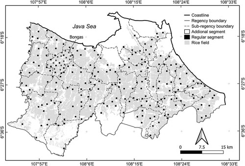
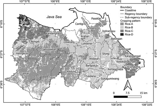
The Indramayu Regency in West Java Province (Figure 1) and Bongas sub-regency were chosen as the study area for several key reasons.

Figure 1. Study area: Indramayu Regency

Up to 58.48% of Indramayu’s total land area (122,000 ha) consists of paddy fields, making it the highest producer of rice in the province with the production of 1,391,928 tonnes of milled dry rice in 2018 (BPS 2018c). The annual planting rice calendar in Indramayu is mainly divided into two seasons. Planting Season I takes place in the rainy season from October to March, while Planting Season II is conducted throughout the dry season from April to September (Kementan 2019) (See Figure 2).

Figure 2. Cropping calendars of rice crops in Indramayu regency in 2018/2019 modified from.Kementan (2019)

The majority of rice fields, i.e., 95,689 ha (BPS 2018b), are irrigated by water sourced from two of the nation’s largest reservoirs. They are the Jatiluhur Reservoir located in Purwakarta Regency and the Jatigede reservoir in Sumedang Regency (Rahman 2019). With sufficient water supply from these reservoirs Indramayu’s rice fields are generally harvested twice a year. To maximize land use rice fields are also planted with cash crops such as soybeans, watermelons and nuts between the rainy and dry seasons (Rudiyanto et al. 2019). The dominant rice variety planted throughout the regency is the Ciherang (80%) with a planting period of 116–125 days (Sitorus 2012). Other varieties include the Mekongga (120 days) and Inpari, Sintanur and the Cilamaya Muncul (126–130 days) (Sitorus 2012; Kementan 2019).

3. Material

This study utilizes three main sets of data: ASF segments, unmanned aerial vehicles (UAVs) and Sentinel-1A. The ASF data were obtained from Statistics Indonesia (Badan Pusat Statistik/BPS) where surveys would typically be conducted simultaneously throughout the country during the last seven days of each month. In this study the data was the coordinates of the GPS points of 216 ‘ASF regular segments’ from October 2018 to September 2019 that cover Indramayu and its respective RGS. ‘Regular’ means that the total number of segments and their positions for conducting an ASF survey remain the same every month. The 216 ASF segments amount to 1.67% of rice fields in the regency. Since this study also focused on the Bongas sub-regency the eight regular segments (1.57%) in the area were combined with an additional 16 new segments to fulfil 5% sample segments of rice field in Bongas. Surveys for these additional segments were conducted coincidentally with the ASF surveys for the regular segments on 24–27 June 2019, and thereby a total of 24 ASF segments were available for Bongas in June 2019. The distribution of all ASF segments, both regular and additional, is depicted in Figure 3.

Figure 3. Distribution of 216 regular and 16 additional ASF segments in Indramayu

By employing ASF methods the aforementioned ASF regular data were used to calculate RGS area throughout Indramayu. In this study, 70% of the data were randomly used as the ground truth data to assist in classifying SAR Sentinel-1A image, while the remainder was used for accuracy assessment. The combination of 8 to 24 sample segments in the Bongas sub-regency was used to calculate its RGS area. In order to further enhance the accuracy assessment UAVs data that covered the Bongas sub-regency area was used as reference data. The UAVs acquisition data covered around 4,900 ha and was generated by the Agency for the Assessment and Application of Technology (BPPT) and BPS on 19–21 June 2019. Meanwhile, the 10 cm ground spatial distance UAVs ortho-mosaicked image (assisted with GPS points of ground truth data) was interpreted visually for producing detailed RGS map with a scale of 1:200. Google Earth images with a resolution of 15–30 cm (Google 2019) were also used as reference data to differentiate rice and non-rice field areas.

This study also used 29 time-series of descending mode SAR Sentinel-1A data from October 2018 to September 2019 (from https://scihub.copernicus.eu). Only Sentinel-1A satellite imagery was utilized since Sentinel-1B was not available in the study area. Sentinel-1 satellite carries a SAR C-band sensor that produces dual polarimetry data in the form of vertical wave reception/vertical transmission and horizontal wave (VV/VH) with a spatial resolution of 5 m × 20 m. The product data used were Interferometric Wide Swath Mode (IW) Level-1 ground-range detected (GRD).

VH polarization data were chosen explicitly as it is more sensitive when compared with VV in terms of rice classification (Nguyen and Wagner 2017; Chai, Nelson, and Darvishzadeh 2018; Zhang et al. 2018). Although the backscatter profile of VH and VV polarization Sentinel-1 of rice fields look similar, VH polarized backscatter is generally lower than that of VV (Nguyen, Gruber, and Wagner 2016). Moreover, the VH is not affected by any sudden decrease of signal while the rice is transforming from tillering to stem elongation; the VH backscatter profile increases again at the heading stage which is probably related to the disappearance of standing water in this period (Chai, Nelson, and Darvishzadeh 2018). The VH signal is expected to better represent the actual rice-growth stages when compared to the use of the VV signal. Conversely, the VH backscatter profile shows an unvaried increase from tillering or planting to the end of the reproductive phase. Additionally, VH backscattering coefficients have a much stronger relationship to biophysical parameters such as plant height, green vegetation cover and leaf area index (Wali, Tasumi, and Moriyama 2020). For these reasons, we limited subsequent analyses to VH backscatter measurements. Nonetheless, we also recognized that VV backscatter holds the capacity to clearly differentiate amongst land cover types when compared with VH backscatter, and thus its inclusion in the classification process can reduce the satellite imagery missed-classification (Abdikan et al. 2016; Chai, Nelson, and Darvishzadeh 2018). Lastly, serving as ancillary data, our study also used an administrative boundary map with a scale of 1:25,000 from BPS, a topographic map with a scale of 1:25,000 from Geospatial Information Agency (GIA), and a rice field map of 1:25,000 from Ministry of Agrarian Affairs and Spatial Planning/National Land Agency (MAA/SPNLA).

4. Methods

This study implements a workflow as highlighted in Figure 4.

Figure 4. Workflow comparing ASF and SAR Sentinel-1 methods

4.1. The development of area sampling frame (ASF)

The ASF approach uses points of observation and its development includes the 10 steps presented in Box 1.

Box 1. Ten steps in the development of Area Sampling Frame (ASF) in Indonesia drawn on ‘Statistics Indonesia’ (BPS 2017)

Collecting vector maps of administrative boundaries to sub-regency levels, rice fields and land coverage; Stratifying rice fields to irrigated and rainfed classes; Constructing regular large grids within the administrative boundaries. Each grid is 6 km × 6 km (36 km^2) and is divided into sub-grids of 300 m × 300 m (there are 400 sub-grids in a single grid); Selecting 20 sub-grids randomly from within the 400 sub-grids (i.e., equivalent to 5% of the area of one large grid) with the provision that there are no physical contacts between one sub-grid to the others. These 20 sub-grids, labelled as ‘selected segment candidate’, are then replicated systematically across all large grids. Overlaying the grids produced by Step 4 with a stratified rice field map from Step 3. The overlaid sub-grids were then kept while the empty ones ignored; The final segments are acquired by randomly selecting overlaid grids on Step 5 where it fulfils 1–1.7% of rice field population (selected proportionally to irrigated and/or rainfed) in each sub-regency and is dominated with rice fields (≥80%); Giving attributes to each selected segment (province id, province name, regency id, regency name, sub-regency id, sub-regency name, location, stratification category, and segment id): Dividing each selected segment (300 m × 300 m) into 9 sub-segments of 100 m × 100 m each; Conducting field observation over-centre points of those nine sub-segments, which includes recording rice growth stages/land coverage and reporting the data to servers, and; Calculating and producing rice growth stages or harvesting areas based on their proportion to the rice field population area.

The illustration of ASF development depicted in Figure 5.

Figure 5. The illustration of ASF development modified from.BPS (2017)

The target number of selected segment samples is at least 5% of the total area of rice fields (as the data population), whilst Indonesian government budget constraints result in the measurement of only around 1–1.7% of segments on average (Sadmono et al. 2017). Indramayu Regency has 216 segments and since each has nine sub-segments there were a total of 1,944 different sub-segment points’ centres throughout the regency. In practice, the ASF method is packaged as Android-based application software which guides surveyors to visit the nine sub-segment centre points of an ASF segment. Within a 10 m radius of each point, surveyors are able to record the exact position and its RGS or land cover (Table 1) together with photographic evidence.

Table 1. ASF’s rice growth stages categories (Source: BPS, 2017)

Id	Rice growth stages/land cover types	Description
1.	Early Vegetative (V–I)	Starts from the beginning of transplanting until tillers are fully developed (1–35 days after planting).
2.	Late Vegetative (V–II)	Mature tillers start forming panicle (35–55 days after planting).
3.	Generative (G)	Fully developed panicle, flowering, and ripening of rice before harvest (55–105 days after planting).
4.	Harvest (H)	Rice is being or has been harvested.
5.	Tillage (T)	Paddy fields are processed for rice planting preparation.
6.	Crop failure (F)	Rice production falls 11% short of normal.
7.	Non-paddy rice field (C)	Rice fields that are not cultivated for rice.
8.	Not rice field (N)	Observation point falls on non-rice fields.

The bundle of data gathered from all nine centre points is sent to Statistics Indonesia’s server through an internet connection. Statistically, sets of data collected on the server are proportionally extrapolated to produce information on RGS, harvest and estimated harvest area for the next 2 months at the sub-regency, regency, provincial and national levels.

4.2. The processing of time series Sentinel-1A images

4.2.1. Pre-processing and composting monthly Sentinel-1A

As shown in Figure 4 the first stage of processing SAR Sentinel-1A imagery is pre-processing which was performed using Sentinel-1 Toolbox version 7.0.2 embedded in Sentinel Application Platform version 7.0.3. This process was applied to 29 SAR Sentinel-1A IW GRD time series images which had descending orbit pass with an acquisition date from October 2018 to September 2019. Pre-processing includes several sequential steps, beginning with replacing the orbit state vector information within the metadata of SAR product with precise orbit files that enhance geometric consistency in all-time series images. The next step involves reducing noise effects in order to normalize backscatter signals within the entire image. Furthermore, to ensure that the pixel values of the images truly represent the radar backscatter of the reflecting surface, radiometric corrections were conducted. The radiometric correction is essential for comparing several SAR images acquired from the same sensor at different times and through different modes, as well as comparing images processed by different processors or acquired through different sensors (ESRI 2020). Sigma nought was chosen as the output of this process. It calibrates the backscatter returned to the antenna from a unit area on the ground and is related to ground range.

Subsequently, it is also necessary to correct geometric distortions since SAR data are generally sensed with several viewing angles of more than 0 degrees, resulting in images which may contain distortions related to side-looking geometry. Range Doppler terrain correction, which uses a digital elevation model (DEM), addresses the issue of geometric distortions by correcting the location of each pixel (Filipponi 2019) where geometric distortions are caused by topography (such as foreshortening and shadowing). In this study, terrain correction was conducted based on the Shuttle Radar Topography Mission (SRTM) 1 arc second (30 m) DEM, and the output image pixels were resampled to 10 m space preserving the 20 m spatial resolution. Moreover, the Coordinate Reference System was set to Universal Transverse Mercator Zone 49 South and World Geodetic System 1984 datum.

Sub-setting the entire image scene to the designated study area and extracting only VH polarimetric backscatter, all image files were then overlaid chronologically and bundled to a single file. After reducing speckle to increase image quality using Lee Sigma filter, the final step was to convert the unitless backscatter coefficient to decibel (dB) using a logarithmic transformation (Mansaray et al. 2019; Filipponi 2019). Subsequently, a monthly composite image was created by applying a median filter to the Sentinel-1A images extracted from the pre-process output (Rudiyanto et al. 2019). This process was performed using r.series command via the free and open-source software Geographic Resources Analysis Support System (GRASS) version 7.6.1 which runs in Quantum Geographic Information System (QGIS) version 3.8.3.

4.2.2. Classifying time series of VH Sentinel-1A

The k-means unsupervised classification method has been applied to a single ‘Geo Tagged Image File Format’ (GeoTIFF) file of monthly composite median Sentinel-1A image. This work is performed using a free open-source software System for Automated Geoscientific Analyses (SAGA) version 2.3.2 that is integrated with QGIS by running k-means clustering for grids command. k-means clustering aims to partition the pixels into k clusters in which each pixel belongs to the cluster with the nearest mean (Wang, Li, and Wang 2019). Considering the diversity of land cover (e.g., water bodies, vegetation, or open and built-up areas) and differences in rice units/cropping patterns in the represented study area, the number of clusters was separated into 50 classes.

4.2.3. Cluster grouping and class labelling

The 50 clusters of k-means classification were deliberately made to exceed the estimated target of the final land cover classes and therefore the number of clusters were reduced by grouping similar clusters. The grouping process was assisted by the hierarchical cluster analysis (HCA) algorithm on R software using the factoextra package (Rudiyanto et al. 2019). The result of this hierarchical clustering is a tree-based object representation known as a dendrogram (Kassambara 2017). In this implementation, 10,000 random sampling points have been made in the study area representing 50 clusters of k-means classification results. On those 10,000 points, temporal profiles were extracted from the monthly median of the VH Sentinel-1A image (using the QGIS Point Sampling Tool plugin) and the extraction results converted to a comma-separated values file (CSV) used as input to the R software. Ten thousand input data records in R software were then aggregated based on 50 clusters and their median values, and hence only one temporal backscatter VH polarization Sentinel-1A profile represented each cluster. Finally, the 50 temporal profiles were grouped by utilizing the HCA algorithm via Ward D2 and Euclidian distance methods. Subsequently, visual interpretation of the image was conducted by; (i) overlaying the k-means classification results with high-resolution Google Earth images, (ii) exploring the backscatter profile of monthly median time series VH polarization Sentinel-1A, and (iii) measuring their Jeffries-Matusita (JM) distance. These steps were coupled by checking sub-segment points of the KSA survey results which were performed for grouping and labelling clusters of land cover. The JM distance is a statistical distance measure of separability between two spectral classes (Michelson, Liljeberg, and Pilesjö 2000), and in this case, it is used for separating between time-series VH polarization Sentinel-1A profiles. The result of these processes is shown in Figure 6 and Table 2 as follows.

Table 2. Land cover and cluster member from the grouping of HCA clustering

No.	Land cover	Cluster member
1.	Built-up	V49
2.	Settlement and Tree	V0, V1, V24, V15, V2
3.	Water body	V17, V6, V7
4.	Rice-A	V10, V29, V36, V48, V31, V38, V16, V30, V18, V9, V14, V26, V35, V33, V21, V47
5.	Rice-B	V39, V37, V13, V19, V23, V22, V25, V11, V12, V43, V20, V41
6.	Rice-C	V40, V42, V45, V46, V28, V32, V44
7.	Rice-D	V34

Figure 6. Dendrogram result from HCA clustering of the temporal profile of VH polarization Sentinel-1A time series

4.2.4. Final classification and extracting phenological parameters

Based on the regrouping clusters shown in Figure 6 and Table 2 the final classification was applied to the monthly median time series VH Sentinel-1A image using the SVM algorithm. This algorithm was chosen due to the reliability of its accuracy assessment results shown in previous studies where the average overall accuracy was above 80% (Clauss, Yan, and Kuenzer 2016; Son et al. 2018; Mansaray et al. 2019; Rudiyanto et al. 2019). SVM classification process was carried out using the dzetsaka classification tool, a free open-source QGIS plugin. The same 10,000 random points with their seven land cover labels derived from regrouping clusters (i.e., Built-up, Settlement and Tree, Water Bodies, Rice-A, Rice-B, Rice-C and Rice-D) were used as input data in the SVM classification. The output of the image classification result was then refined by removing its noise using the sieve command and manual editing on missed classification pixels in QGIS software. As this study concentrated on rice fields, non-rice field cover classes were removed in the next process.

Subsequently, the cropping pattern was assigned to each rice unit (i.e., Rice-A, Rice-B, Rice-C and Rice-D). To assign an appropriate cropping pattern this study assessed its planting calendar coupled with ASF survey results data per month and expert knowledge. Rice cultivation in tropical and subtropical regions is generally divided into three main growth stages, beginning with vegetative, reproductive and finally maturation (Arraudeau and Vergara 1988). The key factor used by most remote sensing algorithms in detecting paddy areas is when rice fields are inundated during the initial planting and vegetative stages (Boschetti et al. 2014). The method to determine phenological events for classification in this study was predominantly informed by the work of Nguyen and Wagner (2017) explained as follows. During the initial planting (i.e., when rice fields are inundated) the backscatter coefficient (dB) of SAR image was at its lowest point and the rice fields appeared as dark areas within SAR images. In the vegetative stage backscatter value increases as the vegetation grows, shown as bright areas within SAR images. Between 30 and 45 days from the starting date of planting the backscatter value reaches the first peak where the plant is fully developed and at the same time water is absent from the rice fields. This minimizes the double-bounce effect of SAR signals resulting in a decrease in backscattering values. During the reproductive stage the backscatter values continuously increase until they achieve the highest value. Finally, during the ripening phase a slight decrease in SAR backscatter signal is observed which may be caused by the condition of the plants which are dry before harvesting. After harvesting the backscatter value tends to vary depending on how the rice field was utilized. The comparison results between the estimated phenological events with the survey data are explained through the accuracy assessment in section 4.3 and 5.3.1.

Referring to these varieties of points while assuming that each growth stage runs normally for a month, the RGS employed in this study were tillage and planting (T), early vegetative (V–I), late vegetative (V–II), reproductive (R) and maturity (M). Once the dB value reached its lowest point it was identified as tillage and planting, followed by V–I, V–II, R and M stages every subsequent month (Rudiyanto et al. 2019). Afterwards, it may be followed by fallow (F) or cash crop (C) planting before the next rice planting period.

4.3. Accuracy assessment and comparison

4.3.1. Synchronizing rice growth stages (RGS)

The differences in terminology and the duration of the RGS used through the ASF method (explained in section 4.1) and remote sensing SAR method (section 4.2.4) are shown in Figure 7. To avoid bias, only the same terminologies were used to compare the calculation results of the RGS area from the application of the two methods, namely the Tillage, Vegetative-I and Vegetative-II stages.

Figure 7. Terminology and time range of RGS used between ASF and remote sensing SAR methods

4.3.2. Accuracy assessment

Accuracy assessment was carried out on the classification results of the SAR Sentinel-1A image of Indramayu regency. This image was derived from phenological parameters assigned to each rice map unit on each month, and in this case, only those for June 2019 were utilized. As mentioned previously, approximately 30% of ASF regular survey results in June 2019 (i.e., 648 of 1,944 sub-segment points) were selected for image validation. The Error Matrix was then applied to calculate user’s and producer’s accuracy overall, as well as kappa coefficient (κ).

4.3.3. Comparison

As a final step, this study compared and analysed RGS area derived from ASF and remote sensing methods. For the whole Indramayu area the comparison involved 216 ASF regular segments and the image classification result of SAR Sentinel-1A of Indramayu. For the Bongas sub-regency area the comparison involved three forms of data: ASF survey results from the combined 8 to 24 regular and additional segments, the image classification result of Bongas sub-regency (resulting from the cropping of image classification of SAR Sentinel-1A of Indramayu), and the RGS map of Bongas area were derived from UAVs imagery as a reference map.

5. Results and discussion

5.1. Area sampling frame (ASF) calculation results

The results from calculating the area of rice growth stage through an ASF survey of 216 regular segments (consisting of 1,944 sub-segments) within Indramayu Regency in June 2019 show that the total area of rice fields is 111,445.49 ha. Of this total area, the dominant growth stage is early vegetative (V-1) with an area of 49,460.87 ha (i.e., 42.29%), followed by the late vegetative (V–II) with 24,350.94 ha (20.82%), generative (G) with 17,330.68 ha (14.82%) and the tillage and planting (T) growth stage with 10,499.37 ha (8.98%).

The ASF survey in Bongas involved 24 segments representing 5% of the population of rice fields. Based on these segments four simulations were conducted to calculate RGS area as follows: (1) 8 regular segments, (2) 9 simulations of 8 randomly selected segments, (3) 9 simulations of 16 segments chosen randomly, and (4) 24 segments. Figure 8 shows the comparison RGS area based on these four simulations.

Figure 8. The comparison of RGS area is based on 8 regular segments, an average of 8 random segments, an average of 16 random segments, and 24 segments

The ASF calculation results from 8 regular segments show that the area of the Early Vegetative (V–I) growth stage is 2,903.46 ha, Harvest (H) 0 ha, Tillage (T) 1,005.04 ha and Non-rice field (N) 111.67 ha. Alternatively, the simulation using eight random segments shows that the stages of V–I, H, T and N has an average area of 1,966.66 ha, 335.01 ha, 1,656.46 ha and 62.04 ha, respectively. Moreover, the simulation using 16 segments shows the average area of RGS of V–I, H, T and N as 1,808.46 ha, 297.79 ha, 1,861.19 ha and 52.73 ha, respectively, while the 24 segments show the area of V–I as 1,861.19 ha, H as 353.63 ha, T as 1,749.52 ha and N as 55.84 ha.

Moreover, research results show the calculation of random segments 8, 16 and 24 in the entire growth stage with a relatively small difference amongst them. However, if it involves results from the calculation of eight regular segments the difference is larger. This is indicated by the standard deviation (SD) values of 65.77, 23.21, 83.70 and 3.87, respectively, for growth stages of V–I, H, T and N (i.e., for random segments). Alternatively, the calculation of eight regular segments increases the SD values to 447.34 for V–I, 143.79 for H, 333.04 for T and 23.97 for N. This relatively large difference was attributed to the lack of representation of the H growth stage (i.e., the value of 0 ha) in the calculation of 8 regular ASF segments.

The nine simulations resulting from the calculation of eight random segments showed that the frequency of the appearance of the value of zero ha is relatively small, i.e., only twice in the H and N growth stages of 36 data in all growth stages or equivalent to 5.6%. Conversely, within the nine simulations using 16 random segments the value of zero ha appeared only once, i.e., in the growth stage of N out of 36 data in the entire growth stage, equivalent to 2.7%. Assessing further, the emergence of the zero ha value occurred within growth stages whose area is significantly smaller (i.e., H and N) when compared with other growth stages (V–I and T). When the number of segments used is increased to 16 the appearance of zero ha is smaller than the simulation calculated using 8 segments. Therefore, it can be said that with the use of a larger number of sample segments the probability of all rice-growing stages being selected is greater, especially to cover the relatively small rice growth stage area and vice versa.

5.2. Analysis of the results of time-series Sentinel-1A

5.2.1. Backscatter profile

The diversity of land cover in the study area can be determined based on the profile of monthly median backscatter time series VH polarimetric Sentinel-1A as shown in Figure 9. The backscatter value of SAR images is influenced by the level of surface roughness of the object being observed; where an object’s surface is rough the backscatter value is higher and vice versa (Mattia 1997).

Figure 9. Representative backscatter profiles of land cover from VH Sentinel-1A time series

The figure shows that the built-up land cover has a high backscatter value in each month compared to other land covers with an average backscatter value of −10.73 dB. Dense trees also have high backscatter values (i.e., around −14.38 dB) although still slightly lower than a built-up area. The dominant non-rice agriculture crop found in the southern part of Indramayu Regency is sugar cane. Its backscatter has a unique profile value of −21 dB in October then increases to −14 dB, is stable from November to May and slowly drops to reach −20 dB in September. This crop has a backscatter data range value of 7.38 dB. Throughout the year water bodies show the lowest backscatter value of −29.53 dB with a data range of 1.06 dB. Rice fields experience flooding during land cultivation and planting, rice plants then grow and slowly cover the fields, turning yellow before the final harvest with each stage having a different backscatter response value. Land preparation and rice planting stages are at the lowest point of the backscatter which is around −25.34 dB, while the maximum value of −16.18 dB is reached during the reproductive stage. The data range is 9.18 dB which is the largest among other land covers. The length of time when the backscatter value reaches the lowest point until reaching its maximum value is an essential indicator for extracting paddy fields from SAR Sentinel-1A satellite imagery (Nguyen and Wagner 2017).

Moreover, Jeffries-Matusita (JM) distance measurement was employed to evaluate statistically the given land cover classes. It is a simple criterion and in this case was used for separating two backscatter SAR profiles with a fixed range of values between 0 and 2. The JM distance of 2 indicates signatures that are completely different and tends to reach 0 when signatures are identical. The results of JM distance calculations showed the highest value of 2 for land cover classes between water and non-rice agriculture, water and tree, and water and built-up areas. The JM distance values for other land cover classes are as follows: between water and rice 1.94, built-up and rice 1.65, built-up and non-rice agriculture 1.37, tree and rice 1.27, tree and non-rice agriculture 0.81. The lowest value for JM distance was 0.26 and observed between rice and non-rice agriculture land cover.

5.2.2. Rice unit and cropping pattern

Figure 10 shows a rice field unit map resulting from a series of activities related to the analysis of Sentinel-1A time-series images.

Figure 10. Rice field unit map in Indramayu Regency derived from time-series VH Sentinel-1A

The Figure highlights four groups of rice unit, namely: Rice-A, Rice-B, Rice-C and Rice-D with each unit representing a different rice planting pattern. Rice-A and Rice-B with an area of 49,698.14 ha and 45,756.70 ha, respectively, dominate 43.01% and 39.60% of the total rice fields in Indramayu. Rice-A dominates almost all of the rice fields in the western part of the Regency, whilst Rice-B dominates the rice fields in the eastern part of the study area. Moreover, Rice-C is distributed in the northwest and southeast of the Regency with a total area of 17,380.64 ha or 15.04%. The remaining Rice-D covers an area of 2,704.90 ha or around 2.34% located near the southwest coast of Indramayu. Thus, the total area of paddy fields that can be mapped using the SAR Sentinel-1A remote sensing method is 115,540.38 ha.

Differences in rice cropping patterns in the study area were identified based on the differences in the time series profile of VH Sentinel-1A in each rice unit (shown in Figure 11).

Figure 11. Representation backscatter profile of VH Sentinel-1A: (a) Rice-A, (b) Rice-B, (c) Rice-C, and (d) Rice-D

Examining the four profile charts reveals a difference in the time when the backscatter value of the image reaches its lowest point. At this lowest point, the rice field was dominated by water during the tillage period and the starting point of rice planting. The dominance of a pool of water which has a smooth surface provides a weak response to the backscatter value of SAR images. Therefore, the tillage and planting within rice-A field occurred in December and May, rice-B field in January and June, rice-C field in February and rice-E field in March.

The distribution of these cropping patterns is influenced by the availability of water for each paddy field through its irrigation network. Rice fields in the western part of Indramayu are irrigated from the Jatiluhur reservoir in Purwakarta Regency, while rice fields in the eastern part are irrigated from the Jatigede reservoir in Sumedang Regency. Moreover, water availability (which results in differences in rice cropping patterns) was influenced by the variability in seasonal zones relating to the length of the rainy or dry seasons. Specifically, the beginning of a rainy season ties closely to the beginning of rice planting season which in turn provides traditional farmers with natural notification when to begin planting. Farmers have developed traditional strategies on how to plant rice using rain water as well as irrigation water, and to avoid crop damage arising from drought, particularly in fields located at the end of an irrigation network (Surmaini and Syahbuddin 2016).

With specific regard to Figure 10 it should be noted that the description of the spatial patterns within this Figure differs from the patterns observed in an earlier study by Rudiyanto et al. (2019). This can be attributed to several discrepancies in temporal data analysed, the length of time observed and the scope of studied areas. Whilst our study was concerned with 1 year’s planting season from October 2018 to September 2019, Rudiyanto et al. (2019) analysed Sentinel-1A time-series data from September 2016 to October 2018 (i.e., 2 years’ planting season). Whilst a longer time series data potentially allow more complex spatial patterns to be shown, this earlier study also assumed little variation across each year. It should be noted that in 2019 when our study took place some parts of Indonesia (including Java island) experienced drought, which may influence the backscatter values in satellite imageries of the same location compared with previous years.

Moreover, a broader scope of studied areas may result in more complex spatial patterns due to the variability in seasonal zones relating to the length of rainy and dry seasons. As mentioned, the beginning of the rainy season ties closely to the beginning of rice planting season which in turn notifies traditional farmers to begin rice planting and develop appropriate strategies to utilize rain and irrigation water, thereby avoiding crop damage due to drought (Surmaini and Syahbuddin 2016). Our study area of Indramayu Regency has four seasonal zones, and in 2018–2019 the rainy season was forecasted to begin in the second and third ten days of December, whereas the Northern Coast of West Java (the study area of Rudiyanto et al. (2019)) has 11 seasonal zones. In the latter, the rainy season was forecasted to begin in the third ten days of September, the first and second ten days of November, and the second and third ten days of December (BMKG 2018). All of these factors can contribute to differences in the description of spatial patterns within Figure 10 of our study and those mentioned in the earlier study.

Based on a thorough identification of the representative backscatter profile of Sentinel-1A (Figure 11), juxtaposed with time-series data from the regular ASF survey from October 2018 to September 2019, the phenological parameters of the RGS start from T, V–I, V–II, R and M and/or fallow (F) were manually extracted each month from each rice unit. Notable is the comparison amongst these stages where the lowest value points of the backscatter profile on the SAR image corresponds to the V–I growth stage of the ASF survey by Statistics Indonesia. One month later, at the points of the SAR image considered as the growth stage of V–I, they corresponded dominantly with stage V–II. For this reason the extraction of phenological parameters was adjusted and assigned to rice unit maps, with the results presented in Table 3.

Table 3. Growth stages from generalizing phonological parameters of each rice unit in Indramayu Regency

No.	Rice unit	Rainy season						Dry season
		2018			2019
		Oct	Nov	Dec	Jan	Feb	Mar	Apr	May	Jun	Jul	Aug	Sep
1.	A	M	T	V–I	V–II	R	M	T	V–I	V–II	R	M	F
2.	B	M	F	T	V–I	V–II	R	M	T	V–I	V–II	R	M
3.	C	R	M	F	T	V–I	V–II	R	M	T	V–I	V–II	R
4.	D	V–I	V–II	R	M	T	V–I	V–II	R	M	F	F	F

To compare RGS data, that with relatively the same date was chosen. Using data from Table 3 the rice growth stage map for June 2019 was extracted and the mapping results of the rice growth stage for this month are shown in Figure 12. This figure depicts different variations of RGS, namely T, V–I, V–II and M. Based on an ordering of the width or area V–II growth stage covers an area of 49,698.14 ha (43.01%), V–I covers 45,756.70 ha (39.60%), stage T of 17,380.64 ha (15.04%) and M stage of 2,704.90 ha (2.34%). The total mapped paddy area throughout the RGS is 115,540.38 ha.

Figure 12. Variation of rice growth stages as derives from Sentinel-1A in Indramayu Regency in June 2019

Since this study also focuses its investigation on a smaller area, i.e., the Bongas sub-regency, the map presented in Figure 12 covering the entire Indramayu regency was subset to the Bongas area. This illustrates the distribution of the variations in RGS within this sub-regency. The breakdown and placement of each growth stage are as follows: V–I stage is 1,711.34 ha (44.43%), T is 1,639.85 ha (42.58%), V–II is 495.41 ha (12.86%), and M 4.91 is ha (0.13%). The total area of rice fields is 3,851.51 ha.

5.3. Accuracy assessment and comparison results

5.3.1. Accuracy assessment

An accuracy assessment was carried out on the results of the rice growth stage mapping in Indramayu (Figure 12). The referenced data used as the basis of the accuracy assessment are 30% of the data resulting from the ASF (conducted in June by Statistics Indonesia and selected randomly). Data were in the form of the rice growth stage with GPS coordinates coming from field observations on 354 ASF sub-segments. Based on the explanation provided in section 4.3.13.4.1 the rice growth stage selected as referenced data are the stages T, V–I and V–II. The results of the accuracy assessment are presented in Table 4 showing an overall accuracy value of 81.89%, while the user accuracy for T, V–I, and V–II are 68.89%, 84.35% and 82.08%, respectively. In this regard producer accuracy for T, V–I and V–II are 65.96%, 86.22% and 79.82%, respectively, and κ is 0.73.

Table 4. Confusion matrix of the image classification in Indramayu Regency

Predicted rice growth stage	Reference data
	T	V–I	V–II	Row total
T	31	14	0	45
V–I	14	194	22	230
V–II	2	17	87	106
Column total	47	225	109	381
	User’s accuracy (%)	Producer’s accuracy (%)
T	68.89	65.96
V–I	84.35	86.22
V–II	82.08	79.82
Overall accuracy	81.89	κ	0.73

5.3.2. Comparison results

The results of the calculation of the area of RGS in Indramayu Regency, through both the ASF method (section 5.1) and the remote sensing SAR Sentinel-1A (section 5.2.2), are juxtaposed and displayed in Table 5.

Table 5. Comparison of ASF and SAR Sentinel-1A results in Indramayu Regency

No.	Rice growth stages/land cover types	ASF area		SAR area		Difference
		(ha)	(%)	(ha)	(%)	(ha)	(%)
1.	Early vegetative (V–I)	49,460.87	42.29	45,756.70	39.60	+3,704.17	+4.78
2.	Late vegetative (V–II)	24,350.94	20.82	49,698.14	43.01	−25,347.20	−21.16
3.	Generative (G)	17,330.68	14.82	-	-	-	-
4.	Harvest (H)	7,147.16	6.11	-	-	-	-
6.	Crop failure (F)	758.99	0.65	-	-	-	-
7.	Non-paddy rice field (C)	1,897.48	1.62	-	-	-	-
8.	Not rice field (N)	5,514.39	4.71	-	-	-	-
9.	Maturity (M)	-		2,704.90	2.34	-	-
	Total rice field area	111,445.49	100.00	115,540.38	100.00	−4,094.89	-

The table shows the total area of rice fields gained from the ASF calculations as 111,445.49 ha, i.e., 4,094.89 ha less than the 115,540.38 ha acquired from using SAR remote sensing. It is noteworthy that the population area of rice field used within the ASF method was derived from the very high-resolution spatial image of optical satellites interpreted visually. The disadvantage of this method is that if satellite imagery is clouded the area below cannot be mapped. Moreover, rain-fed rice fields that exist only in the rainy season which are identical to the number of clouds gathering, while outside is non-paddy or fallow, are more difficult to detect. Therefore, under this scenario the areas of rice mapped are smaller than the field reality.

Based on the explanation provided in section 4.3.1 the area of rice growth stage was compared only to the T, V–I and V–II stages. In stage V–I the calculation resulting from the ASF method is 49,460.87 ha, i.e., a difference of 3,704.17 ha (4.78%) from the 45,756.70 ha acquired through the remote sensing SAR method. In stage V–II the result of 24,350.94 ha was generated through the ASF calculation method, with 49,698.14 ha resulting from the remote sensing calculation; i.e., a difference of 25,347.20 ha (21.16%). In the T stage, the difference between the ASF calculation result of 10,499.37 ha and that resulting from the remote sensing method of 17,380.64 ha is 6,881.27 ha (5.62%).

Comparison of the area of rice growth stage from the calculation of UAVs, ASF and remote sensing SAR data in Bongas sub-regency is presented in Table 6. The ASF calculations include the results of eight regular segments (Reg8), the total average of nine additional simulations from eight segments selected randomly (Rand8), the total average of nine additional simulations from 16 randomly selected segments (Rand16), and a total of 24 segments (All24).

Table 6. Comparison of ASF and SAR Sentinel-1A results in Bongas sub-regency

		Data source (ha)						Difference to UAVs (ha)
No.	GS	UAVs	Reg8	Rand8	Rand16	All24	SAR	Reg8	Rand8	Rand16	All24	SAR
1.	T	1,711.18	1,005.04	1,656.46	1,861.19	1,749.52	1,639.85	+706.13	+54.72	−150.01	−38.34	+71.33
2.	V–I	1,509.21	2,903.46	1,966.66	1,808.46	1,861.19	1,711.34	−1394.25	−457.45	−299.25	−351.98	−202.13
3.	V–II	162.03	-	-	-	-	495.41	-	-	-	-	−333.38
5.	H	580.36	-	335.01	297.79	353.63	-	-	+245.35	+282.57	+226.73	-
6.	C	57.40	-	-	-	-	-	-	-	-	-	-
7.	N	-	111.67	62.04	52.73	55.84	-	-	-	-	-	-
8.	M	-	-	-	-	-	4.91	-	-	-	-	-
	Total	4,020.17	4,020.17	4,020.17	4,020.17	4,020.17	3,846.60	0.00	0.00	0.00	0.00	+173.58

GS = Growth Stage, T = Tillage, V–I = Early Vegetative, V–II = Late Vegetative, H = Harvest, C = Non-paddy rice field, N = Not rice field, M = Maturity

The results of the total rice area from UAVs and remote sensing SAR are 4,020.17 ha and 3,851.51 ha, respectively, with an excess of 173.58 ha from the UAVs results. This may result from mixed pixels which exist in remote sensing images either from SAR or an optical sensor, especially in regions with more varieties of land cover (Chang et al. 2004). This is due to the constraint of the sensors’ spatial resolution and complexity, as well as the heterogeneity of surface objects (Chang et al. 2004). Moreover, others suggest that orbit direction and angle might be related to the mixed pixels which contribute to missed classification and a decrease in classification accuracy (Xian-chuan et al. 2011; Rudiyanto et al. 2019).

In this study, mixed pixels can be seen clearly in the boundaries between rice fields and non-rice fields. Through the overlay of three data, i.e. (i) UAVs images, (ii) rice field polygons derived from SAR image, and (iii) rice field polygon boundaries from the results of manually digitizing UAVs images at these boundaries, it can be seen that rice fields from the SAR image are smaller than they should be. As mentioned before, the spatial resolution UAVs data (10 cm) are much more detailed than the SAR Sentinel-1A image (10 m). Another noteworthy point is that rice fields not planted with paddy are not mapped on the SAR image results, although still seen on the UAVs as paddy fields. This point is shown in Table 6 in which the area of C category reaches 57.4 ha.

From Table 6, it can be deduced that the difference between the calculation of T stage area produced via SAR Sentinel-1A data and via UAVs is relatively small, i.e., 71.33 ha. Moreover, the Reg8 result reached 706.13 ha and in stage V–I the difference in the SAR result is the smallest, i.e., 202.13 ha, when compared with ASF calculation results. The largest difference results from the calculation of Reg8 which is 1,394.25 ha. In stage V–II the results of the calculation of SAR images differs by 333.38 ha to the results of UAVs, while the ASF calculation does not exist. This means that within the entire ASF segment there is no V–II growth stage. As stated earlier, other growth stages are not juxtaposed as they were considered biased.

In short, research results highlight that the areas of RGS produced and calculated via the SAR-1 remote sensing can be said to be more effective when compared with the use of the ASF method. This can be seen from the results of the image classification accuracy assessment which has an overall accuracy value of 81.89% and a κ of 0.73. Moreover, the user’s and producer’s accuracy in the V–I growth stage is more than 84%. Likewise, the difference between the data from the RS method and the results of UAVs in Bongas sub-regency level is relatively small within the T and V–I growth stages. Increasing the number of segments in the ASF calculation also decreases the difference in the calculation of growth stage area with UAVs referenced data. Whilst the difference between the total RGS area generated from ASF and the remote sensing SAR method in Indramayu regency is relatively small, i.e., 4,094.89 ha, it holds a significant implication in the future if the remote sensing method is to be applied to the country’s 416 regencies.

5.3.3. Strengths and limitations of ASF and remote sensing SAR, and the issue of scale-ability

It is noteworthy that in order to achieve a higher degree of rice data accuracy Indonesia’s government has allocated a significant amount of financial resources, i.e., 64 billion Rupiahs (equivalent to US$ 4.35 million) per year, to apply the ASF method nationally with approximately 1.7% samples (Reily 2018). In this context the cost will be tripled if samples are to be increased to 5% as targetted. Conversely, adopting remote sensing SAR-based methods will be more cost-effective. The Sentinel-1 data and its software are available at no cost, and almost all image classification processes (as explained in section 4.2) can be conducted automatically. Moreover, whilst the implementation of remote sensing methods still requires a budget to finance the ground truth and obtain skilled staff, and since the number of ground truth (samples) is not as large as those required by the ASF method, we believe the use of the remote sensing methods will reduce the budget significantly. Through the Ministry of Agriculture, the country has implemented a national monitoring system using the Landsat 8 optical images, named ‘Sistem Informasi Monitoring Pertanaman Padi (SIMOTANDI)’ or Information System for Rice Paddy Monitoring. However, due to weaknesses in optical imagery such as cloud disturbance and longer satellite revisiting time (i.e., every 16 days) which contribute to decreasing accuracy levels, the government decides to use the ASF method. Both methods can be used to forecast planting conditions within the succeeding 2 months, though remote sensing SAR-based methods assume that the rice paddy will continue to grow smoothly and thus neglects to address crop failure conditions.

Nonetheless, this study holds that remote sensing SAR-based methods have great potential with regard to scale. The above-mentioned technical challenges, as well as relevant issues of human resource and institutional capacity, can be addressed through better collaboration and coordination between the relevant national agencies and ministries. The country’s established institutions, such as the National Institute of Aeronautics and Space, Agency for the Assessment and Application of Technology, Statistics Indonesia, Geospatial Information Agency and Ministry of Agriculture, have developed cooperation with their international counterparts via initiatives such as the Asia-Rice Crop Estimation and monitoring (Asia-RiCE) project and Global Agricultural Monitoring (GEOGLAM), Satellite Assessment of Rice in Indonesia with the European Union, and Hyperspectral Technology for Agricultural Application in Indonesia (HyperSRI) with Japan Space System (JSS). In addition, the Asia-RiCE Phase 3 from 2019 to 2021 aims to: (i) promote the use of a new generation of tools for big earth observation (EO) data analysis; (ii) promote the use of the Open Data Cube; (iii) promote the use of EO data for wall-to-wall rice crop monitoring; (iv) promote the generation of rice crop outlooks in Asia using the agro-met information; and (v) promote outcomes, output applications, research results, and progress at international conferences (Asia-RiCE 2019). This international collaboration will assist Indonesia overcoming challenges currently faced in pursuing the use of remote sensing SAR-based methods to calculate the rice growth stages area at a national scale. As well as technology providing a higher level of accuracy with cost-efficiency calculations, strengths from the use of remote sensing SAR-based methods are outlined in Table 7 together with the strengths and limitations of the ASF method.

Table 7. Strengths and limitations of ASF and remote sensing SAR methods

ASF method	SAR Remote sensing method
Strengths	Strengths
Easy to implement, Can be applied to large areas, Adaptive to technology development (information and communication technology/ICT), No specific expertise is needed, although training is required to fully understand the purpose of the field survey and the use of smartphones to collect data, An internet connection and sufficient server capacity are necessary, but it does not require computers with high technical specifications, Can be used to forecast planting conditions for the next 2 months, Analysis results can be collected relatively quickly from several hours to several days (depending on the size of surveyed area and duration of field survey) since data from surveyors are directly sent to the server. It takes seven days to conduct ASF survey in Indonesia, Results are delivered monthly.	Results of calculated growth stages areas can be presented numerically and spatially, Applicable in all kinds of regions, including places that are difficult to access by humans, Can be used to forecast planting conditions for the next 2 months, Can be utilized to monitor area and distribution of rice fields (e.g., to monitor whether a rice field has been converted into non-rice fields), Analysis results can be collected as soon as computation is done, which depends on the technical performance of the computer; larger study area requires more data input and longer time to analyse, Results can be delivered in a month or potentially quicker since satellite revisits to the region of interest: 4 days for European regions and 12 days for other regions.
Limitations	Limitations
Results of calculated growth stages areas can only be presented numerically, The number of labour force needed to conduct a survey is proportional to the studied area, therefore may require greater operational funding, There are potentials for human error during identification of rice growth stage as well as data input, In remote areas data acquisition can be done directly on-site, but the acquired data can only be delivered to the server from locations with internet access, Surveying in particularly remote regions may require greater travel expenses and pose higher risk of compromising surveyor’s safety, It is essential to regularly update the population of rice field areas, since calculations of area of growth stages is a proportion of this population. The population of rice field areas on site tends to be decreasing, so it needs to be adjusted accordingly. In practice, these efforts require additional time and expenses.	Requires labour force with sufficient skills to handle complex analysis, While it is not within the scope of this study, results from previous studies show that this method is unfit to be applied to steep topography and rough terrains regions due to occurrence of layover, foreshortening, and shadowing (Mosleh, Hassan, and Chowdhury 2015), Radar imagery contains speckles, which appear as a grainy texture in the image. These speckles cause visual or digital interpretation process more difficult and degrade the quality of radar image (Klogo, Gasonoo, and Ampomah 2013), Several factors highly influence the radar backscatters brightness such as structure of the scattering surface, surface moisture conditions, surface roughness, volume scattering over vegetation, local incidence angle, surface cover density, surface scattering properties, double bouncing from the right angle surface, and dielectric constant of the scattering material (Bamler 2000), This method assumes normal rice growth with no consideration for potential disturbances such as pest and flooding to name a few (Rudiyanto et al. 2019), The analysis is not wholly automated and still requires some manual processing, particularly for visual interpretation during identification of cropping pattern from clustering results. However, this activity could potentially be automated with many field survey data (by utilizing current ASF results), Requires computers with high computational performance; however, currently this process can be done using cloud computing technology such as Google Earth Engine.

6. Conclusion

This study compared arguably the two most appropriate methods for calculating rice growth stage areas in Indonesia, using Indramayu the highest rice producer Regency in West Java province as a case study: (i) the Area Sampling Frame (ASF) which is a ground-based statistical method, and (ii) remote sensing SAR that employed a combination of time-series Sentinel-1A image, k-means clustering, hierarchical cluster analysis (HCA), visual interpretation and support vector machine (SVM). The remote sensing method exhibits more effective results which can be attributed to several key factors, summarized as follows.

Whilst the ASF method was easy to implement in large-scale areas the accuracy of its results was dependent on the number of samples used. The larger the samples and their representativeness the better the accuracy, and hence the requirement for high numbers of labour and costs. The remote sensing SAR method showed a more effective way to monitor rice planting areas, conducted almost entirely automatically, and hence cost-effective (Sentinel-1 data and its software are available free of charge). Moreover, this method yields not only statistical data on rice growth stages but also determines the spatial planting patterns as well as the distribution of rice growth stages at 10 m resolution.

Through the deployment of remote sensing SAR-based methods a high overall accuracy of 81.89% and a κ of 0.73 of image classification results at the regency level was achieved. Compared with results from the ASF (i.e., 111,445.49 ha of rice field areas), the remote sensing SAR method resulted in 4,094.89 ha more. With evidence of more accurate results, the remote sensing SAR-based methods hold the potential for replication across all 416 regencies in the country, thereby allowing the government to develop better and more appropriate policies that address the ongoing issue of rice data inaccuracy. Moreover, to increase the effectiveness in implementing this method the utilization of cloud computing technology, such as Google Earth Engine, is recommended.

We noted the challenges relating to the complex data processing and other technological issues when applying remote-sensing SAR-based methods, including the limitation in Indonesia’s human skills and institutional capacity. However, existing national institutions have been developing required capacities continuously through mutual cooperation and with relevant international organizations. This in turn will enable Indonesia to increase its national capacity and fully pursue the use of remote sensing SAR-based methods. Future research needs to determine how the required national capacities can be quickly enhanced to implement this method.

To determine the overall condition of Indonesia’s rice resource, further research needs to be conducted on the application of the remote sensing SAR method to several national rice fields. This will contribute to the development of more appropriate policies that address when to conduct food imports, at what quantity, and other related policies such as seed and fertilizer subsidies as well as water-use management. Collectively these considerations will strengthen the nation’s food security.

Acknowledgements

We are grateful to those who participated in the data collection activities and data analysis including Heri Sadmono, Lena Sumargana, Swasetyo Yulianto, Agustan, and Fauziah Al Hasanah at Indonesia’s Agency for the Assessment and Application of Technology. The authors also wish to thank Statistics Indonesia for providing Area Frame Sampling data.

Disclosure statement

The author declares no conflicts of interest.

Additional information

Funding

The development of this article was funded by the University of Indonesia’s research grant. The 1^st author thanks the Ministry of Research and Technology/National Research and Innovation Agency of the Republic of Indonesia for providing a relevant scholarship.