Dual attention deep fusion semantic segmentation networks of large-scale satellite remote-sensing images

ABSTRACT

Since DCNNs (deep convolutional neural networks) have been successfully applied to various academic and industrial fields, semantic segmentation methods, based on DCNNs, are increasingly explored for remote-sensing image interpreting and information extracting. It is still highly challenging due to the presence of irregular target shapes, and similarities of inter – and intra-class objects in large-scale high-resolution satellite images. A majority of existing methods fuse the multi-scale features that always fail to provide satisfactory results. In this paper, a dual attention deep fusion semantic segmentation network of large-scale satellite remote-sensing images is proposed (DASSN_RSI). The framework consists of novel encoder-decoder architecture, and a weight-adaptive loss function based on focal loss. To refine high-level semantic and low-level spatial feature maps, the deep layer channel attention module (DLCAM) and shallow layer spatial attention module (SLSAM) are designed and appended with specific blocks. Then the DUpsampling is incorporated to fuse feature maps in a lossless way. Peculiarly, the weight-adaptive focal loss (W-AFL) is inferred and embedded successfully, alleviating the class-imbalanced issue as much as possible. The extensive experiments are conducted on Gaofen image dataset (GID) datasets (Gaofen-2 satellite images, coarse set with five categories and refined set with fifteen categories). And the results show that our approach achieves state-of-the-art performance compared to other typical variants of encoder-decoder networks in the numerical evaluation and visual inspection. Besides, the necessary ablation studies are carried out for a comprehensive evaluation.

1. Introduction

With the significant development of remote-sensing technology, a deluge of earth observation data has become available (Reichstein, Camps-Valls, and Stevens et al. 2019). To make the data more intelligible, humans have always striven to comprehend and interpret the collected data and transferred it into immediately practical knowledge.

Semantic segmentation, which is originally a high-level task of computer vision, is presently a pivotal issue in remote-sensing image understanding (Zhu, Devis, and Mou et al. 2017). It involves assigning a categorical label to each pixel in an image from a predefined class terminology, which generally contains a pixel-wise classification stage and localization stage. Currently, semantic segmentation of remote-sensing imagery has applied to plentiful fields, such as land-cover classification, water resources management, environmental protection, and urban planning (Shi, Chen, and Bi et al. 2015; Ozdarici and Schindler 2015; Fauvel, Tarabalka, and Benediktsson et al. 2013; Wegner, Hall, and Perona 2016; Henry, Storie, and Palaniappan et al. 2019; Lyu, Lu, and Mou 2016; Kussul et al. 2017; Marmanis et al. 2018). Thus, to get the most out of the remote-sensing data, accurate semantic segmentation of multi-sensor and multi-resolution remote-sensing data is one of the most efficient ways (Volpi, Camps-Valls, and Tuia 2015; Marcos, Hamid, and Tuia 2016).

Nevertheless, remote-sensing images are characterized by complex data properties in the form of a heterogeneity and class imbalances, as well as overlapping class-conditional distributions (Li, Li, and He et al. 2020). Furthermore, diverse imaging conditions usually lead to photographic distortions, variations in scale, and changes of illumination in remote-sensing images, which often severely reduces the separability among different classes. Due to these influences, optimal classification models learned from individual annotated images always quickly lose their effectiveness on new images captured by different sensors or by the same sensor but from different geo-locations (Zhu, Shi, and Chen et al. 2016). Therefore, it is intractable to find an efficient and accurate pixel-wise classification and localization method for images with tremendous diversities. In the past dozen years, a myriad of methods was presented to perform semantic segmentation to address the problems as mentioned above.

1. Conventional methods

Conventional methods employ handcrafted features in machine learning algorithms, such as Support Vector Machine (SVM) (Foody and Mathur 2004; Li, Lyu, and Tong et al. 2019), Random Forests (RF) (Zheng, Zhang, and Wang 2016), Markov Random Fields (MRFs) (Gu, Lv, and Hao 2017), and Conditional Random Fields (CRFs) (Zhong, Wang, and Zhao 2020). Normally, these methods always use spectral and spectral-spatial features to enhance classification performance. To further improve the semantic segmentation performance, GEographic Object-Based Imagery Analysis (GEOBIA) approaches are proposed to group pixels into meaningful objects based on specified parameters (Blaschke, Hay, and Kelly et al. 2014). The watershed segmentation (Vincent and Soille 1991), multi-resolution segmentation (Baatz and Multiresolution Segmentation: 2000), and mean-shift segmentation (Comaniciu and Meer 2002) are typical methods among GEOBIA. However, there is no universally-accepted method to identify the segmentation parameters that provide optimal pixel grouping, which implies the GEOBIA is still highly interactive and includes subjective trial-and-error methods and arbitrary decisions.

In a word, these early proposed mainstream methods require different feature extraction methods for different sub-tasks on the basis of artificial-feature. Additionally, due to the drawbacks of being time-consuming, laborious, and subjective, these conventional methods are not learned end-to-end from raw data and potentially suboptimal.

• (2) Traditional CNN-based methods

Starting from the computer vision community, the deep convolutional neural network (CNN) (LeCun, Boser, and Denker et al. 1989) has been proposed recently to surmount various computer vision tasks, such as object detection, semantic, and instance segmentation (Rawat and Wang 2017; Li, Xu, and Lyu et al. 2019). Its powerful ability to automatically learn complicated and relevant contextual features enables better performance of many tasks in remote-sensing (He and Wang 2020). Different from traditional approaches, CNNs can be conducted to capture hierarchical features automatically. Precisely, the shallow layers capture low-level features, like boundary, texture, contour, and so forth. And the deep layers for high-level features, which are obtained from lower ones (Zhao and Du 2016).

Makantasis et al. (2015) encoded spectral and spatial information by a CNN-based model, and then a multi-layer perceptron is selected to classify hyperspectral images with almost 10% accuracy than before. Romero, Gatta, and Camps-Valls (2016) extracted the deep features with greedy hierarchical pattern through training the CNN in an unsupervised fashion and applied these features to multi-spectral image classification. For scene understanding, a gradient boosting random convolutional network model that trained multiple CNNs and combined them into a gradient boost was proposed (Zhang, Du, and Zhang 2016). Furthermore this method has been verified on small-scale remote-sensing images. Combining the CNN model with GEOBIA, they take into account features that characterize entire image objects, making the salt-and-pepper effect lower.

Consequently, this kind of connectivity usually contains a large number of parameters that can easily result in over-fitting; on the other hand, it flattens the feature maps into a 1D (one dimensional) vector, thus erasing the spatial information. Furthermore, the CNNs with fully connected layers only accept inputs of certain sizes, and the resize operations on images may affect the classification results. But, these simple model do not adequately take advantages of multi-level context. It is not suitable to solve the complex multi-class classification of remote-sensing images, even large-scale satellite images.

• (3) Fully convolutional networks

Since the significant improvement in deep neural networks, Long, Shelhamer, and Darrell (2015) proposed fully convolutional networks (FCN), which are successfully applied in semantic segmentation task. This breakthrough architecture breaks the bottleneck of implementing the deep learning-based method on remote-sensing images. In the original FCNs, several stages of strided convolutions and/or spatial pooling reduce the final image prediction typically by a factor of 32, thus losing delicate image structure information and leading to inaccurate predictions, especially at the object boundaries. Thus, SegNet (the encoder-decoder architecture) (Badrinarayanan et al. 2017) was proposed based on FCN, making the segmentation performance improved further with the encoder-decoder architecture. In the same year, U-Net (Ronneberger, Fischer, and U-Net: 2015) was proposed for semantic segmentation of the image, which makes full use of the low-level semantic information of the image in the up-sampling process. It can achieve excellent results in image segmentation with fewer samples. Afterwards, variant SegNet-based semantic segmentation architectures were developed to address goal-specific tasks (Weng, Xu, and Xia et al. 2020; Marmanis et al. 2018; Wang, Wang, and Zhang et al. 2017).

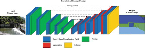
The encoder-decoder architecture is considered as the most efficient deep learning method for semantic segmentation in various fields, which is indicated in Figure 1. The encoder-decoder architecture views the backbone CNN as an encoder, responsible for encoding a raw input image into lower-resolution feature maps (e.g. $\frac{1}{m}$of input size,$m=8,16,32$). Afterwards, a decoder is utilized to recover the pixel-wise dense prediction from the lower-resolution feature maps. As to large-scale satellite images, the loss among down-sampling and up-sampling is non-negligible because of the limited receptive field.

Figure 1. SegNet architecture

To effectively alleviate the massive loss during training, DeepLab (Chen, Papandreou, and Kokkinos et al. 2018) uses atrous convolutions to enlarge the receptive field to extract contextual information comprehensively. Moreover, the enhanced version is duplicated then, termed as Deeplab v3+ (Chen, Zhu, Papandreou, et al. 2018). However, in these methods, the bilinear up-sampling is applied to obtain the desired pixel-wise prediction in decoders. Tian, He, and Shen et al. (2019) empirically verified that this over-simple and data-independent bilinear up-sampling might lead to sub-optimal results. Then DUsampling was proposed to use the redundancy in the label space of semantic segmentation. The relative encoder-decoder architecture makes the mIoU achieve 88.1% on PASCAL VOC dataset and 52.5% on PASCAL Context dataset.

Inspired by natural image semantic segmentation solutions, many targeted approaches, based on encoder-decoder networks, are designed for remote-sensing images. To acquire the desired accurate segmentation and localization, Zhang, Lin, and Ding et al. (2020) combined HRNet (High-resolution network) with ASP (Adaptive spatial pooling) to increase localization accuracy and preserve spatial details. The experimental results on the Vaihingen dataset (http://www2.isprs.org/commissions/comm3/wg4/2d-sem-label-vaihingen.html) and Potsdam dataset (http://www2.isprs.org/commissions/comm3/wg4/2d-sem-label-potsdam.html) reach SOTA. Ma, Wu, and Tang et al. (2020) designed a global and multi-scale encoder-decoder network to achieve building extraction of aerial images. The local and global encoder aims at learning the representative features from the aerial images for describing the buildings, while the distilling decoder focuses on exploring the multi-scale information for the final segmentation masks. Similarly, Keiller, Maruro, and Jocelyn et al. (2019) proposed a novel technique to perform semantic segmentation of remote sensing images that exploits a multi-context paradigm without increasing the number of parameters. And the experimental results show the same trend. Afterwards, U-Net (Su, Yang, and Jing 2019) is developed based on encoder-decoder architecture, which slightly improves the segmentation performance on remote-sensing data. Moreover, the recent proposed ResUNet-a (Foivos, François, and Peter et al. 2020) provides a reliable framework for the task of semantic segmentation of monotemporal very high-resolution aerial images. Furthermore, a remarkable fact is that the novel loss function based on the Dice loss is considerable. Apart from aerial images, a large-scale high-resolution dataset of GaoFen-2 satellite is available (http://captain.whu.edu.cn/GID). Simultaneously, Tong, Xia, and Shen et al. (2020) proposed a scheme to apply a deep transferable model to map the land-cover distributions. More recently, Zhao, Wang, and Wu et al. (2020) devised high accuracy algorithm by combining features expressed in different feature spaces with Riemannian manifold space and verified the effectiveness. To further explore spatial and channel dependencies of remote-sensing imagery, Li, Qiu, and Li et al. (2020) proposed a new end-to-end semantic segmentation network, which integrates two lightweight attention mechanisms that can refine features adaptively. Although the performance is excellent on ISPRS benchmarks, the application on large scale satellite images is unpredictable.

Unfortunately, there are two main urgent problems in semantic labelling high-resolution large-scale remote-sensing images:

1. The sub-optimal deep learning models: 1) in the existing methods, the utilization of abundant contextual information is insufficient. 2) Massive loss is produced which caused by data-independent bilinear up-sampling. During our empirical observation, the overfitting phenomenon occurs frequently. 3) Moreover, simplifying the deep learning model is still a pivotal task for practical application.

2. The imbalanced distribution of high-resolution large-scale remote-sensing images: Common models always ignore the imbalanced distribution, which leads to an increase of omissions and commissions. Thus the hard samples should be focus more during training. An optimal selection of loss function would boost the convergence and strengthen the model.

In order to tackle the aforementioned issues, a dual attention deep fusion semantic segmentation network of remote-sensing images (DASSN_RSI) is proposed, which enhances the extracted features in encoder stage, and fuses high-level features with low-level ones in lossless way in decoder stage. Additionally, a weight-adaptive focal loss (W-AFL) is designed to focus on hard samples during training, which further boosts convergence rate and reduces the total loss. Then our contributions can be summarized as follow:

1. A novel framework, named DASSN_RSI, is designed with encoder-decoder architecture. A dual attention mechanism (DAM), which embedded into the encoder stage, is proposed. More concretely, a shallow layer spatial attention module is incorporated to enhance the low-level feature extraction. Moreover, a deep layer channel attention module is incorporated to refine the high-level scale-invariance feature maps. Additionally, in decoder stage, the DUpsampling is introduced to flexible leveraging of almost arbitrary combinations of the features of the encoders. In this case, the decoder demonstrates less computation complexity without performance degradation.

2. A novel focal loss (FL) function, termed as weight-adaptive focal loss, is raised to boost the training process of proposed networks, leading to a higher convergence speed. Meanwhile, this loss function helps us focus more on the indeterminate samples, which explicitly decreases the training loss.

The rest of this paper is organized as follows. The preliminaries are introduced in section 2. Section 3 briefly explains the proposed method that contains framework and the modified loss function. The experimental results are presented in section 4. The conclusions and future works are discussed in section 5.

2. Preliminaries

2.1. Encoder-decoder architecture

As shown in Figure 1, the details of a symmetric encoder-decoder network named SegNet is demonstrated. The architecture of the encoder network is topologically identical to the 13 convolutional layers in the VGG16 network (Simonyan 2015). Then the decoder stage aims to map the encoder feature maps to the same resolution feature maps with raw input for pixel-wise classification. The novelty of SegNet lies in the manner in which the decoder up-samples the lower resolution feature maps. Notably, the pooling indices computed in the max-pooling step are selected to perform non-linear up-sampling. Finally, the up-sampled maps are sparse and convolved with trainable filters to produce dense predictions.

This architecture successfully performs robustness in many other scenarios, while starting with the road and indoor scene understanding. Notably, the encoder phase is adopted as the backbone in proposed networks.

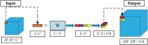
2.2. DUpsampling in decoders

As illustrated in Figure 2, the details of DUpsampling (Tian, He, and Shen et al. 2019) operation is presented. A pixel in lower resolution can be relatively inferred to a region in a higher resolution feature map.

Figure 2. DUpsampling operation

Please put Figure 2 about here

Let $F_{\mathrm{D}\mathrm{I}}$denotes the final output of the encoder, with a factor (16 or 32) in the spatial size of the ground-truth $GT$, and $F_{DI}\in {\mathbb{R}}^{\tilde{H}\times \tilde{W}\times \tilde{C}}$. $GT$ denotes the label of an image. Notably, we assume that $GT$ can be compressed without loss. $GT$ is normally encoded with one-hot encoding, i.e., $\mathrm{G}\mathrm{T}\in {\left\{0,1\right\}}^{H\times W\times C}$. Thus we can see $\frac{\tilde{H}}{H}=\frac{\tilde{W}}{W}=\frac{1}{16}or\frac{1}{32}$. And $F_{DI}$ needs to be up-sampled to the spatial size of $GT$ before computing training loss. Here we present the original loss function based on the cross-entropy (CE) loss. The formulation is as follows,

(1) $L(F_{\mathrm{D}\mathrm{I}},GT)=L(\mathrm{s}\mathrm{o}\mathrm{f}\mathrm{t}\mathrm{m}\mathrm{a}\mathrm{x}(\mathrm{B}\mathrm{i}\mathrm{l}\mathrm{i}\mathrm{n}\mathrm{e}\mathrm{a}\mathrm{r}(F_{\mathrm{D}\mathrm{I}})),GT)$(1)

where $L$denotes the loss function, $\mathrm{B}\mathrm{i}\mathrm{l}\mathrm{i}\mathrm{n}\mathrm{e}\mathrm{a}\mathrm{r}(F_{\mathrm{D}\mathrm{I}})$represents the bilinear up-sampling. As to DUpsampling, the loss function can be denoted as follows,

(2) $L(F_{\mathrm{D}\mathrm{I}},GT)=L(\mathrm{s}\mathrm{o}\mathrm{f}\mathrm{t}\mathrm{m}\mathrm{a}\mathrm{x}(\mathrm{D}\mathrm{U}\mathrm{p}\mathrm{s}\mathrm{a}\mathrm{m}\mathrm{p}\mathrm{l}\mathrm{e}(F_{\mathrm{D}\mathrm{I}})),GT)$(2)

An important observation is that the semantic segmentation label $GT$ is not i.i.d. and there contains structure information so that $GT$ can be compressed considerably, with almost no loss. Hence, the authors compress $GT$ into $\widetilde{GT}\in {\mathbb{R}}^{\tilde{H}\times \tilde{W}\times \tilde{C}}$and then compute the training loss between $F_{\mathrm{D}\mathrm{I}}$ and $\widetilde{GT}$. Obviously, $F_{\mathrm{D}\mathrm{I}}$keeps the same spatial size with $\widetilde{GT}$.

So the key problem is the compression from $GT$ to $\widetilde{GT}$. Let$r$indicate the ratio of $H$to$\tilde{H}$. Afterwards, $GT$is divided into an $\frac{H}{s}\times \frac{W}{s}$grid of each sub-window of size$\mathrm{s}\times s$(padding if $H$or $W$is undivided). For each sub-windows$S\in {\left\{0,1\right\}}^{\mathrm{s}\times s\times C}$, it can be reshaped to a vector $v={\left\{0,1\right\}}^N$, $N=s\times s\times C$. Finally, the vector $v$is compressed to $x\in {\mathbb{R}}^{\tilde{C}}$, so $\widetilde{GT}$can be vertically and horizontally obtained by stacking all $x\in {\mathbb{R}}^{\tilde{C}}$. Formally,

(3) $x=\mathbf{P}v;\tilde{v}=\mathbf{W}x$(3)

where $\mathbf{P}\in {\mathbb{R}}^{\tilde{C}\times N}$is used to compress$v$to$x$, $\mathbf{W}\in {\mathbb{R}}^{N\times \tilde{C}}$is used to generate $v$, $\tilde{v}$ is reformed$v$. The matrices $\mathbf{P}$ and $\mathbf{W}$ can be found by minimizing the error between $v$ and $\tilde{v}$ over the training set. Formally,

(4) $\begin{array}{rl}& {\mathbf{P}}^{\ast },{\mathbf{W}}^{\ast }=\underset{\mathbf{P},\mathbf{W}}{\mathrm{a}\mathrm{r}\mathrm{g}\mathrm{m}\mathrm{i}\mathrm{n}}\sum _v{∥v-\tilde{v}∥}^2\\ & =\underset{\mathbf{P},\mathbf{W}}{\mathrm{a}\mathrm{r}\mathrm{g}\mathrm{m}\mathrm{i}\mathrm{n}}\sum _v{∥v-\tilde{v}∥}^2\\ & =\underset{\mathbf{P},\mathbf{W}}{\mathrm{a}\mathrm{r}\mathrm{g}\mathrm{m}\mathrm{i}\mathrm{n}}\sum _v{∥v-\mathbf{W}\mathbf{P}v∥}^2\end{array}$(4)

This objective can be iteratively optimized with standard stochastic gradient descent (SGD). With an orthogonality constraint, we can simply use principal component analysis (PCA) (Wold, Esbensen, and Geladi 1987) to achieve a closed-form solution for the objective.

Using $\widetilde{GT}$ as the target, they pre-train the network with a regression loss by observing that the compressed labels $\widetilde{GT}$ is the real-valued,

(5) $L(F_{\mathrm{D}\mathrm{I}},GT)={∥F_{\mathrm{D}\mathrm{I}}-\widetilde{GT}∥}^2$(5)

Therefore, instead of compressing $GT$ to $\widetilde{GT}$, they up-sample $F_{\mathrm{D}\mathrm{I}}$ with the learned reconstruction matrix $\mathbf{W}$. Finally, the pixel classification loss is computed as Equation (2)(2) $L(F_{\mathrm{D}\mathrm{I}},GT)=L(\mathrm{s}\mathrm{o}\mathrm{f}\mathrm{t}\mathrm{m}\mathrm{a}\mathrm{x}(\mathrm{D}\mathrm{U}\mathrm{p}\mathrm{s}\mathrm{a}\mathrm{m}\mathrm{p}\mathrm{l}\mathrm{e}(F_{\mathrm{D}\mathrm{I}})),GT)$(2) .

As indicated in (Tian, He, and Shen et al. 2019), DUpsampling significantly reduces the computation time and memory footprint of the semantic segmentation method by a factor of 3 or so. Besides, DUpsampling also allows a better feature aggregation to be exploited in the decoder by enlarging the design space of feature aggregation.

2.3. Attention mechanism

The attention mechanism is well known because of its significant position in human perception (Itti, Koch, and Niebur 1998; Maurizio and Gordon 2002). To our analysis, the human visual system does not attempt to process a whole scene at once. Instead, humans exploit a sequence of partial glimpses and selectively focus on salient parts. This property makes the human perception capture visual information better.

Latterly, there have been several attempts to incorporate attention processing to improve the performance of CNNs in large-scale classification tasks (Wang, Wang, and Zhang et al. 2017; Hu, Li, Samuel, et al. 2020; Li, Li, and He et al. 2020). Wang, Jiang, and Qian et al. (2017) proposed a residual attention network which refines the feature maps. And the extensive experiments verify the less computational and parameter overhead. After that, a squeeze-and-excitation (SE) block was developed in (Hu, Li, and Samuel et al. 2020), which explicitly models the inter-dependencies across discriminative channels. Then the channel-wise feature maps can be recalibrated. However, they miss the spatial attention, which plays a significant role in deciding ‘where’ to focus. Specifically, the remote-sensing images processing involves massive inter-channel and intra-channel dependencies. To fulfill this requirement, we suppose to design an attention mechanism, which incorporates the spatial attention module and channel attention module.

3. Method

3.1. Framework overview

In this part, we first illustrate the whole architecture of our proposed DASSN_RSI. As show in Figure 3, the encoder-decoder architecture is explicitly expressed.

Figure 3. Overview of proposed framework

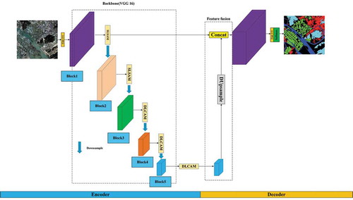
To our analysis, we define the feature extracted from the 3rd block (the block marked in green) is high-level feature. Thus the SLSAM and DLCAM are incorporated in the corresponding positions. In decoder stage, the main feature fusion operation is composed by concatenating the up-sampled semantic features with the low-level features that keep the same resolution with raw images. Finally, the semantic segmentation results are obtained by a simple convolutional layer followed by a softmax layer.

In large-scale satellite images, it is essential to learn the relationship between different blocks on a channel and model the relationship of semantic information on different channel images. However, because convolution extracts feature through fixed-size local receptive fields, it is difficult to simultaneously consider local and global information. To solve this problem, we introduce two attention modules to capture the spatial and channel dependencies between any two positions of the feature maps and between any two channel maps, respectively.

Individually, a raw input image is firstly convolved to collect spatial feature maps. Then the refined spatial feature maps are extracted by SLSAM during the first two blocks. In deeper layers, the raw image is willing to down-sampled to obtain refined high-level semantic feature maps after DLCAM. Finally, the refined high-level semantic features are DUpsampled to original spatial resolution and fused with refined low-level spatial details for final dense prediction. From whole sight, the up-sample matrix is automatically learned and fine-tuned during the end-to-end training.

Notice that, the blocks with different colour denote different spatial resolution, and the five blocks contain the same processing refer to SegNet. The next parts are going to explain the network architecture and the applicable principles detailedly.

3.2. Shallow layer spatial attention module

In this section, the shallow layer spatial attention module is specified. As demonstrated in Figure 4, since the convolution of the encoder stage can only model local features, it cannot model a more extensive range of spatial relationships. The low-level features, which extracted from shallow layers, contain complementary spatial structural details and objects’ boundaries. Notably, this property will guide the segmentation in the decoder stage. For example, the clear river boundaries improve the segmentation performance of river areas. Next, we elaborate the process to adaptively aggregate spatial contexts.

Figure 4. Details of SLSAM

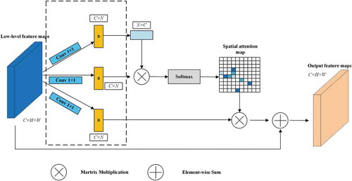
As can be seen in Figure 4, the self-attention mechanism is selected to emphasize the spatial dependencies between any two positions of the feature maps. Let the input feature maps denoted as $S{A}_{int}\in {\mathbb{R}}^{C\times H\times W}$, then three identical feature maps $S{A}_B\in {\mathbb{R}}^{C\times H\times W}$are obtained through three convolution layers. A reshape operation is subsequently applied to the first branch following by a matrix multiplication between the reshaped feature map with un-reshaped ones. The next softmax layer is opted to calculate the spatial attention map $\mathbf{M}\in {\mathbb{R}}^{N\times N}$:

(6) ${\mathbf{M}}_{j,i}=\frac{exp({\left(S{A}_B\right)}_i\times {\left(S{A}_B\right)}_j)}{{\sum }_{i=1}^{N}exp({\left(S{A}_B\right)}_i\times {\left(S{A}_B\right)}_j)}$(6)

where ${\mathbf{M}}_{j,i}$ indicates the impact on$j^{th}$position from $i^{th}$, $i$and$j$denotes the position in feature map. Afterwards, the transposed $\mathbf{M}$ is matrix multiplication with $S{A}_B$. Then the result could be reshaped to ${\mathbb{R}}^{C\times H\times W}$. Finally, the value of$j^{th}$position in output refined feature maps is calculated as follows:

(7) ${\left(S{A}_o\right)}_j=\alpha {\sum }_{i=1}^N({\mathbf{M}}_{j,i}{\left(S{A}_B\right)}_i)+{\left(S{A}_{int}\right)}_j$(7)

where $\alpha$is initialized to 0 and gradually learns to assign more weight, $S{A}_o$denotes the output feature maps, $j$ indicates a position in the feature map. For example, the value of $j^{th}$ position in output feature map is calculated by the sum of the ${\mathbf{M}}_{j,i}$ of other positions and the $j^{th}$ value in$S{A}_{int}$. Concretely, it can be inferred from Equation (7)(7) ${\left(S{A}_o\right)}_j=\alpha {\sum }_{i=1}^N({\mathbf{M}}_{j,i}{\left(S{A}_B\right)}_i)+{\left(S{A}_{int}\right)}_j$(7) that the resulting feature $S{A}_o$ at each position is a weighted sum of the features across all positions and original features. Therefore, it has a global contextual view and selectively aggregates contexts according to the spatial attention map. The similar semantic features achieve mutual gains, thus improving intra-class compact and semantic consistency. Through the SLSAM, a weighted sum of the features across all elements’ positions and the raw features is supposed to be the refined feature maps.

3.3. Deep layer channel attention module

In this section, the designed DLCAM, which is applied to enhance the high-level semantic feature maps (see Figure 5), is introduced. Generally, this module exploiting the inter-channel relationship of features. As each channel of a feature map is considered as a feature detector, channel attention focuses on ‘what’ is meaningful given an input image. Notably, we present an enhancement of semantic correlation across different channels. As we know, high-level features contain global context-aware semantic information, which is pivotal in instructing the segmentation. Besides, we embed this module following three deep blocks to achieve a consideration of multi-scale semantic information.

Figure 5. Details of DLCAM

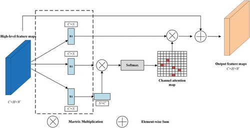
As vividly depicted in Figure 5, the DLCAM is presented to apprehend channel-wise correlations and dependencies. Similarly, the objective of this structure designation is to refine the input feature maps. In the beginning, the 1 × 1 convolution layer is removed. This is because that the utilization of convolution operation might break the original mapping relationships across channels.

For the further expression of DLCAM, let the input high-level features denoted as $C{A}_i\in {\mathbb{R}}^{C\times H\times W}$, different from SLSAM, the convolution layer is unnecessary. Because the introduction of convolution operation could break the original mapping relationships across channels. $C{A}_i\in {\mathbb{R}}^{C\times H\times W}$is directly reshaped to $C{A}_B\in {\mathbb{R}}^{C\times N}$,where $N=H\times W$, which indicates the number of pixels. Similarly, after the application of matrix multiplication and softmax layer, the channel attention map is formed as:

(8) $C{A}_{j,i}=\frac{exp({\left(C{A}_B\right)}_i\times {\left(C{A}_B\right)}_j)}{{\sum }_{i=1}^{C}exp({\left(C{A}_B\right)}_i\times {\left(C{A}_B\right)}_j)}$(8)

where $C{A}_{j,i}$ represents the channel-wise correlation between $i$ and $j$. Then the final output refined features are obtained by a matrix multiplication processing and element-wise sum operation, which can be defined as bellow,

(9) $C{A}_o=\beta {\sum }_{i=1}^C(C{A}_{j,i}\times {\left(C{A}_B\right)}_i)+{\left(C{A}_i\right)}_j$(9)

where $\beta$ is a similar weight factor with$\alpha$.

In a word, the DLCAM provides a wider range of semantic correlations between different high-level feature maps. As a result, the refined features are more discriminative.

3.4. Weight-adaptive focal loss

In this section, we are going to explain the details of proposed weight-adaptive focal loss function (W-AFL), which aims to further boost the convergence rate of the networks and improve the semantic segmentation performance.

As we comprehend, the loss function is designed to minimize the training loss to produce an optimal model. The aforementioned methods commonly utilize the CE loss to perform semantic segmentation networks. However, for large-scale satellite remote-sensing images, the unbalanced distribution is particularly prominent. We should pay more attention to hard examples, which always manifests discrete distribution and negative learning efficiency.

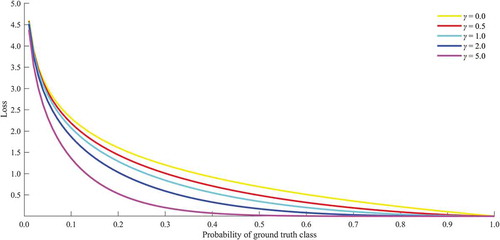
Focal loss is proposed to promote dense detectors in literature (Lin, Priya, and Ross et al. 2020). Inspired by the substantial ability to focus on hard samples, we creatively modify the focal loss function to intensively centre the mutual influence between unbalanced-class and complex land-cover diversities. The original focal loss is defined as below:

(10) $p_t=\left\{\begin{array}{c}p\hspace{0.17em}ify=1\\ 1-p\hspace{0.17em}otherwise\end{array}\right.$(10)

(11) $\mathrm{F}\mathrm{L}(p_t)=-{\left(1-p_t\right)}^{\gamma }log\left(p_t\right)$(11)

where $y\in \left\{\pm 1\right\}$specifies the ground truth class and $p\in \left[0,1\right]$is the model’s estimated probability for the class with label$y=1$. For notation convenience, $p_t$is defined as before. When $\gamma =0$the focal loss is turned to CE loss.

Visually, as can be seen in Figure 6, the curves are drawn with the different parameters of$\gamma$. In large-scale satellite images, a notable property of focal loss is that even easily classified samples provoke a loss with non-trivial magnitude. Because these small losses couldn’t be ignored when summed over a large number of pixels. The massive class imbalance encountered during the training of multi-class dense classification overwhelmingly increase the loss. Easily classified negatives comprise the majority of the loss and dominate the gradient. To overcome this problem, we propose to modify the focal loss function to down-weight easy samples and focus on hard samples, which is formed as follows,

(12) $\mathrm{W}-\mathrm{A}\mathrm{F}\mathrm{L}(p_t)=-\epsilon {\left(1-p_t\right)}^{\gamma }log\left(p_t\right)$(12)

Figure 6. Illustration of focal loss

where $\epsilon$ represents the balance factor. In the presence of class imbalance, the loss due to the frequent class can dominate total loss and cause instability in early training. To counter this, we introduce the concept of a ‘prior’ which is estimated by the model for the rare class of the input data. Therefore, the balance factor $\epsilon$is introduced into the focal loss function.

Automatically, the balance factor is computed by a simple prior distribution of a training raw image. Let the total class number be$N_C$, thus$\epsilon$can be denoted as follows,

(13) $\epsilon =\sum _{i=1}^{N_C}\frac{1-\frac{N_{p,i}}{N_p}}{N_C+1}$(13)

Respectively, $N_{p,i}$denotes the pixels of $i^{th}$class, $N_p$denotes the total pixels of a raw input image. Instead of handcraft settings, the dynamic balance factor is generalized adaptive. Prominently, this modification yields improvement accuracy slightly with the original ones. Because the networks are dynamically paying more attention to hard samples.

3.5. Attention module embedding with Networks

Primarily, the whole network is end-to-end. The parameters, include the SLSAM module, DLCAM module, and DUpsampling. As indicated before, the backbone of the encoder stage is VGG16, which is the same with SegNet, U-Net, and ResUNet – a. On this basis, SLSAM and DLCAM modules are incorporated with related layers. In SCAttNet (spatial and channel attention mechanism), the dual attention module is embedded at the end of the encoder, refining the final feature maps of the encoder. To take full advantage of long-range contextual information, we propose to aggregate the features from refined shallow layers’ feature maps with high-level semantic features. Specifically, we transform the outputs of two attention modules by a convolution layer and perform an element-wise sum to accomplish feature fusion. At last, a convolution layer is followed to generate the final prediction map. We do not adopt a cascading operation because it needs more GPU memory. Noted that our attention modules are simple and can be directly inserted in the existing FCN pipeline. They do not increase too many parameters yet strengthen feature representations effectively.

4. Experimental results

4.1. Datasets

Tong, Xia, and Shen et al. (2020) construct a large-scale land-cover dataset with Gaofen-2 satellite images. GID dataset contains large-scale high-resolution satellite images (3.2 m spatial-resolution) and the corresponding well-annotated label images. This dataset consists of two parts: a large-scale classification set (GID-C) and a fine classification set (GID-F). The former set has 150 pixel-level annotated Gaofen-2 images, and the latter one is composed of 30,000 multi-scale image patches coupled with ten pixel-level annotated Gaofen-2 images. More details are presented in the Table 1. Figure 7 displays the partial samples of the large-scale classification set with five categories. Figure 8 manifests a refined set with 15 categories.

Table 1. GID dataset

Set	GID-C	GID-F
Labelled classes	5	15
Data size (number of images)	150	10
Spatial size per image	6800 × 7200 × 4	6800 × 7200 × 4
Number of bands	4	4
Spatial resolution (m)	3.2	3.2

Figure 7. Examples of GID-C dataset, (a) Original image, (b) Ground truth

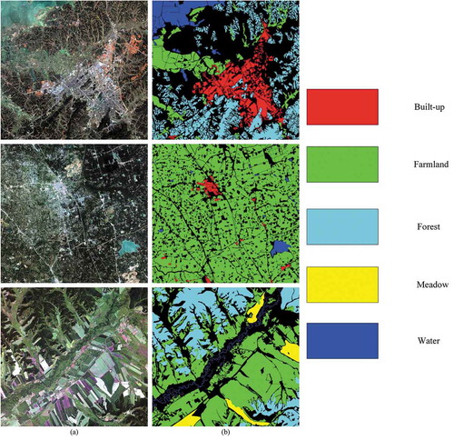
Figure 8. Examples of GID-E dataset, (a) Original image, (b) Ground truth

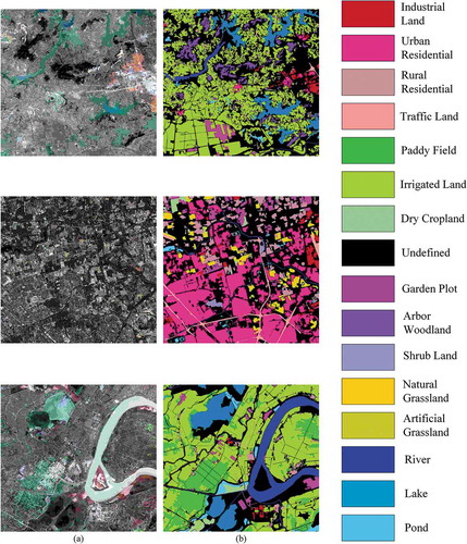
Based on the GID-F dataset, the expanded fine classification dataset (GID-E) is introduced with more sample images with ground truth label, which acquired randomly, covering wider range of China along with the Yellow River basin. GID-E is double size than before, which contains 20 images with annotated label images (15 categories). This contribution provides the dataset more diverse, making the trained model has stronger generalization.

4.2. Implement details

The proposed method is implemented based on the ‘Tensorflow (TF)’ deep learning framework. The experimental environment is a PC with Intel i7-8750 H CPU, 32GB of memory, and the NVIDIA Geforce 1080Ti (8GB).

For the training stage, the ‘poly’ learning rate policy is selected referring to (Chen, Papandreou, and Kokkinos et al. 2018). As can be seen in Equation (14)(14) $\mathrm{L}\mathrm{R}=({\mathrm{L}\mathrm{R})}_{\mathrm{i}\mathrm{n}\mathrm{t}}\times {\left(1-\frac{N}{N_{max}}\right)}^{0.9}$(14) , the learning rate is scheduled by multiplying a decaying factor to the initial learning rate. As listed in Table 2, the initial learning rate and weight decay is 0.007 and 0.0001. Notably, the adaptive temperature softmax is directly incorporated into the framework encounters difficulties in optimization (Hinton, Vinyals, and Dean 2015).

(14) $\mathrm{L}\mathrm{R}=({\mathrm{L}\mathrm{R})}_{\mathrm{i}\mathrm{n}\mathrm{t}}\times {\left(1-\frac{N}{N_{max}}\right)}^{0.9}$(14)

Table 2. Settings of hyper-parameters

Hyper-parameter	GID-C	GID-E
Categories	5	15
Training (number of images)	120	16
Validation (number of images)	15	2
Test (number of images)	15	2
Patch size	400 × 400 × 4	400 × 400 × 4
Batch size	8	8
Max epoch	200	200
Initial learning rate	0.007	0.007
Weight decay	0.0001	0.0001

where $\mathrm{L}\mathrm{R}$denotes the learning rate and ${(\mathrm{L}\mathrm{R})}_{\mathrm{i}\mathrm{n}\mathrm{t}}$indicates the initial learning rate, $N$is the current number of epoch, and $N_{max}$is the max epoch number.

In order to achieve a status of steady convergence, we set the max-epoch as 200. During training phase, the raw input is split to many patches with a spatial resolution of 400 × 400 × 4, and the batch size is 8 (could be bigger with more powerful devices). The details of hyper-parameters are listed in Table 2. The ratio of training set, validation set and test set is 8:1:1, which is a balanced partition refer to the expertise and data properties.

4.3. Evaluation metrics

For each tile of the test set, we form the confusion matrix and extract average accuracy (AA), the $F_1$-score ($F_1$), and the mean of class-wise intersection over union (mIoU). The equations are as below.

(15)) $\mathrm{A}\mathrm{A}=\frac{\left(\mathrm{T}\mathrm{P}\right)+(\mathrm{T}\mathrm{N})}{(\mathrm{T}\mathrm{P})+(\mathrm{F}\mathrm{P})+(\mathrm{F}\mathrm{N})+(\mathrm{T}\mathrm{N})}$(15))

(16) $F_1=\frac{2\times P\times R}{\left(P+R\right)}$(16)

(17) $P=\frac{(\mathrm{T}\mathrm{P})}{\left(\mathrm{T}\mathrm{P}\right)+(\mathrm{F}\mathrm{P})}$(17)

(18) $R=\frac{(\mathrm{T}\mathrm{P})}{\left(\mathrm{T}\mathrm{P}\right)+(\mathrm{F}\mathrm{N})}$(18)

(19) $\mathrm{m}\mathrm{I}\mathrm{o}\mathrm{U}=\frac{(\mathrm{T}\mathrm{P})}{(\mathrm{T}\mathrm{P})+(\mathrm{F}\mathrm{P})+(\mathrm{F}\mathrm{N})}$(19)

where TP denotes the number of true positives, FP denotes the number of true positives, FN denotes the number of false negatives, TN denotes the number of true negatives, P indicates the precision, and R for recall.

Accordingly, the precision for a class is the number of true positives (i.e. the number of items correctly labelled as belonging to the positive class) divided by the total number of elements labelled as belonging to the positive class (i.e. the sum of true positives and false positives, which are items incorrectly labelled as belonging to the class). Recall is defined as the number of true positives divided by the total number of elements that actually belong to the positive class (i.e. the sum of true positives and false negatives, which are items which were not labelled as belonging to the positive class but should have been). F₁ is the combination of precision and recall. F₁ and mIoU are the major evaluation metrics that directly reflect the performance of a model. mIoU is the mean of class-wise intersection over union on each category, commonly used in both natural and remote-sensing image semantic segmentation.

4.4. Comparisons on GID-C

To comprehensively evaluate the method, extensive comparative experiments are conducted on GID-C dataset. And several mainstream methods based on encoder-decoder architecture are implemented, include SegNet (Badrinarayanan et al. 2017), U-Net (Su, Yang, and Jing 2019), SCAttNet (Li, Li, and He et al. 2020), and ResUNet-a (Foivos, François, and Peter et al. 2020). The results presented in Table 3 are a class-wise average of test data (see Table 2).

Table 3. Numerical evaluation on GID-C (%)

Method	P	R	F1	AA	mIoU
SegNet	0.7855	0.7414	0.7628	0.7628	0.6166
U-Net	0.8546	0.7723	0.8114	0.8107	0.6826
SCAttNet	0.8153	0.8676	0.8407	0.8398	0.7252
ResUNet-a	0.8607	0.8118	0.8355	0.8366	0.7175
Ours	0.8749	0.8332	0.8537	0.8549	0.7445

Generally, the proposed DASSN_RSI achieves the best performance among other encoder-decoder semantic segmentation networks. Meanwhile, with the incorporation of the attention mechanism, SCAttNet and DASSN_RSI, produces excellent performance than others. We speculate about the leading cause is that the adaptively refined feature maps by attention mechanism maintain critical contextual information, including semantical and spatial details. The highest value of mIoU of DASSN_RSI, which is increased by more than 10% versus SegNet, reflects that this method can make the accurate pixel-wise classification and localization to a large extent. U-Net partially alleviates the lack of correctly labelled data by transposing more details for up-sampling. Peculiarly, the concatenation operation is incorporated to realize a sharper recovered image. Thus F₁ value and AA are slightly improved by about 2% and 4%, while mIoU grows to more than 68%. With the introduction of atrous convolutions, pyramid scene parsing pooling, and multi-tasking inference, the ResUNet-a achieves the SOTA performance with more than 71% of mIoU. This improvement also arises from the amelioration of dice loss, which has excellent convergence properties and behaves well even under the presence of highly imbalanced classes. Instead of introducing atrous convolutions, dual attention mechanism and DUpsampling are supposed to be a lightweight fashion. And the accuracy performance is better than ResUNet-a on large-scale satellite images. With the factual proof, the refined feature maps by attention mechanism are essential to produce representations. Meanwhile, the DASSN_RSI is much lower computational than ResUNet-a.

Besides, the DUpsampling boosts the convergence while maintaining lossless, and simplifying the steps in decoder phase. On the whole, the F₁ score, AA and mIoU of DASSN_RSI are higher than SCAttNet, due to the adequately deep fusion of the refined low-level feature maps, which have massive spatial details. In contrast, the SCAttNet ignores the shallow layers’ feature maps. Another reason for the slight improvement derives from the W-AFL is tuning the loss with consideration of class-imbalance distribution. The detailed IoU of each category of GID-C test set is discussed in the supplemental material.

In addition to numerical evaluation, visual inspection is necessary to prove the capability further. As depicted in Figure 9, a random test image is selected to perform semantic segmentation. From an overall perspective, the results are discriminative, and the negative impacts of hard samples are suppressed. The visual inspection keeps the same trend with numerical evaluation. The key objects in a large-scale satellite image are essentially delineated by our method, while cannot be captured by others. Typically, two areas are featured in the results, containing the low-ratio distributional pixels of the whole images. From Figure 9 (c) and 9 (d), the results are coarse. Mainly, there are lots of omissions, because these two methods cannot handle the hard samples, which directly lead to the uncertainty of classifier. From Figure 9 (e), ResUNet-a generally labels the central area of forest and farmland. Yet it is incomplete. The drawback might lie in the loss function, which equally treats the samples. As presented in Figure 9 (g), the segmentation result almost overlaps with the ground truth, which stands for a high consistency with ground truth. The water areas are extracted well, due to the essential different with other categories. And the indistinguishable multi-scale built-up and forest objects are ultimately outlined in the white squares.

Figure 9. Results on GID-C test set, (a) Original image, (b) Ground truth, (c) SegNet, (d) U-Net, (e) ResUNet-a, (f) SCAttNet, (g) Ours

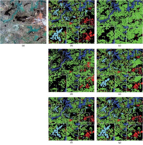
Although ResUNet-a performs well at semantic segmentation of these two areas. The dual attention-based methods express the potential in refining feature representations and recovering dense predictions – however, the different combinations of dual attention mechanism exhibits heterogeneous performance. The spatial details of shallow layers, which are ignored in SCAttNet, are also crucial for segmentation. That’s why we get better results, including a more smooth boundary and higher consistency. It means that the imbalanced distrubution problem is effectively solved.

In conclusion, DASSN_RSI reaches SOTA in many quantitative indicators. And the visual inspection verifies it. Whether it is an easy or hard sample pixel with an irregular distribution, DASSN_RSI can effectively accomplish a well-made result than other variants of encoder-decoder networks.

4.5. Comparisons on GID-E

Facing with a five categories’ dense prediction task, DASSN_RSI achieves the SOTA performance in both numerical evaluation and visual inspection. The multi-scale samples in raw images are targeted and refined, which directly affects final predictions. A more formidable task (15 categories’ objects) is posed to assess the robustness of existing semantic segmentation networks.

As can be seen in Table 4, the numerical values of SCAttNet and DASSN_RSI are generally superior to others. Each method has a declined performance resulting from the tougher goal. Taking SegNet as an example, the mIoU drops down to less than 55%. However, the mIoU of DASSN_RSI decreases by about 3%. Due to the introduction of dual attention mechanisms, the spatial details and semantic features are refined to provide much more clues for dense prediction. Thus the proposal expresses the strongest generalization than others with different levels of the task. An alternative reason is the fine-tuning by W-AFL, which is beneficial to every category whether the distribution is balanced or not. The average accuracy and average class-wise F₁ reaches almost 84% and more than 83%. Moreover, the detailed IoU of each category of GID-E test set is discussed in the supplemental material.

Table 4. Numerical evaluation on GID-E (%)

Method	P	R	F1	AA	mIoU
SegNet	0.7277	0.6902	0.7085	0.7229	0.5485
U-Net	0.7721	0.7257	0.7482	0.7511	0.5977
SCAttNet	0.7898	0.7993	0.7945	0.8008	0.6591
ResUNet-a	0.7982	0.7720	0.7849	0.7802	0.6460
Ours	0.8370	0.8276	0.8323	0.8393	0.7129

Similarly, visual inspection is presented in Figure 10. The test images are labelled by multiple comparative methods. Reputably, in the areas marked with red lines, the fundamental objects are accurately extracted by ours, while others are undesirable. Owing to the confusable of river, lake, and pond, which belongs to water, SegNet and U-Net cannot distinguish and label them. Although the ResUNet-a is more salutary, the results are useless. The attention mechanism helps the network pay more attention to inter-class objects with higher similarities. Furthermore, with the auxiliary W-AFL, discrimination is emphasized by the refined feature vectors. Thus, DASSN_RSI, which combines DAM with W-AFL, effectively addresses this problem by paying more attention to these less distinguishable pixels. In Figure 10 (g), the desired results are acted. In the bottom rectangular region, the urban residential, rural residential, industrial land, and traffic land areas are nearby. The segmentation of SegNet (see Figure 10 (c)) and U-net (see Figure 10 (d)) is insufficient. There are lots of blurs, while labels are clear. ResUNet-a achieves improvements with regard to loss function and multi-residual learning strategy. Surpassingly, the most similar results are obtained by our approach. The sharp boundaries and fewer blurs are illustrated.

Figure 10. Results on GID-E test set, (a) Original image, (b) Ground truth, (c) SegNet, (d) U-Net, (e) ResUNet-a, (f) SCAttNet, (g) Ours

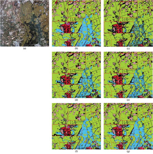
To be briefly, DASSN_RSI shows vast generalization and robustness in multiple semantic segmentation tasks, whether the number of categories. Accordingly, this superiority provides the possibility of a broader application.

4.6. Ablation study of dual attention mechanism

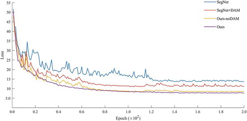
In this part, the extensive ablation study of the dual attention mechanism is conducted. Due to the flexibility of embedding, four alternative methods are realized, which provides available comparable results of training loss. In experiments, we implement SegNet and a dual attention version of SegNet, DASSN_RSI and a no dual attention version of DASSN_RSI on GID-C dataset.

The intuitive performance is illustrated in Figure 11, in which the relationship between training loss and epochs is entirely presented. A prominent improvement rests on the reduction of loss. The training loss of the original SegNet is about 13.69, while the DAM version is 11.10, which significantly decreases by 19%. Likewise, the training loss of no DAM version with the proposed architecture increases on average of 0.75. Besides, the convergence rate is boosted by the incorporation of DAM, whether the backbone is SegNet or ours. Accordingly, the convergence status of our approach is more stable than before, which auxiliary evidence the superior upper bound performance.

Figure 11. Training loss with different architecture

4.7. Ablation study of loss function

This part discusses the ablation study of the loss function in our approach. As indicated previously, W-AFL is inferred and explained, which could significantly boost the convergence rate and minimize the total loss during training. The balance factor further helps the focal loss function to fine-tune the classification of hard samples. Instead of handcraft, the balance factor’s ($\epsilon$) value is adaptively calculated by the raw input data.

To effectively evaluate the option of the loss function, cross-entropy loss, focal loss, and weight-adaptive focal loss are embedded and trained based on the proposed framework. The training accuracy with epochs is demonstrated in Figure 12. The FL-based training strategy makes the network lossless than CE loss, which equally treats the imbalanced class pixels. At convergent status, the training accuracy still much lower with CE. The omissions and commissions might be a small part of images, yet the account errors are non-negligible.

Figure 12. Training accuracy with different loss function

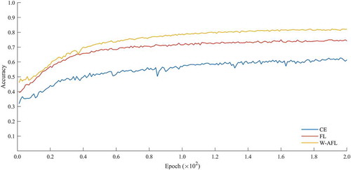
In contrast, FL adapts to these surroundings more. The training accuracy and convergence rate is significantly increased. Furthermore, the W-AFL slightly enhances the network’s capability than the original FL, while the computational complexity keeps the same magnitude.

4.8. Inference time comparison

In this part, the comparison of inference time is manifested. As to practical application, efficiency is essential. Thus a single input image with a spatial size of 6800 × 7200 is opted to test the execution time. Based on the pre-trained model, the inference time is listed in Table 5. During the test, the environment settings are fixed to ensure the reliability of results.

Table 5. Execution time comparison

Model	Execution time (×10^2 s)
SegNet	1.0657
U-Net	1.0576
SCAttNet	0.8955
ResUNet-a	1.0198
Ours	0.8723

Generally, as can be seen in Table 5, all encoder-decoder networks express positive performance in inferring a test image. Compared with SegNet, U-Net slightly improves inference efficiency. Moreover, ResUNet-a further enhances the processing speed with significant improvement than SegNet. Similarly, the lightweight SCAttNet also boost the inference efficiency with less matrix multiplications. Among them, the proposed DASSN_RSI takes the least time to finish the raw input image’s semantic segmentation task. Intuitively, the multiple up-sampling operations are removed, which provides a marked reduction of time costs.

4.9. Training time comparison

In this part, the comparison of training time is manifested. Table 6 presents the training time per epoch, which directly derived from the model size, network parameters, and size of training set. We implement comparative methods under the ‘Tensorflow’ framework for fairness.

Table 6. Training time per epoch (×10³ s)

Model	GID-C training set	GID-E training set
SegNet	1.493	0.112
U-Net	1.827	0.126
SCAttNet	1.689	0.133
ResUNet-a	2.976	0.192
Ours	1.622	0.122

As can be seen in Table 6, the training time per epoch is automatically monitored and recorded. In general, the GID-C training set needs much more time than GID-E. This result is caused by the size of the training set, in which GID-C has more than ten times of images than GID-E. Under the same environments and parameters, the proposed method expresses potential performance in training time costs, which are slightly more than the SegNet baseline. ResUNet – a achieves state-of-the-art while sacrificing massive efficiency with the complex network architecture. Notably, the lightweight SCAttNet needs more training time than ours and U-Net. And the prominent reason that we infer arise from the decoder stage, in which multiple matrix multiplications and convolutions are replaced by unique DUpsampling. Overall, the proposed method balances efficiency and performance well.

5. Conclusion

This paper comprehensively analysed the drawbacks of the existing semantic segmentation methods of remote-sensing images. Although deep neural networks provide a promising performance, the insufficient utilization of contextual information extremely limits the application of large-scale satellite images.

On this basis, a dual attention semantic segmentation network of remote-sensing images is proposed. Our proposal effectively extracts and refines the feature maps during the encoder stage. Then the DUpsampling operation is selected to realize feature fusion for final prediction. Besides, the weight-adaptive focal loss is designed and incorporated to enhance the convergence rate and reduce training loss. Taking the Gaofen-2 satellite images as a target, extensive experiments are conducted on the GID dataset. Except for extending the GID-E dataset, both numerical indicators and visual inspections verify the effectiveness and advancement of DASSN_RSI. Notably, the necessary ablation studies are presented.

Future study is expected to follow two directions: 1) The low-shot learning approaches for large-scale remote-sensing images’ semantic segmentation task, 2) The robust transfer learning models for multiple sources’ remote-sensing images, such as ISPRS Potsdam, vaihingen, and other benchmark datasets.

Additional information

Funding

This research was funded by the National Key Research and Development Program of China, grant number 2018YFC0407105, the Fundamental Research Funds for the Central Universities, grant number B200203012, and the Technology Project of China Huaneng Group, grant number MW 2017/P28

IoU of each category on GID-C test set

Table A1. Class-wise IoU of GID-C test set (%)

Category	SegNet	U-Net	SCAttNet	ResUNet-a	Ours
Built-up	0.4208	0.5168	0.6667	0.6052	0.6752
Farmland	0.8533	0.8557	0.8699	0.8693	0.8665
Forest	0.4271	0.5886	0.6333	0.6211	0.6761
Meadow	0.6033	0.6229	0.6119	0.6387	0.6632
Water	0.7785	0.8290	0.8440	0.8532	0.8415
Mean	0.6166	0.6826	0.7252	0.7175	0.7445

Accordingly, the test set contains 734,400,000 pixels within 15 Gaofen-2 images acquired in different regions. The IoU is the most symbolic indicator to verify the segmentation quality. From the Table A1, compared with ground truth, the value of each class is calculated. Intuitively, the mIoU represents the overall performance. The highly discrete built-up objects are hard to be identified by the previous encoder-decoder networks, while the attention-based networks work better. Numerically, SegNet scores only 42% while SCAttNet and DASSN_RSI get more than 66%. Alternatively, the IoU of the other imbalanced-distribution class forest is similar to the built-up. Yet the improvements are small-beer on farmland and meadow, water regions are continuous and distinguishable, which can always be extracted as much as possible.

Consequently, the attention mechanism helps the network performs the significant improvement of the imbalanced-distribution categories’ pixels than others. Furthermore, W-AFL and the specific feature fusion fashion slightly enhance the feature representation and segmentation performance than SCAttNet.

IoU of each category on GID-E test set

Table B1. Class-wise IoU of GID-E test set (%)

Category	SegNet	U-Net	SCAttNet	ResUNet-a	Ours
Industrial land	0.6889	0.6997	0.7331	0.7226	0.7335
Urban residential	0.3927	0.3885	0.4966	0.4889	0.5893
Rural residential	0.3991	0.3997	0.5998	0.4744	0.6208
Traffic land	0.3417	0.4837	0.5102	0.5473	0.5228
Paddy field	0.5776	0.6991	0.7885	0.7663	0.7995
Irrigated land	0.8229	0.8334	0.8933	0.9088	0.9129
Dry cropland	0.7997	0.8321	0.8622	0.8854	0.8991
Garden plot	0.6129	0.6089	0.6456	0.6568	0.7188
Arbour woodland	0.4002	0.4178	0.4772	0.4662	0.6551
Shrub land	0.3870	0.4718	0.4463	0.4337	0.5035
Natural grassland	0.3556	0.3551	0.3997	0.3897	0.5039
Artificial grassland	0.4436	0.5135	0.6051	0.5529	0.6995
River	0.8778	0.8977	0.9129	0.9215	0.9332
Lake	0.7811	0.8226	0.9004	0.8992	0.9154
Pond	0.4027	0.6005	0.6156	0.6624	0.7011
Mean	0.5485	0.5977	0.6591	0.6460	0.7129

Similarly, the class-wise IoU of the GID-E test set is collected. The test size contains 97,920,000 pixels with label of 15 categories. As can be seen in Table B1, in built-up objects, the urban residential and rural residential are promoted conspicuously from about 39% to about 60%. The industrial land always explicitly occurs as a large area, which is easy to be identified. Thus the improvement is not significant. In the test images, the artificial grassland and pond are the most unbalanced distribution. So the improvements in these two categories are most significant by DASSN_RSI. Noticeably, as to water objects, the pond is the hardest sub-category to be distinguished. The SegNet and U-Net cannot effectively extract ponds, whereas DASSN_RSI achieves IoU with more than 70%.

In conclusion, for large-scale Gaofen-2 images, DASSN_RSI outperforms SegNet, U-Net, ResUNet-a, even SCAttNet. Among the promotions, the IoU of the imbalanced-distribution classes benefit most.

References

- Baatz, M., and S. A. Multiresolution Segmentation: An Optimization Approach for High Quality Multi-scale Image Segmentation. Beitrge zum AGIT-Symposium, Salzburg, Austria, 2000, 12–23.
- Badrinarayanan, V., A. Kendall, C. R. SegNet:, and A. Deep Convolutional. 2017. “Encoder-Decoder Architecture for Image Segmentation.” IEEE Transactions on Pattern Analysis and Machine Intelligence 39 (12): 2481–2495. doi:10.1109/TPAMI.2016.2644615.
- Blaschke, T., Hay G. J., Kelly M., et al. 2014. “Geographic Object-based Image Analysis–towards a New Paradigm”. ISPRS Journal of Photogrammetry & Remote Sensing 87: 180–191. 10.1016/j.isprsjprs.2013.09.014.
- Chen, L. C., Papandreou G., Kokkinos I., et al. 2018. “DeepLab: Semantic Image Segmentation with Deep Convolutional Nets, Atrous Convolution, and Fully Connected CRFs.” IEEE Transactions on Pattern Analysis and Machine Intelligence 40 (4): 834–848. DOI:10.1109/TPAMI.2017.2699184.
- Chen, L. C., Zhu Y., Papandreou G., et al. “Encoder-decoder with Atrous Separable Convolution for Semantic Image Segmentation”. Proc. 15th European Conference on Computer Vision (ECCV), 2018, 833–851.
- Comaniciu, D., and P. Meer. 2002. “Mean Shift: A Robust Approach toward Feature Space Analysis.” IEEE Transactions on Pattern Analysis and Machine Intelligence 24 (5): 603–619. doi:10.1109/34.1000236.
- Fauvel, M., Tarabalka Y., Benediktsson J. A., et al. 2013. “Advances in Spectral-spatial Classification of Hyperspectral Images.” Proc. IEEE 101 (3): 652–675. DOI:10.1109/JPROC.2012.2197589.
- Foivos, D., François W., Peter C., et al. 2020. “ResUNet-A: A Deep Learning Framework for Semantic Segmentation of Remotely Sensed Data”. ISPRS Journal of Photogrammetry & Remote Sensing 162: 94–114. 10.1016/j.isprsjprs.2020.01.013.
- Foody, G. M., and A. Mathur. 2004. “A Relative Evaluation of Multiclass Image Classification by Support Vector Machines.” IEEE Transactions on Geoscience and Remote Sensing 42 (6): 1335–1343. doi:10.1109/TGRS.2004.827257.
- Gu, W., Z. H. Lv, and M. Hao. 2017. “Change Detection Method for Remote Sensing Images Based on an Improved Markov Random Field.” Multimedia Tools and Applications 76 (17): 17719–17734. doi:10.1007/s11042-015-2960-3.
- He, T. D., and S. X. Wang. 2020. “Multi-spectral Remote Sensing Land-cover Classification Based on Deep Learning Methods.” Journal of Supercomputing. early access. doi:10.1007/s11227-020-03377-w.
- Henry, C. J., Storie C. D., Palaniappan M., et al. 2019. “Automated LULC Map Production Using Deep Neural Networks.” International Journal of Remote Sensing 40 (11): 4416–4440. DOI:10.1080/01431161.2018.1563840.
- Hinton, G., Vinyals O., and Dean J. 2015. “Distilling the Knowledge.” In A Neural Network. Proceedings of NIPS Deep Learning Workshop. Preprint at https://arxiv.org/abs/1503.02531.
- Hu J., Li S., Samuel A., et al. “Squeeze-and-Excitation Networks”. IEEE Transactions on Pattern Analysis and Machine Intelligence, 2020, 42 (8), 2018. 10.1109/TPAMI.2019.2913372
- Itti, L., C. Koch, and E. Niebur. 1998. “A Model of Saliency-based Visual Attention for Rapid Scene Analysis.” IEEE Transactions on Pattern Analysis and Machine Intelligence 20 (11): 1254–1259. doi:10.1109/34.730558.
- Keiller N., Maruro D. M., Jocelyn C., et al. 2019. “Dynamic Multicontext Segmentation of Remote Sensing Images Based on Convolutional Networks.” IEEE Transactions on Geoscience and Remote Sensing 57 (10): 7503–7520. DOI:10.1109/TGRS.2019.2913861.
- Kussul, N., M. Lavreniuk, S. Skakun, and A. Shelestov. 2017. “Deep Learning Classification of Land Cover and Crop Types Using Remote Sensing Data.” IEEE Geosci. Remote Sens. Lett 14 (5): 778–782. doi:10.1109/LGRS.2017.2681128.
- LeCun Y., Boser B. E., Denker J. S., et al. 1989. “Backpropagation Applied to Handwritten Zip Code Recognition.” Neural Computation 1 (4): 541–551. DOI:10.1162/neco.1989.1.4.541.
- Li H., Qiu K. J., Li C., et al. “SCAttNet: Semantic Segmentation Network with Spatial and Channel Attention Mechanism for High-Resolution Remote Sensing Images”. IEEE Geoscience and Remote Sensing Letters, 2020: 1–5 ( Early Access).
- Li J., Li Y. F., He L., et al. 2020. “Spatio-temporal Fusion for Remote Sensing Data: An Overview and New Benchmark.” Sci. China Inf. Sci. 63 (4): 140301. DOI:10.1007/s11432-019-2785-y.
- Li X., Lyu X., Tong Y., et al. 2019. “An Object-Based River Extraction Method via Optimized Transductive Support Vector Machine for Multi-Spectral Remote-Sensing Images”. IEEE Access 7: 46165–46175. 10.1109/ACCESS.2019.2908232.
- LiX., Xu F., Lyu X., et al. 2020. “A Remote-Sensing Image Pan-Sharpening Method Based on Multi-Scale Channel Attention Residual Network”. IEEE Access 8: 27163–27177. 10.1109/ACCESS.2020.2971502.
- Lin T. Y., Priya G., Ross G., et al. 2020. “Focal Loss for Dense Object Detection.” IEEE Transactions on Pattern Analysis and Machine Intelligence 42 (2): 318–327. DOI:10.1109/TPAMI.2018.2858826.
- Long, J., E. Shelhamer, and T. Darrell. 2015. “Fully Convolutional Networks for Semantic Segmentation.” IEEE Transactions on Pattern Analysis and Machine Intelligence 39 (4): 640–651.
- Lyu, H., H. Lu, and L. Mou. 2016. “Learning a Transferable Change Rule from a Recurrent Neural Network for Land Cover Change Detection.” Remote Sens. 8 (6): 506. doi:10.3390/rs8060506.
- Ma J. J., Wu L. L., Tang X., et al. 2020. “Building Extraction of Aerial Images by a Global and Multi-Scale Encoder-Decoder Network.” Remote Sensing 12 (15): 2350. DOI:10.3390/rs12152350.
- Makantasis K., Karantzalos K., Doulamis A.,et al. 2015. “Deep Supervised Learning for Hyperspectral Data Classification through Convolutional Neural Networks.” Proc. IEEE Int. Geosci. Remote Sens. Symp. 4959–4962.
- Marcos D., Hamid R., and Tuia D. 2016. “Geospatial Correspondence for Multimodal Registration.” Proc. IEEE Int. Conf. Computer Vision and Pattern Recognition (CVPR) 5091–5100.
- Marmanis D., Schindler K., Wegner J. D., et al. 2018. “Classification with an Edge: Improving Semantic with Boundary Detection”. ISPRS Journal of Photogrammetry & Remote Sensing 135: 158–172. 10.1016/j.isprsjprs.2017.11.009.
- Marmanis, D., K. Schindler, J. D. Wegner, S. Galliani, M. Datcu, and U. Stilla. 2018. “Classification with an Edge: Improving Semantic Image Segmentation with Boundary Detection.” ISPRS Journal of Photogrammetry & Remote Sensing 135: 158–172. doi:10.1016/j.isprsjprs.2017.11.009.
- Maurizio, C., and L. S. Gordon. 2002. “Control of Goal-directed and Stimulus-driven Attention in the Brain.” Nature Reviews. Neuroscience 3 (3): 201–215. doi:10.1038/nrn755.
- Ozdarici, A., and K. Schindler. 2015. “Mapping of Agricultural Crops from Single High-resolution Multispectral Imagesdata-driven Smoothing Vs.” Parcel-based Smoothing. Remote Sensing 7 (5): 5611–5638. doi:10.3390/rs70505611.
- Rawat, W., and Z. Wang. 2017. “Deep Convolutional Neural Networks for Image Classification: A Comprehensive Review.” Neural Computation 29 (9): 2352–2449. doi:10.1162/neco_a_00990.
- Reichstein M., Camps-Valls G., Stevens B., et al. 2019. “Deep Learning and Process Understanding for Data-driven Earth System Science.” Nature 566 (7743): 195–204. DOI:10.1038/s41586-019-0912-1.
- Romero, A., C. Gatta, and G. Camps-Valls. 2016. “Unsupervised Deep Feature Extraction for Remote Sensing Image Classification.” IEEE Transactions on Geoscience and Remote Sensing 54 (3): 1349–1362. doi:10.1109/TGRS.2015.2478379.
- Ronneberger, O., P. Fischer, and B. T. U-Net:. 2015. “Convolutional Networks for Biomedical Image Segmentation.” Medical Image Computing and Computer-Assisted Intervention 9351: 234–241.
- Shi H., Chen L., Bi F., et al. “Accurate Urban Area Detection in Remote Sensing Images”. IEEE Geosci. Remote Sens. Lett, 2015, 12 (9), 1948-1952.
- Simonyan K., Zisserman A. Very Deep Convolutional Networks for Large-Scale Image Recognition. Proc. International Conference on Learning Representations (ICLR), San Diego, USA, 2015.
- Su, J. M., L. X. Yang, and W. P. Jing. 2019. “U-Net Based Semantic Segmentation Method for High Resolution Remote Sensing Image.” Computer Engineering and Applications 55 (7): 207–213.
- Tian Z., He T., Shen C. H.. et al. “Decoders Matter for Semantic Segmentation: Data-Dependent Decoding Enables Flexible Feature Aggregation”. IEEE/CVF Conference on Computer Vision and Pattern Recognition (CVPR), Los Angeles, USA, 2019.
- Tong X. Y., Xia G. S., Shen H. F., et al. 2020. “Land-cover Classification with High-resolution Remote Sensing Images Using Transferable Deep Models”. Remote Sensing of Environment 237: 11132. 10.1016/j.rse.2019.111322.
- Vincent L., and Soille P.. 1991. “Watersheds in Digital Spaces: An Efficient Algorithm Based on Immersion Simulations.” IEEE Transactions on Pattern Analysis and Machine Intelligence 583–598.
- Volpi, M., G. Camps-Valls, and D. Tuia. 2015. “Spectral Alignment of Cross-sensor Images with Automated Kernel Canonical Correlation Analysis.” ISPRS Journal of Photogrammetry & Remote Sensing 107: 50–63. doi:10.1016/j.isprsjprs.2015.02.005.
- Wang F., Jiang M., Qian C., et al. “Residual Attention Network for Image Classification”. Proc. IEEE/CVF Conference on Computer Vision and Pattern Recognition (CVPR), Hawaii, USA, 2017.
- Wang H. Z., Wang Y., Zhang Q., et al. 2017. “Gated Convolutional Neural Network for Semantic Segmentation in High-Resolution Images.” Remote Sensing 9 (5): 446. DOI:10.3390/rs9050446.
- Wegner J. D., Branson S., Hall D., et al. “Cataloging Public Objects Using Aerial and Street-level images—Urban Trees”. Proc. IEEE Int. Conf. Computer Vision and Pattern Recognition (CVPR), Las Vegas, USA, 2016, 6014–6023.
- Weng L. G., Xu Y. M., Xia M., et al. 2020. “Water Areas Segmentation from Remote Sensing Images Using a Separable Residual SegNet Network.” ISPRS International Journal of Geo-information 9 (4): 256. DOI:10.3390/ijgi9040256.
- Wold, S., K. Esbensen, and P. Geladi. 1987. “Principal Component Analysis.” Chemometrics and Intelligent Labora-tory Systems 2 (1–3): 37–52. doi:10.1016/0169-7439(87)80084-9.
- Zhang F., Du B., and Zhang L.. 2016. “Scene Classification via a Gradient Boosting Random Convolutional Network Framework.” IEEE Transactions on Geoscience and Remote Sensing 54 (3): 1793.
- Zhang J., Lin S. F., Ding L., et al. 2020. “Multi-Scale Context Aggregation for Semantic Segmentation of Remote Sensing Images.” Remote Sensing 12 (4): 701. DOI:10.3390/rs12040701.
- Zhao, W., and S. Du. 2016. “Spectral–spatial Feature Extraction for Hyperspectral Image Classification: A Dimension Reduction and Deep Learning Approach.” IEEE Transactions on Geoscience and Remote Sensing 54 (8): 4544–4554. doi:10.1109/TGRS.2016.2543748.
- Zhao X.,Wang H., Wu J., et al. 2020. “Remote Sensing Image Segmentation Using Geodesic-kernel Functions and Multi-feature Spaces”. Pattern Recognition 104: 107333. 10.1016/j.patcog.2020.107333.
- Zheng, C., Y. Zhang, and L. G. Wang. 2016. “Multilayer Semantic Segmentation of Remote-sensing Imagery Using a Hybrid Object-based Markov Random Field Model.” International Journal of Remote Sensing 37 (23): 5505–5532. doi:10.1080/01431161.2016.1244364.
- Zhong, Y. F., J. Wang, and J. Zhao. 2020. “Adaptive Conditional Random Field Classification Framework Based on Spatial Homogeneity for High-resolution Remote Sensing Imagery.” Remote Sensing Letters 11 (6): 515–524. doi:10.1080/2150704X.2020.1731768.
- Zhu J. Z., Shi Q., Chen F. E., et al. 2016. “Research Status and Development Trends of Remote Sensing Big Data.” Journal of Image and Graphics 21 (11): 1425–1439.
- Zhu X. X., Devis T., Mou L. C., et al. 2017. “Deep Learning in Remote Sensing.” IEEE Geoscience and Remote Sensing Magazine 5 (4): 8–36. DOI:10.1109/MGRS.2017.2762307.