A new method to estimate global freshwater phytoplankton carbon fixation using satellite remote sensing: initial results

ABSTRACT

Freshwater phytoplankton carbon fixation is an important water quality parameter that can provide information about the health of lake ecosystems as well as their impacts on regional carbon cycling dynamics. Traditional field methods for measuring and monitoring primary production are unable to capture the necessary spatial and temporal variability at the global scale due to the sheer number and diversity of the world’s lakes. Satellite remote sensing offers a potential tool to quantify freshwater lake primary production on a global scale. A new straightforward remote sensing approach was developed to estimate global freshwater carbon fixation from satellite observable lakes using a straightforward depth-integrated model (DIM). A key component of this approach is the estimation of the light utilization index, ψ, for freshwater systems. A significant negative linear model to estimate growing season ψ as a function of latitude was developed from data acquired through an exhaustive literature review. In conjunction with a previous remote sensing generated freshwater chlorophyll-a concentration data set, the DIM was used to compute growing season carbon fixation for 80,000 freshwater lakes. While these estimates are rough and could exhibit large errors for any given lake, they provide a reasonable synoptic global estimate of freshwater carbon fixation. In general, growing season areal carbon fixation was shown to decrease with increasing latitude in both northern and southern hemispheres. Carbon fixation rates in the southern hemisphere were found to be significantly higher than in the northern hemisphere, with the African continent exhibiting the highest rates. Total daily carbon fixation (areal rate × lake area) was estimated at 1.03 teragrams of carbon per day (Tg C day⁻¹) with approximately 71% occurring in the northern hemisphere. Total fixation was highest in North America, which was dominated by a very large number of Canadian Shield lakes. In general, total carbon fixation was well explained by total lake surface area, except in the far northern latitudes where lakes are more oligotrophic due to limited nutrient availability. This analysis resulted in a new freshwater carbon fixation product that provides new insights into the role freshwater lakes play in the global carbon budget.

KEY WORDS:

• Ocean colour
• phytoplankton
• optical remote sensing
• wage relation

1. Introduction

Freshwater lakes are an important component of the global carbon cycle but they have not always received the attention they deserve (Cole et al. 2007; Tranvik et al. 2009; Williamson et al. 2009; Buffam et al. 2011; Bennington et al. 2012; Lohila et al. 2015). This is largely due to the small fraction of the earth’s surface area covered, the large and diverse number of freshwater lakes, and the complex carbon cycle of individual lakes (Cole et al. 2007; Williamson et al. 2009; Buffam et al. 2011). Recent work suggests that the carbon cycle of individual lakes can vary on significant temporal and spatial scales depending on thermal stratification, allochthonous loading, trophic state, degree of anthropogenic influence, etc. (Larsen, Anderson, and Hessen 2011; Moss et al. 2011; Bennington et al. 2012; Regnier et al. 2013). In boreal regions of the world, where many large lakes are located, freshwater lakes play a crucial role in the transformation and storage of carbon (Lohila et al. 2015). The importance of lakes and the complexity of an individual lake’s carbon cycle can be illustrated by an example from Lake Superior. Lake Superior, the world’s largest lake by surface area, can be a source or sink of carbon dioxide (CO₂) to the atmosphere depending on the time of year, and the variability of this sink/source can vary by two orders of magnitude across the spatial extent of the lake (Bennington et al. 2012).

One of the principal inputs in any lake’s carbon budget is the rate of carbon fixation, yet we do not know the carbon fixation for most lakes of the world. This is largely due to the sheer number of freshwater lakes on the planet. It has been estimated that there are over 110 million lakes globally (Verpoorter et al. 2014). Estimating carbon fixation in theses lakes using traditional carbon fixation techniques (e.g. C¹⁴ or oxygen evolution) would be impossible. The more common traditional methods for estimating carbon fixation, C¹⁴ uptake or oxygen evolution, require time consuming bottle incubations which limit observations to lakes in the more accessible and developed regions. Thus, it is likely that estimates of carbon fixation will not exist for the vast majority of lakes on the planet unless new techniques are applied.

Remote sensing offers the unique ability to synoptically estimate carbon fixation over large areas of the globe. Techniques to estimate carbon fixation over the global ocean using remotely sensed data are not new and have been used successfully to elucidate patterns otherwise undetectable with in situ monitoring (e.g. Behrenfeld and Falkowski 1997a) including in freshwater environments (e.g. Bergmann et al. 2004; Gons, Auer, and Effler 2008; Lohrenz et al. 2008; Hunter et al. 2010; Shuchman et al. 2013; Lohrenz et al. 2004; Fahnenstiel et al. 2016).

While these freshwater remote sensing algorithms have provided significant advancements in our understanding of carbon fixation dynamics in several lake environments, they require extensive and detailed in situ calibration data and/or specific optical/limnological information for the application region. In order to assess lake carbon fixation at the global scale a simple methodology is needed that requires limited or no a priori limnological data for model application.

In this study we developed a new approach based on the simple depth-integrated model (DIM) suggested by Falkowski (1981) and later Platt (1986) that requires only chlorophyll-a (Chl-a) and irradiance values to estimate, for the first time, carbon fixation for satellite observable lakes of the world. The objectives of this paper are to 1) document a new methodology to estimate carbon fixation from freshwater lakes with limited data sets, and 2) to generate a new global estimate of ‘growing season’ carbon fixation from satellite observable freshwater lakes.

2. Methods

Because the remote sensing derived products for the 80,000 satellite observable lakes of the world are limited to chlorophyll-a and irradiance (Sayers et al. 2015), it is difficult to generate carbon fixation estimates without the other necessary higher-order model input parameters (i.e. maximum photosynthetic rates) or specific optical information (Bergmann et al. 2004; Lohrenz et al. 2004) required for more advanced production models (e.g. Behrenfeld and Falkowski 1997b; Fahnenstiel et al. 2016). Therefore, a straightforward methodology was developed to calculate carbon fixation for the world’s lakes that requires limited input parameters. The simplified DIM approach suggested by Falkowski (1981) and later by Platt (1986) meets these criteria, and with proper calibration, may provide accurate estimates of primary production for freshwater lakes. The methodology of Falkowski (1981) and Platt (1986) uses the following three inputs: chlorophyll-a concentration (Chl-a), irradiance, and the light-utilization index (ψ, characterizes phytoplankton photosynthetic rate) to derive water column carbon fixation. With these three terms production can be estimated with Equation (1)(1) $P=\psi \times C\times E_o$(1) .

(1) $P=\psi \times C\times E_o$(1)

where P is daily water column integrated carbon fixation, ψ = light utilization index, C = integrated Chl-a concentration within the euphotic zone and E_o = daily photosynthetically active (PAR) irradiance. Figure 1 is a conceptual flow chart of the DIM approach used to estimate carbon fixation. Depicted in the flow chart are input data sets (cylinders), algorithms/calculations (rectangles), and data outputs (ovals) each of which are described in further detail below.

Figure 1. Conceptual flow chart of DIM approach used to estimate phytoplankton carbon fixation from lakes. Cylinders represent input data, rectangles are algorithms/calculations, and ovals are data outputs

The light utilization index describes the rate of photosynthesis per unit Chl-a at a specific irradiance level following:

(2) $\frac{P}{C}=E_{\mathrm{o}}\times \psi$(2)

Using coincident observations of P, C, and irradiance, Equation (2)(2) $\frac{P}{C}=E_{\mathrm{o}}\times \psi$(2) can be rearranged to solve for ψ.

The light-utilization index is relatively well characterized for a variety of marine environments (Platt 1986), however, it has not been evaluated for freshwater systems. In order to characterize ψ for freshwater systems a robust set of calibration data was required. Coincident field observations of production and Chl-a were compiled from discrete measurements made in the Laurentian Great Lakes reported by Fahnenstiel et al. (Fahnenstiel et al. 2016; Fahnenstiel unpublished) as well as from values reported in the literature from other freshwater systems (Table 1). The Great Lakes depth-integrated production values were reported in units of mg C m⁻² day⁻¹ and mean surface-mixed layer (SML) Chl-a concentrations in mg m⁻³. Coincident measurements of the light extinction coefficient were used to derive the euphotic zone depth. SML Chl-a values were multiplied by the calculated euphotic depth to estimate water column integrated Chl-a biomass, C (mg) which assumes a uniformly mixed water column. Photosynthetically active radiation (PAR) irradiance was derived using the methods described in Fahnenstiel et al. (2016) which used the National Oceanic and Atmospheric Administration (NOAA) National Centers for Environmental Prediction (NCEP) Climate Forecasting System version 2 (CFSv2) (Saha et al. 2014) incoming shortwave radiation product to model PAR. Briefly, shortwave radiation flux was converted to PAR flux (W m⁻²) (McCree 1981) and then to photon flux (E m⁻² s⁻¹). Great Lakes ψ values were then computed from values of P, C, and E_o following EQ2(2) $\frac{P}{C}=E_{\mathrm{o}}\times \psi$(2) .

Table 1. Data used to generate the latitude vs. light utilization index model. The reference for each lake study and the continent is shown on the table

Lake name	In situ source	Continent
Lake Huron	Fahnenstiel unpublished	North America
Lake Michigan	Fahnenstiel et al. 2016	North America
Lake Superior	Fahnenstiel unpublished	North America
Lake Tangayika	Hecky et al. 1978, 1981	Africa
Kinneret Lake	Berman et al. 1995	Asia
Lake Tangayika	Stenuite et al. 2007	Africa
Lake Ontario	Millard et al. 1996	North America
Lake Malawi	Guildford et al. 2007	Africa
Char Lake	Klaff and Welch 1974	North America
GTH 112	Whalen et al. 2006	North America
GTH 114	Whalen et al. 2006	North America
Lake Chad	Lemoalle 1981	Africa
Tissawewa	Amarasinghe and Vijverberg2002	Asia
Parakrama Samudra	Dokulil, Silva, and Bauer 1983	Asia
Green Lake	Fee et al. 1992	North America
Orange Lake	Fee et al. 1992	North America
Linge Lake	Fee et al. 1992	North America
Musclow Lake	Fee et al. 1992	North America
Sydney Lake	Fee et al. 1992	North America
Trout Lake	Fee et al. 1992	North America
Lake Nipigon	Fee et al. 1992	North America
Lake Superior	Fee et al. 1992	North America
Naivasha Lake	Melack 1979	Africa
Oloidien Lake	Melack 1979	Africa
Winam Gulf	Melack 1979	Africa
Lake Malawi	Patterson, Hecky, and Fee 2000	Africa
Lake Superior	Dobson, Gilbertson, and Sly 1974	North America
Canyon Ferry Lake	Wright 1959	North America
Lake Minnetonka	Megard 1972, 1974	North America
Gaynor Lake	Winner 1972	North America
Haydens Lake	Winner 1972	North America
Allens Lake	Winner 1972	North America
Pass Lake	Winner 1972	North America
Black Lake	Winner 1972	North America
Lake Michigan	Rousar 1973	North America
Washington Lake	Edmondson 1979	North America
Bluehill Lake	Kereskes 1974, 1975	North America
Clear Lake	Schindler and Comita 1972	North America
Sammamish Lake	Welch et al. 1977	North America
John H. Kerr Reservoir	Weiss and Moore 1977	North America
Severson Lake	Schindler and Comita 1972	North America
Tuttle Creek Reservoir	Marzolf and Osborne 1972	North America
Shagawa Lake	Megard 1972, 1974	North America
Lake Tahoe	Goldman 1977	North America
Loch Leven	Bindloss 1974	Europe
Vombsjob Lake	Gelin 1971	Europe
Joseph Lake	Michalski et al. 1973	North America
Rosseau, Skeleton Lakes	Michalski et al. 1973	North America
Muskoka, Dudley, Gravenhurst Lakes	Michalski et al. 1973	North America

Additional ψ values were derived from coincident measurements of primary production and Chl-a extracted from an exhaustive literature review (Table 1). Identified papers were screened to determine if usable data were present (e.g. data from growing season). Data (production and Chl-a) were extracted from tables when present. In the case where data were presented on plots, values were retrieved using a gridded ruler to correspond data points on a tick on the plot axes. In the case of dense plots, data points were extracted from only those points that are clearly identifiable.

In the cases where Chl-a was reported as a single rate value (e.g. mg m⁻³) additional data was needed to estimate photic zone or mixed layer depth for a given sample. Diffuse attenuation coefficients for PAR (K_PAR) and secchi disc depths were often reported. In the case of K_PAR data, euphotic zone depth was computed as 4.605/K_PAR (Bukata et al. 1995; Lee et al. 2007). Secchi disc measurements were empirically converted to K_PAR using 1.53/Secchi disc depth following the empirical method reported in Fahnenstiel et al. (2016).

Finally, irradiance was estimated following methods from Fahnenstiel et al. (2016) for each retrieved data point using the Climate Forecasting System Reanalysis (CFSR) for data from 1979 to 2011, and the Climate Forecasting System Version 2 (CFSv2) for data from 2011 to present. For data observations the were reported over a defined time period irradiance values were acquired over the same period and the mean value was computed and used as the irradiance value.

In total 32 studies from the 1960s to present were used to produce data sets for characterization of ψ for freshwater lakes (Table 1). The combined observations from the Great Lakes and literature totalled 48 lakes. Mean ψ values were computed for each lake which resulted in 52 unique values of ψ. The observations spanned the latitude range from < 1° to 74° where approximately 80% were from latitudes between 35° and 52°. Because of the uneven data distribution, observations were averaged into 3° latitude bins. The binning resulted in 14 data observations.

To evaluate DIM production estimates with the new empirically derived ψ, we compared the model results to field-measured production values reported in the literature for several lakes throughout the globe. Independent validation values were acquired from multiple literature reported studies not included as part of model development following the same methods reported above. The validation data sets were reported as monthly mean values from the Laurentian Great Lakes and several African Lakes from 2002 to 2009. This resulted in eight unique observations to be used for DIM model validation (Table 2). Mean DIM model input parameters were computed from satellite data (MEdium Resolution Imaging Spectrometer (MERIS)) (Chl-a) and the CFSv2(irradiance) corresponding to the time periods represented for each in situ sample (e.g. monthly or seasonal mean values). Unless a defined location (i.e. coordinates) for a sample was provided, the lake-wide mean satellite retrieved values were used to compare with in situ values. If the exact location was provided, mean values were computed using a 5 × 5 window surrounding the sample point. The DIM was then applied using those input parameters to generate modelled carbon fixation for a comparison with the field-measured data points.

Table 2. Independent data used to validate the DIM model. The mean values for in situ observations and DIM retrievals are shown on the table

Lake name	Time period	Production		DIM		In situ source
Lake Michigan	March to November 2009	273	171		Fahnenstiel unpublished
Lake Erie	June to September 2002	1266	723		Porta, Fitzpatrick, and Haffner 2005
Lake Erie	June to October 2003	249	664		Porta, Fitzpatrick, and Haffner 2005
Kivu	June to October 2002	461	928		Darchambeau, Sarmento, and Descy 2014
Kivu	January to June 2003	784	931		Darchambeau, Sarmento, and Descy 2014
Ziway	January to December 2005	1060	1732		Tilahun and Algren 2010
Awasaa	January to December 2006	3160	1309		Tilahun and Ahlgren 2010
Chamo	January to December 2007	1590	1681		Tilahun and Ahlgren 2010
	Mean	1105	1017

Chlorophyll-a estimates for about 80,000 lakes were estimated for the global summer (August in the northern hemisphere, February in the southern hemisphere) for 2011 using the MERIS satellite sensor as reported in Sayers et al. (2015). Briefly, every swath of Level 1 MERIS data was acquired from the National Aeronautics and Space Administration (NASA) Ocean Biology Processing Group (OBPG) for the whole globe over the month of August (northern hemisphere) and February (southern hemisphere). All images were processed to Level 2 using l2gen with custom defined land/water masks. Chlorophyll-a concentration (OC4E Algorithm, O’Reilly et al. 1998) was then calculated for every valid water pixel in every swath excluding the global ocean. Mean Chl-a was then computed for every pixel over the month-long period for each hemisphere. Finally, the mean Chl-a dataset was intersected with the Global Lakes and Wetlands Database (GLWD) lake boundary layer and descriptive statistics were derived for each lake with valid Chl-a pixels.

Hourly PAR irradiance data was derived for each day in the global summer month (August, February) for the whole globe on a 30 km × 30 km resolution grid. Lakes completely inscribed in an irradiance grid cell used the irradiance from that cell, while lakes spanning multiple cells used the mean value from the multiple cells.

The spectral diffuse attenuation coefficient (K_d) was calculated using the semi-analytical approach of Lee et al. (2005), which requires wavelength-dependent absorption and backscatter coefficients in addition to solar zenith angle as input parameters. Solar zenith angles were derived using Julian Date and latitude for each lake where latitude is calculated as the geometric centre of each lake polygon. The absorption and backscatter coefficients were computed as the sum of pure freshwater absorption (a_w) and backscatter (b_bw) and phytoplankton absorption (a_ph) and backscatter (b_bphy). Pure water absorption is assumed (Pope and Fry 1997). Note, absorption due to Coloured Dissolved Organic Matter (CDOM) and non-algal particles (NAP) are not considered here as there were no remote sensing products available for all about 80,000 lakes in which to estimate their contribution to total absorption, therefore our estimate of light attenuation will be lower (deeper photic depth) than actual estimates in some lakes with large CDOM and NAP components.

The spectral phytoplankton absorption coefficient was derived from the product of Chl-a concentration and the mass specific phytoplankton absorption coefficient (a_ph*). The Bricaud et al. (1995) model was used to estimate a_ph* from the remote sensing derived Chl-a values for each lake. Finally, the phytoplankton absorption was calculated as the product of the estimated a_ph* and the observed Chl-a for each lake.

The particulate backscatter coefficient (b_bp) was derived from the Chl-a values using published values of the mass specific phytoplankton scattering coefficient (b_phy*) (Gilerson et al. 2007) and the backscattering ratio (Binding, Greenberg, and Bukata 2012). Chl-a was multiplied by b_phy* to calculate the total scattering coefficient which was then multiplied by the backscatter ratio to estimate the total scattered light from phytoplankton in the backward direction (b_bphy).

The diffuse attenuation coefficient for PAR (K_PAR) was estimated using the methods described in Fahnenstiel et al. (2016) which used an empirical relationship (Saulquin et al. 2013) to convert retrieved K_d490 to K_PAR. The photic zone depth (m) was calculated as 4.605/K_PAR (Bukata et al. 1995; Lee et al. 2007).

The water column integrated Chl-a biomass used in the DIM was computed as the product of the satellite derived surface concentration (mg m⁻³) and the estimated photic zone depth (m) to produce a total euphotic zone Chl-a biomass (mg). This approach assumes a vertically mixed euphotic with constant Chl-a at each depth layer in the photic zone.

Global freshwater carbon fixation was calculated for the global summer period (August in the northern hemisphere, February in the southern hemisphere) using the satellite-derived Chl-a, K_d, and irradiance data sets described above. Carbon fixation was computed each day within the month representing the global summer using the hourly irradiance data and mean Chl-a and K_d data. The global summer carbon fixation rates (mg C m⁻² day⁻¹) for each lake were calculated as the mean of the daily rate values. Mean daily total carbon fixation (Tg C) was computed for each lake as the mean summer fixation rate multiplied by the lake area (Tg C day⁻¹).

Total and areal carbon fixation for the 80,000 lakes were aggregated into the Freshwater Ecoregions of the World (FEOW) regionalization scheme. There are 426 unique units in the finest resolution product that generally correspond to watersheds or primary drainage basins of large lakes or dense groupings of lakes with similar assemblages of species and natural communities. Descriptive statistics including mean, standard deviation, and range for carbon fixation values were computed for each ecoregion unit from lakes inside the unit. Additional information was recorded for each ecoregion unit including the mean and total area the number of lakes as well as.

3. Results

In order to calculate carbon fixation for global freshwater lakes using the DIM approach, (Falkowski 1981; Platt 1986) a straightforward model was required to estimate the light utilization index (ψ). Freshwater growing season ψ values obtained from the literature ranged from 0.20 to 1.17 with mean value of 0.49 g C (g Chl)⁻¹ m² (E)⁻¹. Ranges of ψ, depth-integrated chlorophyll, primary production, and irradiance for each 3° latitude bin are detailed in Table 3. A significant decreasing linear relationship between ψ and latitude was established for global growing season in both the northern and southern hemispheres (p value = 0.001, coefficient of determination R² = 0.57) (Figure 2). This new model was used to compute global freshwater carbon fixation for the global growing season.

Table 3. Ranges of the light utilization index (ψ), photic zone integrated chlorophyll, water column primary production, irradiance, and the number of lakes for each three degree latitude bin used in the model to estimate ψ from latitude

Latitude (°) bin	ψ	Chlorophyll	Production	Irradiance	Number of lakes
0–3	0.31–1.21	18.3–98.7	1156–2625	37.3–88.3	3
3–6	0.74–1.22	21.3–31.9	584–1034	28.2–32.7	1
6–9	0.51–1.17	11.5–122.0	423–3136	26.0–46.8	2
12–15	0.42–0.93	6.3–25.8	466–1455	1––41.5	2
3033	0.14–0.76	125–1920	70–3125	33.1–39.4	1
36–39	0.31–0.45	11.6–28.9	108–359	34.5–35.2	1
39–42	0.13–0.69	1.0–37.7	1.4–1106	36.7–47.3	7
42–45	0.03–1.37	2.3–123.0	4.3–1888	13.9–51.0	4
45–48	0.04–0.85	1.0–51.8	3.6–1157	10.8–49.9	13
48–51	0.08–0.49	0.9–2.4	3.4–400	29.6–36.6	4
51–54	0.25–0.31	1.6 –5.9	175–425	33.4–34.6	5
54–57	0.22–0.53	40–96	633–1039	22.9–27.2	2
66–69	0.27–0.65	2.0–3.5	77–103	26.9–26.9	2
72–75	0.05–1.30	1.5–5.8	3.5–33	1.6–57.5	1

Figure 2. Relationship of light utilization index (ψ) and latitude for global freshwater lakes during the growing season bin averaged by 3°. The decreasing linear relationship between latitude and ψ was significant (p value = 0.001, R² = 0.57)

Carbon fixation results for the global growing season using remote sensing data inputs (Chl-a, K_d, irradiance) and the empirical ψ model agreed well with measured carbon fixation rates from six lakes. Mean satellite ψ retrieved carbon fixation values (1017 mg C m⁻² day⁻¹) were within approximately 8% of corresponding in situ carbon fixation values (1105 mg C m⁻² day⁻¹) for North American and African Lakes. Despite significant variation in values in a single lake, our results suggest the simple DIM model with empirical ψ parameterization from latitude can be used to produce robust growing season carbon fixation estimates in global freshwater lakes from a suite of lakes across latitude.

Using the straightforward DIM model, mean areal carbon fixation in about 80,000 lakes for the 2011 growing season was estimated. Spatial aggregation (mean values) of the about 80,000 lakes into freshwater ecoregions of the world (FEOW) (Abell et al. 2008) provides for a generalized synoptic global assessment of freshwater carbon fixation. For most of the FEOWs, the model was able to estimate carbon fixation in freshwater lakes (Figure 3). Note, in Figure 3 ecoregions where no lakes were observed are coloured grey. Cooler colours represent lower areal carbon fixation while warmer colours represent higher values.

Figure 3. Mean growing season areal carbon fixation (mg C m⁻² day⁻¹) in freshwater lakes aggregated by freshwater ecoregions of the world (Abell et al. 2008)

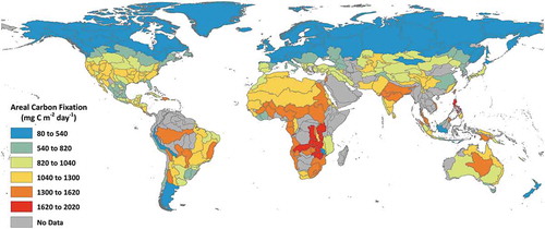
In general, growing season carbon fixation decreases with increasing latitude for both the northern and southern hemispheres. In the southern hemisphere less than < 15% of the freshwater ecoregions had satellite-resolvable lakes whereas in the northern hemisphere about 75% of the ecoregions had satellite-resolvable lakes. Statistically significant regressions were found for carbon fixation and latitude for both hemispheres and there was no significant difference between regression models for northern and southern hemispheres (Figure 4 (a): northern hemisphere, y = −13.5 x + 1279, R² = 0.45, p value < 0.001, N = 217; (b): southern hemisphere, y = −14.8 x + 1227, R² = 0.26, p value < 0.05, N = 16). In the northern hemisphere, latitude alone explained almost 50% of the variation in carbon fixation. Southern hemisphere observations by latitude were more variable than for the northern hemisphere observations; however, fewer observations in the southern hemisphere limit interpretation using FEOW.

Figure 4. Areal carbon fixation (mg C m⁻² day⁻¹) aggregated by freshwater ecoregions of the world vs. latitude for northern (y = −13.479 x + 1279.3, R² = 0.45, p < 0.001, N = 217 and southern hemispheres (y = −14.781 x + 1227.1, R² = 0.26, p = 0.046, N = 16)

Areal carbon fixation also varied significantly by continent (ANOVA p value < 0.001) (Figure 5). Mean fixation rates were significantly different for all continents with the exception of South America and Australia. Africa exhibited the highest mean fixation rates which were about 1.5 times greater than the next highest (South America) and more than four-fold larger than North America and Europe.

Figure 5. Mean continental growing season areal carbon fixation (mg C m⁻² day⁻¹)

When considering all about 80,000 lakes individually, the southern hemisphere generally exhibited carbon fixation rates higher than the northern hemisphere (northern hemisphere: mean = 365, median = 300; southern hemisphere: mean = 1101, median = 1116). This is partially explained by the fact that southern hemisphere lakes are generally located closer to the equator (thus higher ψ values) than the northern hemisphere lakes (southern hemisphere lake latitude: mean = 21.9° S, median 22.5° S; northern hemisphere lake latitude: mean = 60.3° N, median = 62.4° N). However, comparing the mean fixation rates for the southern and northern hemispheres for common latitude ranges (i.e. 0°–30° and 30–60°, no southern lakes further than 60° S) suggested the southern hemisphere exhibits generally higher rates of carbon fixation than the northern hemisphere at similar latitudes. The southern hemisphere mean carbon fixation from 0° to 30° was significantly higher than the northern hemisphere mean fixation rate from 0° to 30° (southern 0° to 30°: mean = 1297; northern 0° to 30°: mean = 968; p value < 0.005). Similarly, the southern hemisphere mean fixation rate for 30–60° was significantly greater than the northern hemisphere fixation rate for the same latitude range (southern 30°–60°: mean = 728; northern 30°–60°: mean = 498; p value < 0.005).

Mean Chl-a concentrations were different between northern and southern hemispheres (northern = 17.6 mg m⁻³; southern = 19.2 mg m⁻³). The biggest differences between hemispheres was for the 0° to 30° latitude range where the northern hemisphere had a mean value of 11.6 mg m⁻³ while the southern hemisphere was 17.1 mg m⁻³. Mean values were similar between the hemispheres for the 30° to 60° latitude range (northern = 18.4 mg m⁻³; southern = 18.5 mg m⁻³).

There was a weak log–log relationship identified between growing season areal carbon fixation rate and lake size for either northern or southern hemispheres (northern hemisphere y = 0.1647 x + 5.448, p value < 0.001, R² = 0.06; southern hemisphere y = 0.0658 x + 6.6793, p value < 0.001, R² = 0.03). Figure 6 is a log-log plot depicting the relationship between lake area and areal carbon fixation for the northern hemisphere (a) and southern hemisphere (b). Even though there is no significant relationship between lake size and fixation rate, general patterns can be perceived. From the plot it can be observed that for both hemispheres lakes larger than 100 km² generally exhibited smaller ranges (about 1 order of magnitude) of areal carbon fixation than did lakes smaller than 100 km² (about 2 orders of magnitude). Similarly, low carbon fixation rates (< 100 mg C m⁻² day⁻¹) are generally observed in lakes smaller than 100 km² in both hemispheres.

Figure 6. Log–log plots of individual lake area and areal carbon fixation for all 80,000 lakes grouped by hemisphere (northern (a), southern (b))

Areal carbon fixation rates aggregated by lake size were compared between northern and southern hemispheres. For each hemisphere, lakes were grouped into size ranges of 0–10, 10–100, 100–1000, > 1000 km². Southern hemisphere mean areal fixation rates were significantly greater than the northern hemisphere mean rates for all lake-size groups (0–10: N = 338, S = 1019, p value < 0.005; 10–100: N = 509, S = 1179, p value < 0.005; 100–1000: N = 630, S = 1194, p value < 0.005; > 1000: N = 594, S = 1279, p value < 0.005). The observed differences in fixation rate by lake size between hemispheres is partially explained by the large number of lakes at far northern latitudes (e.g. > 60° N) and no lakes in the southern hemisphere at the same latitude range. However, comparing mean fixation rates by size groups in the latitude range where lakes are present in both hemispheres (0°–60°) yields similar results to the full latitude comparison. For the common latitude range, southern hemisphere mean areal fixation rates were significantly greater than the northern hemisphere mean rates for all lake-size groups (0–10: N = 480, S = 1019, p value < 0.005; 10–100: N = 665, S = 1179, p value < 0.005; 100–1000: N = 779, S = 1194, p value < 0.005; > 1000: N = 695, S = 1279, p value < 0.005). These results strongly suggest that lakes in the southern hemisphere are more productive than similarly sized lakes in the northern hemisphere.

The DIM approach was also used to estimate the total daily freshwater lake carbon fixation (Tg C day⁻¹) for the global growing season. The total freshwater carbon fixation for the 80,000 lakes was estimated as 1.03 Tg C day⁻¹. The northern hemisphere accounted for about 71% (0.74 Tg C day⁻¹) of the global total while the southern hemisphere accounted for about 29% (0.30 Tg C day⁻¹). The northern hemisphere total fixation was produced from 78,927 lakes (98.6% of all lakes) while the southern hemisphere fixation was produced from just 1074 lakes (1.4% of all lakes). Total freshwater carbon fixation by continent is shown in Figure 7. North America has the highest amount of total fixation (0.52 Tg C day⁻¹) and is almost two-fold larger than Africa (0.28 Tg C day⁻¹). Together North America and Africa account for almost 80% of the global total carbon fixation.

Figure 7. Total continental growing season carbon fixation (Tg C day⁻¹)

A generalized distribution of global freshwater carbon fixation by ecoregion is shown in Figure 8. Approximately 50% of the global carbon fixation is observed in nine ecoregions from North America and Africa (Laurentian Great Lakes, Lake Victoria Basin, English Winnipeg Lakes, Eastern Hudson, Bay Ungava, Southern Hudson Bay, Lake Chad, Western Hudson Bay, Lake Tanganyika, Upper Parana) while more than 25% (about 27%) of the global carbon fixation were from the Laurentian Great Lakes (14.5%) and Lake Victoria Basin (about 13%) alone. Unsurprisingly, very low carbon fixation is observed in the desert regions in Africa and North America. With the exception of the ecoregion areas encapsulating Lake Baikal and Tibetan Plateau, Asia generally has low total carbon fixation. Europe also has generally low total carbon fixation with the exception of Scandinavia.

Figure 8. Total carbon fixation (Tg C day⁻¹) from freshwater lakes aggregated by freshwater ecoregions of the world (Abell et al. 2008)

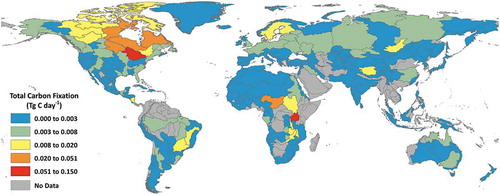
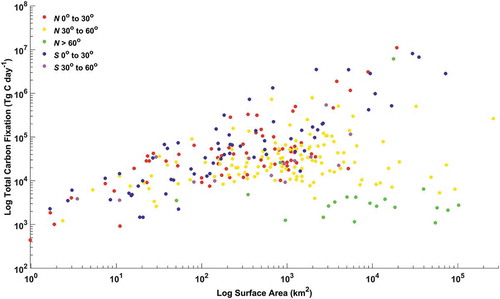
The relationship between total lake surface area and total carbon fixation (areal rate x lake surface area) was assessed by FEOW. A significant correlation between the log₁₀ total surface area and log₁₀ total carbon fixation was identified (Pearson’s correlation coefficient r = 0.37, p value < 0.005). The relationship between total lake surface area and total fixation is shown in Figure 9. Points on the figure are coloured by latitude regions in the northern and southern hemispheres (0°–30° N and S, 30°–60° N and S, > 60° N). Note, there are no lakes in the southern hemisphere beyond 60° S. A general positive trend between total fixation and total surface area is discernible but with high degree of variability. The high latitude lakes in the northern hemisphere are less productive, and appear to be more oligotrophic as they get larger. Ecoregions in the 0°–30° latitude range in both northern and southern hemispheres and the 30°–60° range in the southern follow a similar pattern, while ecoregions in the far northern latitudes deviate from the general trend (e.g. greater lake surface area with lower total carbon fixation in ecoregions > 60° N). Significant differences between the mean total fixation (log₁₀ transformed) of each group were identified (Analysis of variance (ANOVA) p value < 0.005). Ecoregions in the northern hemisphere > 60° N had significantly lower total fixation than all other latitude ranges. All other ecoregion groups were similar with the exception of the southern 0°–30° and northern 30°–60° which were different from each other. The results from these comparisons demonstrate that total freshwater surface area alone is unable to predict total freshwater carbon fixation particularly in high latitudes where areal carbon fixation rates are generally low.

Figure 9. Log–log plots of total lake surface area and total carbon fixation for lakes aggregated by freshwater ecoregions of the world. Data points are coloured by groups (Red: N 0°–30°, Yellow: N 30°–60°, Green: N > 60°, Blue: S 0– 30°, Purple: S 30°–60°)

When considering all about 80,000 lakes individually, significant log–log relationships were identified between lake total carbon fixation and lake size for both northern and southern hemispheres (northern hemisphere y = 1.1647 x + 5.448, p value < 0.001, R² = 0.76; southern hemisphere y = 1.0658 x + 6.6793, p value < 0.001, R² = 0.90). Figure 10 is a log-log plot depicting the relationship between lake area and total carbon fixation for the northern (a) and southern (b) hemispheres. From the figure it can be seen there is a higher degree of variability in total fixation for lakes of smaller size compared to the largest lakes in the northern hemisphere. For example, the coefficient of variation (CoV) for lakes smaller than 1000 km² is about 2.5 fold greater than that for lakes greater than 1000 km² (CoV for > 1000 km² = 2.1; CoV for < 1000 km² = 5.4). Conversely, for the southern hemisphere, similar CoV is observed between lakes greater and smaller than 1000 km² (CoV for > 1000 km² = 2.5; CoV for < 1000 km² = 2.8). Similar to the ecoregion comparison above, these results suggest that estimating global lake carbon fixation based on surface area alone can result in large errors particularly so for smaller lakes which are predominantly located in the far northern latitudes.

Figure 10. Log-log plots of individual lake area and total carbon fixation for all 80,000 lakes grouped by hemisphere (northern (a), southern (b))

4. Discussion and conclusion

The use of remote sensing as a viable tool to estimate carbon fixation from freshwater lakes around the world using a straightforward DIM with an empirically estimated light utilization index has been demonstrated. This method requires very limited input parameters (i.e. Chl-a and irradiance) that are readily available via remote sensing observations. Prior to this study, the use of remote sensing to estimate carbon fixation was limited to application in the marine environment (e.g. Behrenfeld and Falkowski et al. 1997b) and several large freshwater lakes (Lohrenz et al. 2004; Shuchman et al. 2013; Kauer et al. 2015; Warner and Lesht 2015, Fahnenstiel et al. 2016; Deng et al. 2017; Soomets et al. 2019). Carbon fixation remote sensing models vary in form and complexity from highly mechanistic (e.g. Fahnenstiel et al. 2016) to more vertically generalized (e.g. Behrenfeld and Falkowski 1997a) to completely empirical (e.g. Cole and Cloern 1987). Most remote sensing carbon fixation models require a carbon fixation rate parameter (e.g. photosynthesis at light saturation, P_max) or similar value (e.g. quantum yield of carbon fixation) to estimate total carbon fixation, typically from phytoplankton biomass represented as Chl-a concentration or particulate backscatter (e.g. Carbon-based Productivity Model, Behrenfeld et al. 2005; Westberry et al. 2008). The fixation rates are often estimated from water surface temperature (Behrenfeld and Falkowski 1997a, Fahnenstiel et al. 2016; Deng et al. 2017) or chlorophyll concentration (Arst et al. 2012, Soomets et al. 2019) based on empirical relationships derived from in situ data. These established relationships are often broadly used; however, regional tuning often yields more robust results (McClain et al. 2002). The DIM approach utilized here offers a different approach to estimate the carbon fixation parameter (light utilization index) which may offer flexibility in cases where it is not possible to obtain the needed remote sensing input parameters or the empirical models for the other model forms mentioned above are not valid. More importantly the straightforward model we developed to estimate the light utilization index parameter from latitude allows for its broad application to study freshwater production anywhere in the world.

A unique aspect of this project is the first-documented characterization of the light utilization index parameter (ψ) for a variety of freshwater systems throughout the world. The ψ parameter has been relatively well characterized in the marine environment by a variety of investigators (review in Platt 1986) exhibiting an effective range of 0.31–0.66 g C (g Chl)⁻¹ m² (E)⁻¹ while Campbell and O’Reilly (1988) reported a much larger range (about 0.10–10 g C (g Chl)⁻¹ m² (E)⁻¹). The freshwater values reported in this study exhibit a larger range (see Figure 1) than those summarized by Platt (1986) with maximum values more than 1.7 times larger than the marine values but are generally at the lower end of the range reported by Campbell and O’Reilly (1988). The mean freshwater value was similar to the marine value reported by Falkowski (1981) (this study 0.49 vs 0.43) but lower than that of the mean value for the northwest Atlantic continental shelf (1.47 g C (g Chl)⁻¹ m² (E)⁻¹) (Campbell and O’Reilly, 1988). It is expected that ψ values over the entirety of marine and freshwater systems would exhibit similar ranges as phytoplankton in both cases can be exposed to a similar variety of temperature, irradiance, and nutrient conditions resulting in highly variable photosynthetic efficiencies in each environment. Given this variability, it is encouraging that the ψ values for marine and freshwater environments observed in this study are generally similar even with the differences in sampling methods and timing between the many studies considered. The ability to characterize ψ in a variety of environments lends itself as a useful parameter to estimate phytoplankton carbon fixation with limited limnological data sets (e.g. chlorophyll and irradiance).

While this new method for estimating phytoplankton carbon fixation is straightforward to implement and very useful to global studies it is not without limitations. Because the carbon fixation rate is parametrized by latitude spanning the global range (0°–90°) with significant natural variability, it is likely large errors in production could be encountered for any individual lake. In light of these potential errors, this new approach should be implemented when little to know a priori information exists for any given lake system. This limitation, though, does not preclude one from developing their own parametrization of ψ based on any number of predictive variables for their particular system of interest. However, if more complete bio-physical data exists for calibration (e.g. Chl-a concentration, extinction coefficient, temperature, etc), it is expected more sophisticated approaches such as the Great Lakes Production Model (GLPM) (Shuchman et al. 2013; Fahnenstiel et al. 2016) or the Vertically Generalized Production Model (VGPM) (Behrenfeld and Falkowski 1997b) are likely to result in more accurate production estimates.

A surprising observation from this study was that areal carbon fixation rates were not strongly related to lake area. Sayers et al. (2015), using limited comparisons (N = 185) of remote sensing products showed large lakes exhibited lower Chl-a concentrations than medium and small lakes and since primary production is strongly dependent on Chl-a concentrations we thought it would be reasonable to have expected large lakes to exhibit the lowest carbon fixation rate values. However, an extreme number of the smallest lakes are located at far northern latitudes where the light utilization index parameter is lowest resulting in lower carbon fixation rates than previously expected. Moreover, larger lakes tend to be more oligotrophic and thus, have larger photic zones which tend to increase the areal rates. While our observations differed from the limited comparison in Sayers et al. (2015), the results generally agree with those observed by Fee et al. (1992) for a set of variable sized Canadian Shield lakes. The authors noted that areal production for smaller (< 1000 km²) and larger lakes (> 10,000 km²) was generally lower than for medium-sized lakes (1000 to 10,000 km²) due to in part to increased Chl-a biomass and not differing photosynthetic parameters. It is hypothesized that medium-sized lakes generally exhibit higher areal production due to the combined offset of two parameters (temperature and turbulence) supporting increased phytoplankton growth. Our results do indicate that the smallest lakes have the lowest production rates; however, we also observe very high rates in smaller lakes in both hemispheres. It is difficult to compare production rates by lake size over the full latitude range as the light utilization parameter also strongly influences production rates. The combined effects of variable Chl-a concentration, light utilization rate, and irradiance across continents and hemispheres underscores the complexity of estimating lake production over large scales. Future work is needed to better understand the lake-size effect on carbon fixation rates for regions of similar photosynthetic efficiencies (i.e. similar latitude in our model).

The new remote sensing method reported here offers new insights into regional and local carbon fixation patterns that cannot be resolved with model based approaches. Historically, carbon fixation from global freshwater lakes has been estimated using model based approaches that assume the global total number of lakes and their size distribution. For example, Lewis (2011) utilized a Monte Carlo simulation based approach to estimate global freshwater lake production accounting for deterministic and stochastic controlling factors and latitudinal models of lake size and abundance distributions. And while this approach is very useful for generating a total global freshwater production estimate for comparison with terrestrial and marine production, it lacks the ability to provide spatial information at regional and local scales throughout the world. Our new remote sensing based approach provides this granularity based on actual observations of individual lakes thus providing estimates that are more robust for any particular region in the world. This is a critical capability that is needed to understand how local factors control rates of production in lakes.

Application of the new DIM approach resulted in an improved understanding of global spatial variation of areal and total carbon fixation rates. Prior to this work, spatial comparisons of freshwater fixation rates have been made using spatially limited in situ measurements, often utilizing different techniques, making it difficult to draw quantitative conclusions (Fahnenstiel et al. 2016). Results from this study indicated that southern hemisphere lakes, particularly those in Africa, are generally more productive than lakes in the northern hemisphere for similar latitude ranges. We hypothesize the elevated production in southern hemisphere lakes is attributable to the increased nutrient levels likely due to human activity. This is supported for tropical latitude ranges (0°–30°) where the southern hemisphere mean Chl-a concentration was almost 50% larger than that of the northern hemisphere. Lakes in the southern hemisphere are generally more accessible than lakes in the northern hemisphere naturally inviting more human interaction thus generally increasing the availability of nutrients stimulating phytoplankton growth. Conversely, lakes in the northern hemisphere are highly concentrated in extreme northern latitudes that were previously glaciated (Raymond et al. 2013). The sheer remoteness of these lakes limits the impact from humans resulting in limited nutrient availability primarily controlled by the surrounding natural landscape (i.e. rock). Even northern hemisphere lakes at more moderate latitudes (< 45° N) are less inviting to human activity as they are generally located in more mountainous areas particularly in southern Asia and mid-North America.

Knowing how much and where freshwater carbon fixation occurs is critical for improved understanding of Earth’s carbon budget. Even though freshwater lakes account for only 4% of the surface of the Earth (Verpoorter et al. 2014) they are a significant contributor to the overall carbon cycle (Tranvik et al. 2009) thus underlying the importance of their accurate characterization. Freshwater carbon cycling models rely on parameterizations of the different modes CO₂ is transported through a lake system. These parameterizations are critical for producing accurate estimates of carbon flux and ultimately determine whether a given lake is a carbon sink or a carbon source (Engel et al. 2018). The new carbon fixation data set produced in this study can fill a gap in these parameterizations that have previously assumed ‘all lakes on Earth function similarly’ (Engel et al. 2018). With improved estimates of photosynthetic rates for many lakes in the world, modellers can begin to realize the magnitude of the effect lake composition has on flux calculations. Moreover, the spatial context of the new remote sensing freshwater products provides the opportunity to study regional carbon cycling dynamics that were previously lacking a key component (i.e. lake carbon fixation). Assessing these effects over time may also shed light into what the future may look like in the face of climate change and anthropogenic forcing (Engel et al. 2018).

In conclusion, this work resulted in the first remote sensing derived estimates of global freshwater lake phytoplankton carbon fixation which represents a crucial first step towards fully understanding global lake carbon budgets. The straightforward DIM presented here is valuable tool to estimate freshwater phytoplankton production anywhere in the world with only minimal remote sensing or field-measured data. Because of this flexibility, the new model is well suited for adaptation to airborne and unmanned aerial systems (UAS) to potentially estimate phytoplankton carbon fixation in small systems too small to be observed from space including ponds and rivers. Moreover, the extensible nature of this approach allows for a truly global analysis of carbon fixation rates which can be assessed relative to regional and local scale anthropogenic forcing, which is not possible with current model-based approaches. Additionally, future implementation of the DIM approach to more robust remote sensing based time-series observations, including observations in far more than 80,000 lakes, will likely provide valuable and descriptive insights into the role climate change has on regional and global carbon cycle dynamics.

Data Availability

Upon publication, the data presented in this manuscript will be available from the NASA Carbon Monitoring System (https://carbon.nasa.gov/cgi-bin/cms_projects.pl#current2016)

Acknowledgements

The authors express their appreciation to Katherine Laramie and Zane Almquist for assistance with literature search and data processing. The authors also wish thank an anonymous reviewer for their thoughtful comments that resulted in an improved manuscript. Any use of trade, product, or firm names is for descriptive purposes only and does not imply endorsement by the US Government

Disclosure statement

No potential conflict of interest was reported by the authors.

Additional information

Funding

This work was supported by The National Aeronautics and Space Administration (NASA) Carbon Monitoring System [contract number: 80NSSC17K0712].

References

- Abell, R., M. L. Thieme, C. Revenga, M. Bryer, M. Kottelat, N. Bogutskaya, B. Coad, et al. 2008. “Freshwater Ecoregions of the World: A New Map of Biogeographic Units for Freshwater Biodiversity Conservation.” BioScience 58 (5): 403–414. doi:10.1641/B580507.
- Amarasinghe, P. B., and J. Vijverberg. 2002. “Primary Production in a Tropical Reservoir in Sri Lanka.” Hydrobiologia 487 (1): 85–93. doi:10.1023/A:1022985908451.
- Arst, H., Nõges, P., Nõges, T. et al. Quantification of a Primary Production Model Using Two Versions of the Spectral Distribution of the Phytoplankton Absorption Coefficient. Environ Model Assess 17, 431–440 (2012). https://doi.org/10.1007/s10666-011-9305–z
- Behrenfeld, M., and P. Falkowski. 1997a. “A Consumer’s Guide to Phytoplankton Primary Productivity Models.” Limnology and Oceanography 42: 1479–1491. doi:10.4319/lo.1997.42.7.1479.
- Behrenfeld, M. J., E. Boss, D. A. Siegel, and D. M. Shea. 2005. “Carbon‐based Ocean Productivity and Phytoplankton Physiology from Space.” Global Biogeochemical Cycles 19 (1). doi:10.1029/2004GB002299.
- Behrenfeld, M. J., and P. G. Falkowski. 1997b. “Photosynthetic Rates Derived from Satellite‐based Chlorophyll Concentration.” Limnology and Oceanography 42 (1): 1–20. doi:10.4319/lo.1997.42.1.0001.
- Bennington, V., G. A. McKinley, N. R. Urban, and C. P. McDonald. 2012. “Can Spatial Heterogeneity Explain the Perceived Imbalance in Lake Superior’s Carbon Budget? A Model Study.” Journal of Geophysical Research 117: G03020.
- Bergmann, T., G. Fahnenstiel, S. Lohrenz, D. Millie, and O. Schofield. 2004. “The Impacts of a Recurrent Resuspension Event and Variable Phytoplankton Community Composition on Remote Sensing Reflectance.” Journal of Geophysical Research 109: C10S15.
- Berman, T., L. Stone, Y. Z. Yacobi, B. Kaplan, A. Schlichter, A. Nishri, and U. Pollingher. 1995. “Primary Production and Phytoplankton in Lake Kinneret: A Long‐term Record (1972‐1993).” Limnology and Oceanography 40 (6): 1064–1076. doi:10.4319/lo.1995.40.6.1064.
- Binding, C. E., T. A. Greenberg, and R. P. Bukata. 2012. “An Analysis of MODIS-derived Algal and Mineral Turbidity in Lake Erie.” Journal of Great Lakes Research 38 (1): 107–116. doi:10.1016/j.jglr.2011.12.003.
- Bindloss, M. E., 1974. Primary Productivity of Phytoplankton in Loch Leven, Kinross. Proceedings of the Royal Society of Edinburgh, Section B: Biological Sciences, 74, 157–181.
- Bricaud, A., M. Babin, A. Morel, and H. Claustre. 1995. “Variability in the Chlorophyll‐specific Absorption Coefficients of Natural Phytoplankton: Analysis and Parameterization.” Journal of Geophysical Research: Oceans 100 (C7): 13321–13332. doi:10.1029/95JC00463.
- Buffam, I., M. G. Turner, A. Desaiz, P. C. Hanson, J. A. Rusak, N. R. Lottig, E. H. Stanley, and S. R. Carpenter. 2011. “Integrating Aquatic and Terrestrial Components to Construct a Complete Carbon Budget for a North Temperate Lake District.” Global Change Biology 17 (2): 1193–1211. doi:10.1111/j.1365-2486.2010.02313.x.
- Bukata, R., J. Jerome, K. Kondratyev, and D. Pozdnyakov. 1995. Optical Properties of Inland and Coastal Waters. Florida, Boca Raton.CRC Press
- Campbell, Janet W., and O'Reilly, John E. “Role of satellites in estimating primary productivity on the northwest Atlantic continental shelf.„ Continental Shelf Research 8, no. 2 (1988): 179–204
- Cole, B. E., and J. E. Cloern. 1987. “An Empirical Model for Estimating Phytoplankton Productivity in Estuaries.” Marine Ecology Progress Series 36 (1): 299–305. doi:10.3354/meps036299.
- Cole, J. J., Y. T. Prairie, N. F. Caraco, W. H. McDowell, L. J. Tranvik, R. G. Striegl, C. M. Duarte, et al. 2007. “Plumbing the Global Carbon Cycle: Integrating Inland Waters into the Terrestrial Carbon Budget.” Ecosystems 10: 171–184. doi:10.1007/s10021-006-9013-8.
- Darchambeau, F., H. Sarmento, and J. P. Descy. 2014. “Primary Production in a Tropical Large Lake: The Role of Phytoplankton Composition.” Science of the Total Environment 473: 178–188. doi:10.1016/j.scitotenv.2013.12.036.
- Deng, Y., Y. Zhang, D. Li, K. Shi, and Y. Zhang. 2017. “Temporal and Spatial Dynamics of Phytoplankton Primary Production in Lake Taihu Derived from MODIS Data.” Remote Sensing 9 (3): 195.
- Dobson, H. F., M. Gilbertson, and P. G. Sly. 1974. “A Summary and Comparison of Nutrients and Related Water Quality in Lakes Erie, Ontario, Huron, and Superior.” Journal of the Fisheries Board of Canada 31 (5): 731–738. doi:10.1139/f74-099.
- Dokulil, M., I. Silva, and K. Bauer. 1983. “An Assessment of the Phytoplankton Biomass and Primary Productivity of Parakrama Samudra, a Shallow Man-made Lake in Sri Lanka.” In Limnology of Parakrama Samudra—Sri Lanka, edited by Schiemer, F., 49–76. Dr W. Junk Publishers, The Hague.
- Edmondson, W. T. 1979. “Lake Washington and the Predictability of Limnological Events.” Ergebnisse der Limnologie 13: 234–241.
- Engel, F., K. J. Farrell, I. M. McCullough, F. Scordo, B. A. Denfeld, H. A. Dugan, E. de Eyto, et al. 2018. “A Lake Classification Concept for A More Accurate Global Estimate of the Dissolved Inorganic Carbon Export from Terrestrial Ecosystems to Inland Waters.” The Science of Nature 105 (3–4): 25. doi:10.1007/s00114-018-1547-z.
- Fahnenstiel, G., M. J. Sayers, R. A. Shuchman, F. Yousef, and S. A. Pothoven. 2016. “Lake-wide Phytoplankton Production and Abundance in the Upper Great Lakes: 2010–2013.” Journal of Great Lakes Research 42 (3): 619–629. doi:10.1016/j.jglr.2016.02.004..
- Falkowski, P. G. 1981. “Light-shade Adaptation and Assimilation Numbers.” Journal of Plankton Research 3 (2): 203–216. doi:10.1093/plankt/3.2.203.
- Fee, E. J., J. A. Shearer, E. R. DeBruyn, and E. V. Schindler. 1992. “Effects of Lake Size on Phytoplankton Photosynthesis.” Canadian Journal of Fisheries and Aquatic Sciences 49 (12): 2445–2459. doi:10.1139/f92-270.
- Gelin, C., 1971. Primary Production and Chlorophyll a Content of Nanoplankton in a Eutrophic Lake. Oikos, 230–234.
- Gilerson, A., J. Zhou, S. Hlaing, I. Ioannou, J. Schalles, B. Gross, F. Moshary, and S. Ahmed. 2007. “Fluorescence Component in the Reflectance Spectra from Coastal Waters. Dependence on Water Composition.” Optics Express 15 (24): 15702–15721. doi:10.1364/OE.15.015702.
- Goldman, C. R. 1977. Trophic Status and Nutrient Loading for Lake Tahoe, 465. North American Project: A Study of US Water Bodies.
- Gons, H. J., M. T. Auer, and S. W. Effler. 2008. “MERIS Satellite Chlorophyll Mapping of Oligotrophic and Eutrophic Waters in the Laurentian Great Lakes.” Remote Sensing of Environment 112: 4098–4106. doi:10.1016/j.rse.2007.06.029.
- Guildford, S. J., H. A. Bootsma, W. D. Taylor, and R. E. Hecky. 2007. “High Variability of Phytoplankton Photosynthesis in Response to Environmental Forcing in Oligotrophic Lake Malawi/Nyasa.” Journal of Great Lakes Research 33 (1): 170–185. doi:10.3394/0380-1330(2007)33[170:HVOPPI]2.0.CO;2.
- Hecky, R. E., and E. J. Fee. 1981. “Primary production and rates of algal growth in Lake Tanganyika.„ Limnology and Oceanography 26(3): 532–547.
- Hecky, R. E., E. J. Fee, H. Kling, and J. W. M. Rudd. 1978. Studies on the Planktonic Ecology of Lake Tanganyika. Winnipeg, Man: Fisheries and Marine Service.
- Hunter, P. D., A. N. Tyler, L. Carvalho, G. A. Codd, and S. C. Maberly. 2010. “Hyperspectral Remote Sensing of Cyanobacterial Pigments as Indicators for Cell Populations and Toxins in Eutrophic Lake.” Remote Sensing Environment 114: 2705–2718. doi:10.1016/j.rse.2010.06.006.
- Kalff, J., and H. E. Welch. 1974. “Phytoplankton Production in Char Lake, a Natural Polar Lake, and in Meretta Lake, a Polluted Polar Lake, Cornwallis Island, Northwest Territories.” Journal of the Fisheries Board of Canada 31 (5): 621–636. doi:10.1139/f74-094.
- Kauer, T., T. Kutser, H. Arst, T. Danckaert, and T. Nõges. 2015. “Modelling Primary Production in Shallow Well Mixed Lakes Based on MERIS Satellite Data.” Remote Sensing of Environment 163: 253–261. doi:10.1016/j.rse.2015.03.023.
- Kerekes, J. 1974. “Limnological Conditions in Five Small Oligotrophic Lakes in Terra Nova National Park, Newfoundland.” Journal of the Fisheries Board of Canada 31 (5): 555–583. doi:10.1139/f74-091.
- Kerekes, J. 1975. “Phosphorus Supply in Undisturbed Lakes in Kejimkujik National Park, Nova Scotia (Canada) with 4 Figures and 2 Tables in the Text.” Internationale Vereinigung für theoretische und angewandte Limnologie: Verhandlungen 19 (1): 349–357.
- Larsen, S., T. Anderson, and D. O. Hessen. 2011. “Climate Change Predicted to Cause Severe Increase in Organic Carbon in Lakes.” Global Change Biology 17: 1186–1192. doi:10.1111/j.1365-2486.2010.02257.x.
- Lee, Z. 2005. “A Model for the Diffuse Attenuation Coefficient of Downwelling Irradiance.” Journal of Geophysical Research 110 (C2). doi:10.1029/2004jc002275.
- Lee, Z., A. Weidemann, J. Kindle, R. Arnone, K. L. Carder, and C. Davis. 2007. “Euphotic Zone Depth: Its Derivation and Implication to Ocean-color Remote Sensing.” Journal of Geophysical Research 112 (C3). doi:10.1029/2006jc003802.
- Lemoalle, J. 1981. “Photosynthetic Production and Phytoplankton in the Euphotic Zone of Some African and Temperate Lakes.” Revue d’Hydrobiologie tropicale 14 (1): 31–37.
- Lewis Jr, W. M. 2011. “Global Primary Production of Lakes: 19th Baldi Memorial Lecture.” Inland Waters 1 (1): 1–28. doi:10.5268/IW-1.1.384.
- Lohila, A., J. Tuovinen, J. Hatakka, M. Aurela, J. Vuorenmaa, M. Haakana, and T. Laurila. 2015. “Carbon Dioxide and Energy Fluxes over a Northern Boreal Lake.” Boreal Environment Research 20: 474–488.
- Lohrenz, S. E., G. L. Fahnenstiel, D. F. Millie, O. M. E. Schofield, T. Johengen, and T. Bergman. 2004. “Spring Phytoplankton Photosynthesis, Growth, and Primary Production and Relationships to a Recurrent Coastal Sediment Plume and River Inputs in Southeastern Lake Michigan.” Journal of Geophysical Research 109 (C10): C10S14.
- Lohrenz, S. E., G. L. Fahnenstiel, O. M. E. Schofield, and D. F. Millie. 2008. “Coastal Sediment Dynamics and River Discharge as Key Factors Influencing Coastal Ecosystem Productivity in Southeastern Lake Michigan.” Oceanography 21: 54–63. doi:10.5670/oceanog.2008.05.
- Marzolf, G. R., and J. A. Osborne. 1972. “Primary Production in a Great Plains Reservoir.” Internationale Vereinigung für theoretische und angewandte Limnologie: Verhandlungen 18 (1): 126–133.
- McClain, C.R., Christian, J.R., Signorini, S.R., Lewis, M.R., Asanuma, I., Turk, D. and Dupouy-Douchement, C., 2002. Satellite ocean-color observations of the tropical Pacific Ocean. Deep Sea Research Part II: Topical Studies in Oceanography, 49(13–14), pp.2533–2560
- McCree, K. J. 1981. “Photosynthetically Active Radiation.” O. L. Lange et al.(eds.), In Physiological Plant Ecology I, 41–55. Berlin, Springer-Verlag Berlin · Heidelberg 1981.
- Megard, R. O. 1972. “Phytoplankton, Photosynthesis, and Phosphorus in Lake Minnetonka, Minnesota 1.” Limnology and Oceanography 17 (1): 68–87. doi:10.4319/lo.1972.17.1.0068.
- Megard, R. O., and P. D. Smith. 1974. “Mechanisms that Regulate Growth Rates of Phytoplankton in Shagawa Lake, Minnesota 1.” Limnology and Oceanography 19 (2): 279–296. doi:10.4319/lo.1974.19.2.0279.
- Melack, J. M. 1979. “Photosynthetic Rates in Four Tropical African Fresh Waters.” Freshwater Biology 9 (6): 555–571. doi:10.1111/j.1365-2427.1979.tb01539.x.
- Michalski, M. F. P., M. G. Johnson, D. M. Veal, and T. G. Brydges, 1973. Muskoka Lakes Water Quality Evaluation. Ministry of the Environment.
- Millard, E. S., D. D. Myles, O. E. Johannsson, and K. M. Ralph. 1996. “Phytoplankton Photosynthesis at Two Index Stations in Lake Ontario 1987-1992: Assessment of the Long-term Response to Phosphorus Control.” Canadian Journal of Fisheries and Aquatic Sciences 53 (5): 1092–1111.
- Moss, D., S. Kosten, M. Meerhoff, R. W. Battarbee, E. Jeppeson, N. Mazzeo, K. Havens, et al. 2011. “Allied Attack: Climate Change and Eutrophication.” Inland Waters 1: 101–105. doi:10.5268/IW-1.2.359.
- O’Reilly, J. E., S. Maritorena, B. G. Mitchell, D. A. Siegel, K. L. Carder, S. A. Garver, M. Kahru, and C. McClain. 1998. “Ocean Color Chlorophyll Algorithms for SeaWiFS.” Journal of Geophysical Research: Oceans 103 (C11): 24937–24953. doi:10.1029/98JC02160.
- Patterson, G., R. E. Hecky, and E. J. Fee. 2000. “Effect of Hydrological Cycles on Planktonic Primary Production in Lake Malawi/Niassa.” Advances in Ecological Research 31: 421–430.
- Platt, T. 1986. “Primary Production of the Ocean Water Column as A Function of Surface Light Intensity: Algorithms for Remote Sensing. Deep Sea Research Part A.” Oceanographic Research Papers 33 (2): 149–163. doi:10.1016/0198-0149(86)90115-9.
- Pope, R. M., and E. S. Fry. 1997. “Absorption Spectrum (380–700 Nm) of Pure Water. II. Integrating Cavity Measurements.” Applied Optics 36 (33): 8710–8723. doi:10.1364/AO.36.008710.
- Porta, D., M. A. Fitzpatrick, and G. D. Haffner. 2005. “Annual Variability of Phytoplankton Primary Production in the Western Basin of Lake Erie (2002–2003).” Journal of Great Lakes Research 31: 63–71. doi:10.1016/S0380-1330(05)70305-1.
- Raymond, P. A., J. Hartmann, R. Lauerwald, S. Sobek, C. McDonald, M. Hoover, D. Butman, et al. 2013. “Global Carbon Dioxide Emissions from Inland Waters.” Nature 503 (7476): 355. doi:10.1038/nature12760.
- Regnier, P., P. Friedlingstein, P. Ciais, F. T. Mackenzie, N. Gruber, I. A. Janssens, … S. Arndt. 2013. “Anthropogenic Perturbation of the Carbon Fluxes from Land to Ocean.” Nature Geoscience 6 (8): 597–607. doi:10.1038/ngeo1830.
- Rousar, D. C. 1973. “Seasonal and Spatial Changes in Primary Production and Nutrients in Lake Michigan.” Water, Air, and Soil Pollution 2 (4): 497–514. doi:10.1007/BF00585093.
- Saha, S., S. Moorthi, X. Wu, J. Wang, S. Nadiga, P. Tripp, D. Behringer, et al. 2014. “The NCEP Climate Forecast System Version 2.” Journal of Climate 27 (6): 2185–2208. doi:10.1175/JCLI-D-12-00823.1.
- Saulquin, B., A. Hamdi, F. Gohin, J. Populus, A. Mangin, and O. F. d’Andon. 2013. “Estimation of the Diffuse Attenuation Coefficient KdPAR Using MERIS and Application to Seabed Habitat Mapping.” Remote Sensing of Environment 128: 224–233. doi:10.1016/j.rse.2012.10.002.
- Sayers, M. J., A. G. Grimm, R. A. Shuchman, A. M. Deines, D. B. Bunnell, Z. B. Raymer, M. W. Rogers, et al. 2015. “A New Method to Generate A High Resolution Global Distribution Map of Lake Chlorophyll.” International Journal of Remote Sensing 36: 1942–1964. doi:10.1080/01431161.2015.1029099.
- Schindler, D. W. 1972. “The Dependence of Primary Production upon Physical and Chemical Factors in a Small, Senescing Lake, Including the Effects of Complete Winter Oxygen Depletion.” Archiv Fur Hydrobiologie 69: 413–451.
- Shuchman, R., M. Sayers, C. Brooks, G. Fahnenstiel, and G. Leshkevich. 2013. “A Model for Determining Satellite- Derived Primary Productivity Estimates for Lake Michigan.” Journal of Great Lakes Research 39 (S1): 46–54. doi:10.1016/j.jglr.2013.05.001.
- Soomets, T., T. Kutser, A. Wüest, and D. Bouffard. 2019. “Spatial and Temporal Changes of Primary Production in a Deep Peri-alpine Lake.” Inland Waters 9 (1): 49–60. doi:10.1080/20442041.2018.1530529.
- Stenuite, S., S. Pirlot, M. A. HARDY, H. Sarmento, A. L. TARBE, B. Leporcq, and J. P. DESCY. 2007. “Phytoplankton Production and Growth Rate in Lake Tanganyika: Evidence of a Decline in Primary Productivity in Recent Decades.” Freshwater Biology 52 (11): 2226–2239. doi:10.1111/j.1365-2427.2007.01829.x.
- Tilahun, G., and G. Ahlgren. 2010. “Seasonal Variations in Phytoplankton Biomass and Primary Production in the Ethiopian Rift Valley Lakes Ziway, Awassa and Chamo–The Basis for Fish Production.” Limnologica-Ecology and Management of Inland Waters 40 (4): 330–342. doi:10.1016/j.limno.2009.10.005.
- Tranvik, L. J., J. A. Downing, J. B. Cotner, S. A. Loiselle, R. G. Striegl, T. J. Ballatore, … P. L. Dillon. 2009. “Lakes and Reservoirs as Regulators of Carbon Cycling and Climate.” Limnology and Oceanography 54 (6part2): 2298–2314. doi:10.4319/lo.2009.54.6_part_2.2298.
- Verpoorter, C., T. Kutser, D. A. Seekell, and L. J. Tranvik. 2014. “A Global Inventory of Lakes Based on High‐resolution Satellite Imagery.” Geophysical Research Letters 41 (18): 6396–6402. doi:10.1002/2014GL060641.
- Vollenweider, R. A., M. Munawar, and P. Stadelmann. 1974. “A Comparative Review of Phytoplankton and Primary Production in the Laurentian Great Lakes.” Journal of the Fisheries Research Board of Canada 31 (5): 739–762. doi:10.1139/f74-100.
- Warner, D. M., and B. M. Lesht. 2015. “Relative Importance of Phosphorus, Invasive Mussels and Climate for Patterns in Chlorophyll a and Primary Production in Lakes Michigan and Huron.” Freshwater Biology 60 (5): 1029–1043. doi:10.1111/fwb.12569.
- Weiss, C. M., and H. Noore. 1977. The John H. Kerr Reservoir, 426. Virginia- North Carolina: NATIONAL TECHNICAL lNFORMATlQN SERVICE.
- Welch, E. B., T. Wiederholm, D. E. Spyridakis, and C. A. Rock. 1977. Nutrient Loading and Trophic State of Lake Sammamish. Washington: North American Project–A Study of U. S. Water Bodies.
- Westberry, T., M. J. Behrenfeld, D. A. Siegel, and E. Boss. 2008. “Carbon‐based Primary Productivity Modeling with Vertically Resolved Photoacclimation.” Global Biogeochemical Cycles 22 (2). doi:10.1029/2007GB003078.
- Whalen, S. C., B. A. Chalfant, E. N. Fischer, K. A. Fortino, and A. E. Hershey. 2006. “Comparative Influence of Resuspended Glacial Sediment on Physicochemical Characteristics and Primary Production in Two Arctic Lakes.” Aquatic Sciences 68 (1): 65–77. doi:10.1007/s00027-005-0804-3.
- Williamson, C. E., J. E. Saros, W. F. Vincent, and J. P. Smol. 2009. “Lakes and Reservoirs as Sentinels, Integrators, and Regulators of Climate Change.” Limnology and Oceanography 54: 2273–2282. doi:10.4319/lo.2009.54.6_part_2.2273.
- Winner, R. W. 1972. “An Evaluation of Certain Indices of Eutrophy and Maturity in Lakes.” Hydrobiologia 40 (2): 223–245. doi:10.1007/BF00016795.
- Wright, J. C. 1959. “Limnology of Canyon Ferry Reservoir: II. Phytoplankton Standing Crop and Primary Production.” Limnology and Oceanography 4 (3): 235–245. doi:10.4319/lo.1959.4.3.0235.