Data fusion approach for eucalyptus trees identification

ABSTRACT

Remote sensing is based on the extraction of data, acquired by satellites or aircrafts, through multispectral images, that allow their remote analysis and classification. Analysing those images with data fusion techniques is a promising approach for identification and classification of forest types. Fusion techniques can aggregate various sources of heterogeneous information to generate value-added maps, facilitating forest-type classification. This work applies a data fusion algorithm, denoted FIF (Fuzzy Information Fusion), which combines computational intelligence techniques with multicriteria concepts and techniques, to automatically distinguish Eucalyptus trees from satellite images. The algorithm customization was performed with a Portuguese area planted with Eucalyptus. After customizing and validating the approach with several representative scenarios to assess its suitability for automatic classification of Eucalyptus, we tested on a large tile obtaining a sensitivity of 69.61%, with a specificity of 99.43%, and an overall accuracy of 98.19%. This work demonstrates the potential of our approach to automatically classify specific forest types from satellite images, since this is a novel approach dedicated to the identification of eucalyptus trees.

1. Introduction

The identification/classification of land types can be a cumbersome task (e.g. forests, water bodies, and cultivation fields) and has become a very important topic in recent years, particularly to support public entities in the monitorization and management of different land types (Desclée, Bogaert, and Defourny 2006).

Direcção Geral do Território (DGT) is a Portuguese public entity working on the identification and classification of the Portuguese territory, providing a cartography map, denoted Soil Occupation Charts (SOC), which divides the country map into polygons of different types of land. Although this service is very useful, it has two main problems. First, it is a manual process; hence, it takes a long time to execute. Second, due to low image resolution and diversity of land (e.g. forests, roads, houses), it is a difficult and relatively imprecise process to classify their classes; hence, they simplify the process by using a minimum cartographic unit of 1 ha and a minimum distance between lines of 20 m. Due to these properties, it is possible to observe, for example, dirt-roads crossing areas identified with Eucalyptus or examples where different types of trees are mixed in the 1 ha area (e.g. pine trees), but are still classified as Eucalyptus. Therefore, it is of paramount importance to improve the automatic classification of land types to enable better monitoring of unlawful landscape changes or supporting precision agriculture (Taylor, Brewer, and Bird 2000; Antrop 2004) and improve the inventory, assessment and monitoring of other types of lands (Davidson and Finlayson 2007).

2. Objectives

Satellite image classification goes through several processes (Gallego and Stibig 2013; Ribeiro et al. 2014; Lavreniuk et al. 2016) and starts by capturing soil properties (physical and chemical) from satellites (digital images) (Baumgardner et al. 1986; Ben-Dor, Inbar, and Chen 1997; Sumfleth and Duttmann 2008) to enable the analysis of images in order to identify different land types using tailored algorithms.

Having the above in mind, the objectives of this work are to adapt an existing tool, Fuzzy Information Fusion (FIF) algorithm (Ribeiro et al. 2014), to automatically identify a specific type of tree (Eucalyptus), demonstrating the versatility and efficacy of that tool for forestry classification.

This work focuses on eucalyptus because its plantation area is increasing in Portugal and other paper-producing countries. Eucalyptus was chosen because of the following relevant characteristics: being a fast-growing tree it provides a quick return on investment; they are the main supplier of raw material for cellulose industries; being an environmental damaging tree (e.g. nutrients consumption) it requires monitoring of changes in unlawful landscape (Garcia 2017). According to the 6th Portuguese Forest Inventory (ICNF 2019), forests occupy near 35% of the total Portuguese soil and around 23% of them are occupied by eucalyptus. This is a national problem because planting new eucalyptus might not be a good option in the long term, due to their high water consumption and high flammability, which causes a large interference on neighbouring vegetation species (Liu and Li 2010). This study contributes to the implementation of an automatic Eucalyptus tree identification tool, as most of the previous work is based on manual classification, with a few studies using data fusion algorithms (Ali, Dare, and Jones 2008; Haywood and Stone 2011).

3. Related work

3.1. Computational intelligence approaches

Recently, several Computational Intelligent (CI) approaches for data fusion were proposed, for usage in remote sensing approaches (Fauvel, Chanussot, and Benediktsson 2006; Ayhan and Kansu 2012). Examples of those techniques are Decision Trees (DT), Artificial Neural Networks (ANN), or Fuzzy Inference Systems (FIS) (Friedl and Brodley 1997; Kanellopoulos and Wilkinson 1997; Fauvel, Chanussot, and Benediktsson 2006; Ross 2004).

Decision Trees – Well-known classification method that consists of splitting input data into smaller subsets with similar features. DT are composed of nodes and leaves, where each node represents a rule applied to the data. The most commonly used evaluation algorithms are ID3, C4.5 or CART; they have been applied in remote sensing land classification since the 90s (Friedl and Brodley 1997; Xu et al. 2005; Fauvel, Chanussot, and Benediktsson 2006; Colditz 2015; A. Mora et al. 2017; A. D.2016), with a particular approach used for eucalyptus identification (Piiroinen et al. 2017).

Artificial Neural Networks – Classification technique based on a cluster of neurons where each connection transmits signals from one neuron to another. ANN can be multi-layer, where the number of artificial neurons in the input and output is determined by the data being analysed, whereas the number of hidden layers is normally defined by trial and error (Ayhan and Kansu 2012). Examples of land cover classification with ANN can be seen in (A. Mora et al. 2017; A. D.2016; Graciela Canziani Claudia Marinelli, Federico Dukatz 2008; Mas and Flores 2008; Yang et al. 2018).

Fuzzy Inference Systems – This technique has been the basis for data fusion procedures (Ribeiro et al. 2014). FIS are based on rules, defined by logic operators, where the rules establish relationships between fuzzy sets (input variables). It has been tested in several land cover problems (Reshmidevi, Eldho, and Jana 2009; Jenicka 2018).

Further, with the objective of discussing the suitability of different computational intelligence methods for studying land cover spatiotemporal modifications, this FIS algorithm (Ribeiro et al. 2014) was compared with Decision Trees and ANN methods, for fusing images (A. D. Mora et al. 2015; A. D.2016; A.2017), with these studies fusing spectral information to produce land cover maps. However, those studies only classified general classes, such as vegetation and water bodies, not distinguishing between different types of forest trees.

In summary, CI techniques applied to data fusion are proving to be useful tools for the classification of land types in remote sensing (Schmitt and Zhu 2016; Chang and Bai 2018; Ghamisi et al. 2019).

3.2. Data fusion approaches

Data fusion consists of a process of aggregating data from various sources to construct a single compound with higher quality of information (Hyder, Shahbazian, and Waltz 2012; Bleiholder and Naumann 2009; Lee et al. 2010). It includes three main types: image fusion, multisensor fusion, and information fusion (Hyder, Shahbazian, and Waltz 2012), where the common factor is that all sources must focus on the same subject/area:

Image fusion – The main objective of image fusion is to decrease uncertainty and redundancy, thus maximizing pertinent information by merging several image representations of the same scene (Ardeshir Goshtasby and Nikolov 2007). Algorithms of this sort are usually divided into two groups: pixel-based and feature-based (Dai and Khorram 1999). In the first one, the most common, data are fusing pixel-by-pixel, while in the second one, fusion requires extraction and fusion of features from different sources (Piella 2003; Hsu et al. 2009).

Multisensor fusion – This method refers to the fusion of data provided by sensors and its main goal is to assimilate data measurements, extracted from different sensors, and combine them into a single representation (Ribeiro et al. 2014). Some approaches use statistical methods (Kalman filter) and/or probabilistic techniques (Bayesian networks) and others use hybrid models (Klein 2004; Zhang and Xiaolin 2006; Paliwal and Kumar 2009; Lee et al. 2010).

Information fusion – Information fusion is a multi-level process of combining different data to produce fused information (Torra and Narukawa 2007; Lee et al. 2010). There is a tenuous line between image fusion and information fusion because feature and symbolic levels of fusion can be considered image fusion, but they can also be considered as information-based fusion (Piella 2003). This type of data fusion can be defined as a multilevel process of integrating information from multi-sources to produce fused information (Lee et al. 2010).

Data fusion approaches, based on fuzzy logic techniques, are emerging as a technique for land classification to perform correct reasoning inferences (Hyder, Shahbazian, and Waltz 2012; Santos, Andre Mora, and Joao 2016). The FIF algorithm – basis of our approach – is based on fuzzy logic and specialized decision-making aggregation operators and was applied to spacecraft landing with hazard avoidance (Bourdarias et al. 2010; Câmara et al. 2015) as well as for land cover classification (A. D. Mora et al. 2015; A. D.2016; A.2017).

3.3. Eucalyptus tree identification

Eucalyptus trees have unique characteristics, as for instance, their height and their biomass content (Le Maire et al. 2011). One unmistakable characteristic, displayed by eucalyptus forests, is that all trees are very close to each other, making the impression that are geometrically planted in straight lines in a dense formation although some eucalyptus populations have propagated from existing plantations or burned areas and can be found in less condensed conditions. They also are known to have high chlorophyll contents (Coops et al. 2003), directly connected to its canopy, which is an important feature in classifying eucalyptus (Somers et al. 2010). Considering that Eucalyptus have specific properties and each kind of cell of a plant has specific properties in terms of absorption and reflection, at certain wavelengths (Li and Guo 2015), six different vegetation indices (VI) were selected as criteria to automatically identify them (justification in Section 5.1.2): 1 – Normalized Density Vegetation Index (NDVI); 2 – Green Chlorophyll Index (GCI); 3 – Green Normalized Difference Vegetation Index (GNDVI); 4 – Global Vegetation Moisture Index (GVMI); 5 – Normalized Difference Moisture Index (NDMI); 6 – Soil Composition Index (SCI).

The most recent work used Artificial Neural Networks to identify eucalyptus trees across Portugal and parts of Spain, directly using all the multispectral bands coming from images acquired by Sentinel 2 with a sensitivity of up to 75.7% as well as a specificity of up to 95.8% (Forstmaier, Shekhar, and Chen 2020). The overall accuracy of the prediction is 92.5% (Forstmaier, Shekhar, and Chen 2020). The main novelty of this paper over this recent work is the fusion of the vegetation indices with the information obtained directly from Sentinel 2, while the previously mentioned work (Forstmaier, Shekhar, and Chen 2020) only used the direct information from the images as an input.

4. Fuzzy information fusion algorithm

4.1. Algorithm workflow

As mentioned, the Fuzzy Information Fusion (FIF) algorithm (Ribeiro et al. 2014) combines fuzzy logic and multicriteria decision-making concepts and methods. Further, FIF is based on decision matrices and proposes specialized aggregation operators (Beliakov, Pradera, and Calvo 2007; Ribeiro and Ricardo Alberto Marques 2003; Ribeiro, Pais, and Simões 2010) for merging heterogenous sources, producing a single component, to classify different alternatives. FIF algorithm is a general algorithm (Ribeiro et al. 2014) that can be applied to any kind of classification problems, provided the decision criteria can be formalized by fuzzy sets, representing semantic concepts (e.g. ‘low-slope’, ‘height’). It is also noteworthy that the FIF algorithm was derived from a hazard avoidance landing of spaceships on planets (Bourdarias et al. 2010; Câmara et al. 2015) and recently was partially applied to specific remote sensing problems (Mora et al. 2017, 2015). It should also be noted that in our approach, only two steps of FIF are used: Normalization (step 1) and Aggregation (step 4) because there is no need to filter imprecision (step 2) since confidence on different bands is identical and step 3 (relative weights) because all criteria have equal weights. More details about the usage of these two steps in our data fusion approach are described in Section 5.

4.2. Aggregation operators

Aggregation operators are gaining importance in studies that apply image fusion processes, as they can significantly alter the results of combining information (Ribeiro, Pais, and Simões 2010; Rudas, Pap, and Fodor 2013; Beliakov and Warren 2001). Further, they have been widely studied and used in fuzzy multicriteria problems – basis of the FIF approach used in this work (Calvo, Mayor, and Mesiar 2012; Beliakov, Pradera, and Calvo 2007). When performing the information fusion process, the right aggregation operator must be carefully selected because it is a main issue in this kind of problems (G Beliakov and Warren 2001). There are many aggregation operators, such as max-min, generalized mean (weighted sum and product), outranking, distance-based, and pairwise comparison (Calvo, Mayor, and Mesiar 2012; Triantaphyllou 2000; Mardani et al. 2018).

For our research work (fusion of pixel values from different sources) distance-based and pairwise operators are not applicable because the fusion of values is done for the same pixel number in different images of the same area, while reinforcement operators can guarantee either positive or negative reinforcement when fusing values (Beliakov, Pradera, and Calvo 2007; Yager and Rybalov 1998; Ribeiro, Pais, and Simões 2010).

Here, to perform our comparative study on data fusion, we chose at least one operator from each of the applicable classes of operators (algebraic, average and reinforcement). Hence, the seven operators chosen are (Ribeiro and Ricardo Alberto Marques 2003; Calvo, Mayor, and Mesiar 2012; Jassbi et al. 2018; Yager and Rybalov 1998; Beliakov, Pradera, and Calvo 2007):

Max – When aggregating (fusing) data, the best decision is always the one with the maximum value.

Mean – The data are fused by obtaining their mean value, i.e. the mean value is calculated for all vegetation indices, per pixel.

Weighted Average – Each image to be fused is assigned a weight (relative importance) before the average operation of each pixel of those images.

Weighting Functions. This operator belongs to the averaging class but enables penalization of low degrees of performance and rewarding high ones (Marques-Pereira and Ribeiro 2003).

Fixed Identity Monotonic Identity Commutative Aggregation (FIMICA) – are reinforcement aggregation operators (Manyika and Durrant-Whyte 1995) that exhibit reinforcement behaviour. FIMICA operators have two families, additive and multiplicative (Yager and Rybalov 1998) and the formulations used are from (Campanella and Ribeiro 2011), as displayed in Equations (1)(1) $M\left(x\right)=f\left(\sum _{i=1}^n\left(x_i-g\right)\right)$(1) and (2(2) $M\left(x\right)=f\left(\prod _{i=1}^n\frac{x_i}{g}\right)$(2) ), for Additive and Multiplicative FIMICA, respectively:

(1) $M\left(x\right)=f\left(\sum _{i=1}^n\left(x_i-g\right)\right)$(1)

(2) $M\left(x\right)=f\left(\prod _{i=1}^n\frac{x_i}{g}\right)$(2)

CRO – Continuous Reinforcement Operator is also a full-reinforcement operator. CRO is an improved version of the multiplicative FIMICA used in this work (Jassbi et al. 2018), as described in Equation (3)(3) $\mathrm{C}\mathrm{R}\mathrm{O}\left(x\right)=\frac{g^n+1}{\frac{g^n}{{\prod }^{x_i}}+1}$(3) :

(3) $\mathrm{C}\mathrm{R}\mathrm{O}\left(x\right)=\frac{g^n+1}{\frac{g^n}{{\prod }^{x_i}}+1}$(3)

More details about the aggregation operator’s usage in this work are provided in the case study section (Section 5).

5. Data fusion approach for eucalyptus identification

Figure 1 depicts the four steps of our proposed data fusion approach for Eucalyptus trees identification.

Figure 1. Proposed data fusion approach

5.1. Step 1 – data acquisition and preparation

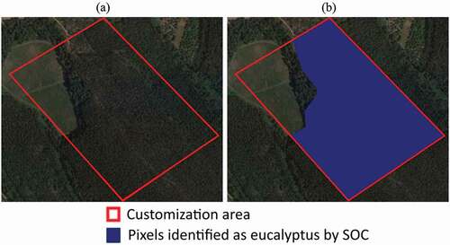
In this step, the customization area was chosen to perform: the data preparation; explain the rationale for our criteria selection (vegetation indices); and describe the bands used for performing the respective calculations. The customization area, outlined by the red polygon in Figure 2, is chosen because it includes a large eucalyptus plantation (visible by eye). It was opted to display the customization area inside its neighbourhood zone to show the region from where it was selected. Further, it is believed that the chosen customization area size (inside the red polygon) is enough to construct the normalized criteria for Eucalyptus classification and fusion of the various features. The customization area (red polygon) is shown in Figure 2, with the classification of eucalyptus (painted in blue) by the official Portuguese 2015 Chart of Soil Occupancy map (SOC 2015), which acts as ground-truth for the selection of aggregation operator to be used in the fusion process (step 3 in Figure 1).

Figure 2. Representation of the customization area located near the locality of Olival (39.697485, −8.588190). (a) The red line delineates the customization area, while the blue area (b) shows the pixels identified as eucalyptus by SOC

The criteria used for the data fusion approach were based on six different vegetation indices and Band 11 (directly from the Sentinel 2 Mission). The calculation of the vegetation indices was performed with a QGIS plugin (Raster calculator). Since some indices use bands with different resolutions, the Raster Calculator converts the output automatically in one single resolution and (e.g. in our case produced 10 × 10 pixel resolution images for all indices). The justification and details about the seven criteria (6 VI and 1 Band) for this approach are the following:

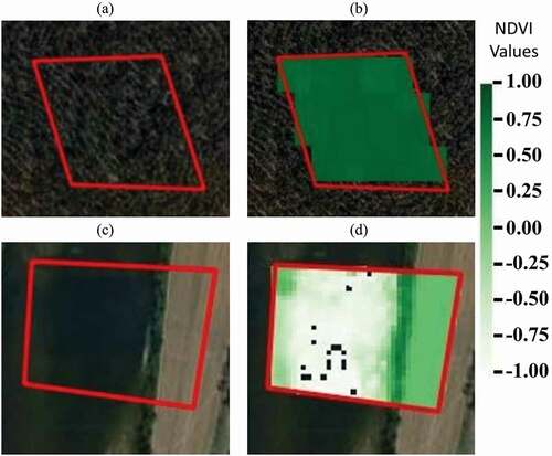
NDVI – The Normalized Difference Vegetation Index (NDVI) measures vegetation health, i.e. green vegetation (Rouse et al. 1973). Inputs used: Band 8 (Near-infrared – NIR) and Band 4 (Red), both with 10 m resolution. When eucalyptus reach adult age (and are healthy), they display the behaviour of very dense forests with dense green leaves; hence, NDVI helps to identify them when values are closer to +1. Figure 3 depicts an example of the NDVI response to two different kinds of land (see red polygons). In Figure 3, the corresponding NDVI values are shown on the right. The top example corresponds to a land with eucalyptus trees (values tending to +1), while bottom example represents water (values near −1) and agriculture fields.

Figure 3. Differences in NDVI index for different types of land cover based on the selection of the areas within the red polygons (a) area with eucalyptus forest; (b) NDVI values of area (a); (c) area with water agriculture fields; (d); NDVI values of the area (c) (source: QGIS 3.4.5)

CIG – Green Chlorophyll Index (CIG) estimates the chlorophyll content in leaves and studies have shown that eucalyptus display a relevant value of chlorophyll content (Coops et al. 2003); therefore, a high value for this index indicates a high chance of Eucalyptus Trees. Inputs used: Band 9 (Near Infrared – NIR), with 60 m resolution, and Band 3 (Green) with 10 m resolution. By experimentation on the customization area, the best values for identifying eucalyptus trees are in the range [9,11].

GNDVI – Green Normalized Difference Vegetation Index is relatively similar to NDVI but index it is more sensitive to chlorophyll content than NDVI (Gitelson, Kaufman, and Merzlyak 1996). Inputs used: Band 9 (NIR) with 60 m resolution, and Band 3 (Green) with 10 m resolution. For this index, the best customization values to identify eucalyptus trees were in the range [0.76, 0.86].

GVMI – Global Vegetation Moisture Index provides information about the vegetation water content from an area (Ceccato, Flasse, and Jean-Marie 2002). Since eucalyptus are trees with high water consumption levels (Liu and Jianhua 2010), as well as leaf water content (Datt 1999), this index can be very useful to identify them. Inputs used: Band 9 (NIR), with 60 m resolution and Band 12 (Short-wave infrared – SWIR), with 20 m resolution. Best range of values: [0.39,0.71].

NDMI – Normalized Density Moisture Index describes the crop’s water stress level and is calculated with a ratio between the difference and the sum of the refracted radiations in the NIR and SWIR. NDMI recognizes areas of vegetation with water stress problems. Inputs used: Band 8 (NIR), with 10 m resolution and Band 11 (SWIR), with 20 m resolution. Best range of values: [0.2, – 0.5].

SCI – Soil Composition Index is used to differentiate between soil and vegetation. In the proposed work, this index is very useful to remove data that is not vegetation (roads, cultivated fields, etc.). Inputs used: Band 11 (SWIR) and Band 8 (NIR), with resolution of 20 m and 10 m, respectively. Best range of values: [−0.35, – 0.25].

B₁₁ – This last chosen feature is the only one that is not a vegetation index. It refers to source data, retrieved directly from the spectral Band 11 of Sentinel 2 satellite. Even though it has limited cloud penetration, it is quite useful for measuring the moisture content of vegetation and it provides good contrast between different types of vegetation – a very important measure for eucalyptus identification. Its central wavelength is found at 1610 nm (Sinergise Laboratory for geographical information systems 2021). Band 11 has 20 m resolution customization; the best range of values were in the [0.08, 0.12] region.

5.2. Step 2 – fuzzy normalization

This step corresponds to the transformation of the input data domain into normalized numerical and comparable data, i.e. taking in account all features selected the normalization process transforms each area, corresponding to each feature into the [0,1] domain, using a membership function. After normalization, each pixel value, of any feature, will have a corresponding membership value, where high values are the best classified pixels and membership values close to zero correspond to worst classified pixels. To perform this step, the selected customization area is used (see Figure 3), from where the fuzzy membership functions are built. For this purpose, the topology for the membership functions that best represent the selected criteria are defined. Since six different vegetation indices (input data) and one band are used, the normalization process is executed for each one, resulting in seven membership functions of normalized data. To normalize each feature, three types of function were used, Sigmoid, Gaussian and Trapezoidal, depending on how well they fitted the input data from the images. The choice of membership functions topologies was based on the retrieving, for each index, of the pixel values that are eucalyptus trees, which allowed the building of their variance interval (domain). A summary of the membership functions used and their respective parameters for each criterion is depicted in Table 1.

Table 1. Membership functions used and their respective parameters for each input variable. SD stands for Standard Deviation

Variable	Range	Method	Parameter
NDVI	[0.4877,0.9025]	Sigmoid	Offset = 0.75 Width = 30
CIG	[2.3402,12.7055]	Trapezoidal	a (lower limit) = 7 b (upper limit) = 9 c (upper support limit) = 11  d (lower support limit) = 14
GNDVI	[0.53919,0.86399]	Sigmoid	Offset = 0.76 Width = 30
GVMI	[0.3577,0.7146]	Sigmoid	Offset = 0.39 Width = 30
NDMI	[−0.0233,0.4954]	Sigmoid	Offset = 0.2 Width = 30
SCI	[−0.4954,0.0233]	Gaussian	Mean = – 0.28 SD = 0.25
B11	[0.0666,0.2031]	Gaussian	Mean = 0.1 SD = 0.05

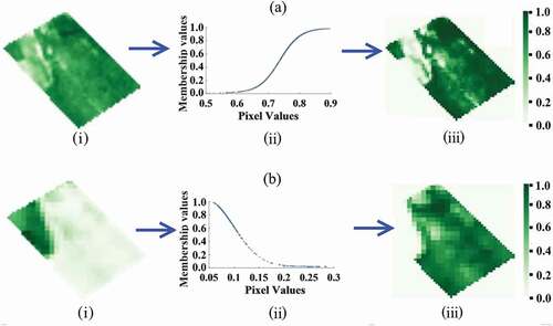
In the cases where sigmoid functions are applied (NDVI, GNDVI, GVMI, NDMI), the membership values are always increasing, i.e. the value was set as offset of the sigmoid function. For the Gaussian membership functions, the process was different (Indices SCI and B₁₁), as, for example, regarding the B₁₁ values, the pixels classified as ‘good’ membership values fall within the variation interval (0.08 to 0.12) and then higher values (like 0.15) refer to areas should not be assigned as eucalyptus. Due to this, the Gaussian membership function is appropriate because the membership value increases until its centre values (mean) and then starts to decrease, which was exactly the desired representation for SCI and B₁₁.

Table 1 summarizes the fuzzy normalization (step 2 of the data fusion approach) applied to the customization area for the seven criteria used and Figure 4 illustrates the process for two criteria, NDVI and B₁₁, with the original image on the left, its respective membership function (centre) and the normalized image (right). The manual customization process was done once with this approach, using the customization area, and then it was applied to classification of Eucalyptus trees in other validation areas.

Figure 4. Examples of normalization process for (a) NDVI sigmoidal membership function and (b) band 11 Gaussian membership function going from the (i) raw original image, through the process of normalization using the (ii) membership function and finally obtaining the (iii) normalized image (source: QGIS 3.4.5)

5.3. Step 3 – data fusion

This step consists in the fusion of the obtained normalized data to create a single added-value image with highlighted Eucalyptus trees. As mentioned before, the results were tested and compared with seven different aggregation operators from the three classes (non-parametric, average and reinforcement): (i) Max; (ii) Mean; (iii) Weighted Averaging; (iv) Weighting Functions; (v) Continuous Reinforcement Operator (CRO); (vi) Multiplicative FIMICA; (vii) Additive FIMICA.

This comparison allows us to customize the best aggregation operator to classify Eucalyptus. To perform the comparison, the SOC (Soil occupancy maps) was used as a ground truth (see Figure 5). With these ground truth data, the validation (percentage of correct classifications) was performed, for each aggregation operator. Hence, for each aggregation operator, it is counted how many pixels match the ground truth data, resulting on a percentage of hit and missed pixels, as follows:

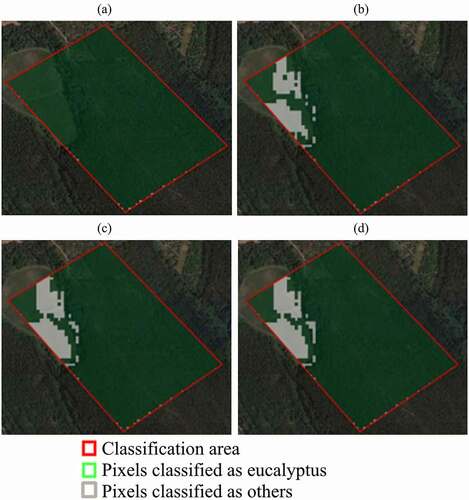
Figure 5. Example of the results of non-parametric operators: (a) max; (b) mean; (c) weighted average; (d) weighting functions. The green area shows the pixels identified as eucalyptus by each operator, while the white area shows the pixels identified as ‘others’. The customization was done within the red polygon area, as shown previously in Figure 3 located near the locality of Olival (39.697485, −8.588190) (source: QGIS 3.4.5, 2019)

Hit Rate (HR) – Measures the number of pixels classified correctly, i.e. that matched the ground truth data.

Miss Rate (MR) – Measures the rate of misclassified pixels, i.e. pixels that are classified as eucalyptus by the respective aggregation operator but SOC (ground-truth) classified them as non-eucalyptus.

In the next two sub-sections, the graphical results obtained for all seven operators are presented, divided into non-parametric operators and reinforcement operators. The selection of the best operator to perform data fusion with the aim of classifying Eucalyptus is discussed afterwards.

5.3.1. Graphical results for all operators

To facilitate discussion, the HR and MR results are presented for the non-parametric operators in graphical format (Figure 5) as well as for the parametric ones (Figure 6). Afterwards, in Section 5.3.2., the numerical results for each operator are presented with the corresponding best aggregation operator for this case study.

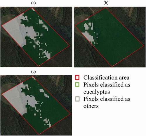
Figure 6. Example of the results of parametric operators (reinforcement operators), (a) CRO, (b) additive FIMICA and (c) multiplicative FIMICA on the example customization area which is located near the locality of Olival (39.697485, −8.588190); The green area shows the pixels identified as eucalyptus by each operator, while the white area shows the pixels identified as ‘others’. The customization was done within the red polygon area, as shown previously in Figure 3 (source: QGIS 3.4.5, 2019)

As can be seen in Figure 5(a), the max operator classified almost all pixels as Eucalyptus, which is clearly not a good result. Figure 5(b) shows the use of the mean operator, where it is already possible to distinguish some spots classified as non-eucalyptus (grey areas) and others positively as Eucalyptus (green areas).

The usage of the weighted average operator is shown in Figure 5(c), where the weights for each criterion involved were assigned by visual analysis of the normalized images for each index and taking into account which pixels are eucalyptus trees (SOC). The values of the weights that were used to create Figure 5(c) were 0.3 to NDMI index, 0.2 to CIG index, and 0.1 to the rest. Note that the sum of the weights must be equal to 1 (0.3 × 1.0 index + 0.2 × 1.0 index + 0.1 × 5.0 indices = 1.0). With this operator, it is possible to observe that more correct classifications for non-eucalyptus are obtained.

The use of the Weighting Function operator can be observed in Figure 5(d). For this customization step, the used linear weighting functions, borrowed from (Ribeiro et al. 2014). More details about the weighting functions operator can be seen in (Ribeiro et al. 2014; Marques-Pereira and Ribeiro 2003).

Regarding our customization area, each index was assigned with a different relative weight from: ‘very important’ (linear weighting function interval [0.8, 1]) to NDMI index, ‘important’ (linear weighting function interval [0.6, 0.8]) to CIG and ‘low importance’ (linear weighting function interval [0.2, 0.3]) to the remaining input data (Ribeiro et al. 2014).

For each pixel of each criterion, its satisfaction value (from x-axis) is weighted with its respective weight from y-axis. Afterwards, using the respective weighting functions it is possible to obtain the results for this operator, as shown in Figure 5(d).

For the reinforcement operators, it is required to set the g parameter to a common value for all three used reinforcement operators. This parameter controls the reinforcement level by penalizing scores values below a certain threshold, i.e. the value of neutral element (parameter g) and rewarding values above. Table 2 depicts the results for the three reinforcement operators with g parameters from 0.1 to 0.9.

Table 2. Hit rate (HR) and Miss Rate (MR) based on the g parameter

g	Multiplicative FIMICA		Additive FIMICA		CRO
	HR	MR	HR	MR	HR	MR
0.1	0.829	0.158	0.989	0.641	0.785	0.155
0.2	0.829	0.158	0.984	0.538	0.752	0.155
0.3	0.829	0.158	0.966	0.452	0.715	0.152
0.4	0.829	0.158	0.942	0.333	0.694	0.147
0.5	0.826	0.158	0.869	0.194	0.672	0.144
0.6	0.820	0.158	0.714	0.147	0.659	0.144
0.7	0.790	0.155	0.402	0.102	0.642	0.144
0.8	0.719	0.152	0.002	0.000	0.631	0.144
0.9	0.568	0.138	0.000	0.000	0.620	0.144

As can be seen in Table 2, for all reinforcement operators, the value g = 0.1 provided more hits because it ‘accepts’ most solutions, however, at the expense of higher missing values. Since in the case of eucalyptus, it is necessary to accept, as much as possible, good ‘solutions,’ this g value was chosen for the customization section.

The graphical results of the usage of reinforcement operators, CRO, Additive and Multiplicative FIMICA are shown, respectively, in Figure 6(a–c).

5.3.2. Selection of aggregation operator

In the previous sub-section, the obtained graphically set of results were presented (step 4 of the data fusion approach) for the customization area, through the application of all seven operators. Now, those results need to be compared to select which aggregation operator is more suitable for this work. The total of pixels classified as Eucalyptus in the SOC study area (ground-truth area) is 1088, while the non-eucalyptus classification is 360.

As can be seen in Table 3, most of the HR have an extremely high value (close to 1), which suggests that most operators correctly classified the eucalyptus. However, it is also imperative to minimize, as much as possible, the misclassified pixels. Therefore, the last column of Table 3 presents the ratio between the HR and MR, i.e. the difference between HR and MR.

Table 3. Comparative results for training area with ground-truth data (SOC classification). MR and HR stand for Miss Rate and Hit Rate, respectively

Operator	Number of hits	Number of misses	Miss rate	Hit rate	Ratio (Hit-Miss)
Max	1081	360	1.00	0.99	−0.01
Mean	1077	266	0.73	0.99	0.27
Weighted averaging	1077	244	0.67	0.98	0.31
Weighting function	1077	241	0.66	0.98	0.32
CRO	855	56	0.15	0.78	0.63
Additive FIMICA	1077	231	0.64	0.98	0.34
Multiplicative FIMICA	902	57	0.15	0.82	0.67

Max operator had the highest HR (as well as mean operator), but also has the highest total MR, i.e. it misclassified many pixels. Mean operator, despite presenting a lower MR than max, it is still very high for the intended goal. Regarding averaging operators, both (weighted average and weighting function) produced very similar results, along with Additive FIMICA. All three have very good HR but still very high missing rates, hence, resulting in a poor result.

CRO and Multiplicative FIMICA were the ones with the best results, having almost the same MR (56 and 57 misses, respectively). Regarding the number of hits, Multiplicative FIMICA had almost more 60 well-classified pixels, which means an improvement of 4% in relation to CRO.

Since, in classification problems, it is very important to balance the HR and MR, to ensure minimization of misclassified pixels, while maximizing the number of hits, it is possible to observe that the CRO and Multiplicative FIMICA operators have quite balanced results. However, since Multiplicative FIMICA has the highest ratio (0.67), it was chosen as the best aggregation operator for the data fusion approach.

From the comparison analysis above, on the customization area, the operator selected is FIMICA multiplicative. In the next section, several validations were performed to assess the suitability and versatility of our data fusion approach.

6. Results and discussion

This section presents the validation of the chosen operator (FIMICA multiplicative), using five other areas, selected from areas where it was possible to identify areas with eucalyptus trees (based on the SOC maps). The chosen areas had in mind different coverage of other representative cases. The same procedure is used to validate the data fusion approach as in the previous section (HR and MR). Notice that, again, the SOC images correspond to the ground-truth provided by DGT. All images have been acquired from tiles taken at 24 February 2019.

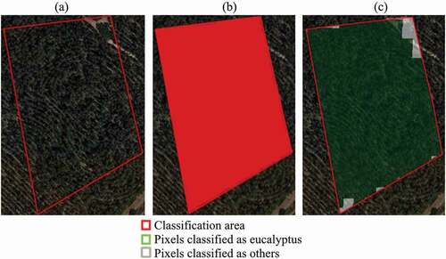
Figure 7 shows the chosen validation area for Scenario 1. In this validation example, an area only with Eucalyptus trees (according to SOC classification), the tested results are rather positive with an HR of 98% and an MR: 0% (since all pixels correspond to eucalyptus). There were some misclassified pixels of eucalyptus trees in the ground-truth map (grey areas) due to SOC assumption of 1 ha assuming the same classification. That is, according to SOC, there is only one kind of tree (eucalyptus) in the tested area; however, by simple visualization, it is possible to visualize that grey areas include other types of land. The MR is 0% because all pixels, classified as Eucalyptus by our approach, correspond to classified Eucalyptus in the SOC area. This test clearly shows that our automated process is more sensitive than the manual classification of SOC (due to the 1 ha assumption) and can distinguish eucalyptus from other types of land.

Figure 7. Validation of scenario 1 using the FIMICA multiplicative operator. Area near the village of Vila Nova de São Pedro, belonging to the municipality of Azambuja (39.201693, – 8.809251). (a) Original raw image with validation area (b) SOC classification; (c) classification using the FIMICA multiplicative operator. The green area shows the pixels identified as eucalyptus, while the white area shows the pixels identified as ‘others’. (source: QGIS 3.4.5, 2019)

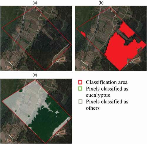
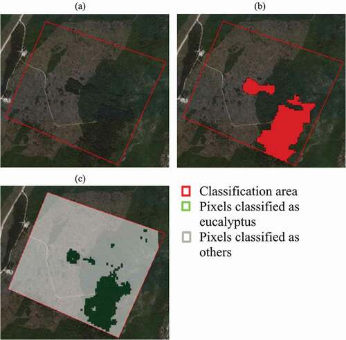
Figure 8 shows the chosen validation area for Scenario 2 (an example with a large forest of Eucalyptus, but also has a large area of roads and different types of vegetation), producing interesting results, where almost all eucalyptus were rightly classified (HR of 90%) while maintaining a relatively low missing rate (12%).

Figure 8. Validation of scenario 2 using the FIMICA multiplicative operator. Area near the village of Alcobertas, belonging to the municipality of Rio Maior (39.408168, −8.917378). (a) Original raw image with validation area; (b) SOC classification; (c) classification using the FIMICA multiplicative operator. The green area shows the pixels identified as eucalyptus, while the white area shows the pixels identified as ‘others’ (source: QGIS 3.4.5, 2019)

A third scenario is shown in Figure 9, which shows several eucalyptus areas divided by other types of lands. The chosen areas present big diversity of land (roads, eucalyptus, non-eucalyptus trees, etc.) and in both cases, the pixels assigned as eucalyptus by the proposed approach are matching the boundaries of the area delimited by SOC. Although it seems the obtained result is not that acceptable, it shows a very interesting outcome, inside the yellow circle, there is a road that separates two mini eucalyptus forests, but SOC marks them as eucalyptus (because the road separation is smaller than 1 ha), when they are not. With this result, it is believed that the value-added maps automatically produced in this work can provide additional resolution to the ones produced by the SOC manual process.

Figure 9. Validation of scenario 3 using the FIMICA multiplicative operator. Area is near the village of Vila Nova de São Pedro, belonging to the municipality of Azambuja (39.195977, −8.799908). (a) Original raw image with validation area; (b) SOC classification; (c) classification using the FIMICA multiplicative operator. (d) The yellow circle shows the road that intercepts the eucalyptus forest, which is not identified in SOC. The green area shows the pixels identified as eucalyptus, while the white area shows the pixels identified as ‘others’ (source: QGIS 3.4.5, 2019)

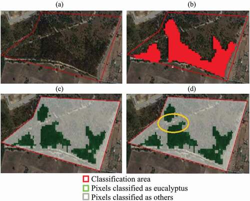
Figure 10 shows the validation area for Scenario 4. This example shares almost the same characteristics as the previous one, i.e. the manual process of SOC classified as eucalyptus areas where does not exist eucalyptus. HR: 76% MR: 0.1%. Both examples (Scenario 3 and 4), although presenting fewer HR when compared with the other ones, again demonstrate that our automated approach can be very useful for the identification of eucalyptus trees, separating elements that are not eucalyptus.

Figure 10. Validation of scenario 4 using the FIMICA multiplicative operator. Area near the village of Alcobertas, belonging to the municipality of area is in the municipality of Rio Maior (39.385998, −8.938425). (Source: QGIS 3.4.5, 2019). (a) Original raw image with validation area; (b) SOC classification; (c) Classification using the FIMICA multiplicative operator. The green area shows the pixels identified as eucalyptus, while the white area shows the pixels identified as ‘others’ (source: QGIS 3.4.5, 2019)

After the initial Validation with specific scenarios, a final example from an entire tile obtained directly from Sentinel (with 10,980 × 10,980 pixels at a resolution of 10 m), with the identification T295SNC_20190224T112111 (taken at 24 February 2019). Table 4 presents the confusion matrix for this tile along with the overall accuracy, user’s accuracy, producer’s accuracy, calculated as in (Olofsson et al. 2014). These results are at a similar level of the ones reported recently by (Forstmaier, Shekhar, and Chen 2020), using an approach based on Artificial Neural Networks (lower sensitivity: 69.61% compared to 75.70%, but higher specificity and overall accuracy, 99.43% compared to 95.80% and 98.19% compared to 92.50%).

Table 4. Confusion Matrix for the test tile (10,980 × 10,980) with the identification T295SNC_20190224T112111 (taken at 2019/02/24)

	Reference
Model		Eucalyptus	Non-Eucalyptus	Total	User’s accuracy (%)	Producer’s accuracy (%)
	Eucalyptus	3,022,068	662,606	3,684,674	82.02	69.61
	Non-Eucalyptus	1,319,349	115,356,377	116,875,726	99.13	99.43
	Total	4,341,417	116,218,983	120,560,400

7. Conclusions

In this work, a fuzzy-fusion approach was developed for land cover classification from multispectral satellite images, more specifically, for eucalyptus trees identification. The main objective was to fuse spectral information from a multispectral satellite imagery source (Sentinel 2 images) to produce a single compound for classification of a specific type of forest, the Eucalyptus.

Seven aggregation operators were compared to choose which is the most suitable for our customization set. The multiplicative FIMICA operator was found to be the most consistent operator and had the best classification outputs. After several validations were performed on other areas with different landscapes, to assess the approach suitability for automatic land cover identification, the results demonstrated that our automatic data fusion approach could be used to automatically identify eucalyptus forests, handling heterogeneous data, normalizing it, and producing fused information, ready for supporting effective decision-making.

Summarizing it is believed the data fusion approach, discussed in this work, produced very compelling results, concerning classification of eucalyptus forest areas, and it seems a robust automated process that can surpass timely manual classifications.

As future work, we plan to improve the customization process by using other customization areas and other criteria, to allow tuning the normalized functions to better fit identification of eucalyptus trees to improve the sensitivity of the algorithm. Another future work will be to compare the results of our approach with other available algorithms (e.g. random forests and decision trees), to assess its computational time, performance and accuracy for identification of Eucalyptus. Based on the comparison of an Artificial Neural Network approach (Forstmaier, Shekhar, and Chen 2020), it will probably be necessary to add other bands our algorithm, which will require more tuning. Furthermore, we also plan to apply this approach to other kinds of forests and other land types. These future works are part of the ongoing project IPSTERS (CA3-UNINOVA 2019) that partially financed this work.

Disclosure statement

No potential conflict of interest was reported by the authors.

Additional information

Funding

This work was supported by Portuguese Agency “Fundação para a Ciência e a Tecnologia“ (FCT), in the framework of projects PEST (UIDB/00066/2020) and IPSTERS (DSAIPA/AI/0100/2018)

References

- Ali, S. S., P. Dare, and S. D. Jones. 2008. “Fusion of Remotely Sensed Multispectral Imagery and Lidar Data for Forest Structure Assessment at the Tree Level.” ISPRS Proceedings, Beijing, 37. Citeseer: B7.
- Antrop, M. 2004. “Landscape Change and the Urbanization Process in Europe.” Landscape and Urban Planning 67 (1): 9–26. doi:10.1016/S0169-2046(03)00026-4.
- Ardeshir Goshtasby, A., and S. Nikolov. 2007. “Guest Editorial: Image Fusion: Advances in the State of the Art.” Information Fusion 8 (2): 114–118. Elsevier Science Publishers BV.
- Ayhan, E., and O. Kansu. 2012. “Analysis of Image Classification Methods for Remote Sensing.” Experimental Techniques 36 (1): 18–25. John Wiley & Sons, Ltd. doi: 10.1111/j.1747-1567.2011.00719.x.
- Baumgardner, M. F., F. S. LeRoy, L. L. Biehl, and E. R. Stoner. 1986. “Reflectance Properties of Soils”. In Advances in Agronomy, edited by, N C B T - Advances in Agronomy Brady, Vol. 38, 1–44. Cambridge, Massachusetts, USA: Academic Press. doi: 10.1016/S0065-2113(08)60672-0.
- Beliakov, G., A. Pradera, and T. Calvo. 2007. Aggregation Functions: A Guide for Practitioners. Vol. 221. Edited by K. Janusz. Berlin Heidelberg New York: Springer.
- Beliakov, G., and J. Warren. 2001. “Appropriate Choice of Aggregation Operators in Fuzzy Decision Support Systems.” IEEE Transactions on Fuzzy Systems 9 (6): 773–784. doi:10.1109/91.971696.
- Ben-Dor, E., Y. Inbar, and Y. Chen. 1997. “The Reflectance Spectra of Organic Matter in the Visible Near-Infrared and Short Wave Infrared Region (400–2500 Nm) during a Controlled Decomposition Process.” Remote Sensing of Environment 61 (1): 1–15. doi:10.1016/S0034-4257(96)00120-4.
- Bleiholder, J., and F. Naumann. 2009. “Data Fusion”. ACM Computing Surveys 41(1). New York, NY, USA: Association for Computing Machinery. doi:10.1145/1456650.1456651.
- Bourdarias, C., P. Da-Cunha, R. Drai, F. S. Luıs, and R. A. Ribeiro. 2010. “Optimized and Flexible Multi-Criteria Decision Making for Hazard Avoidance.” In Proceedings of the 33rd Annual AAS Rocky Mountain Guidance and Control Conference, Breckenridge, CO, USA, 5–10. Citeseer.
- CA3-UNINOVA. 2019. “IPSTERS (Ipsentinel Terrestrial Enhanced Recognition System).” https://www.ca3-uninova.org/project_ipsters.
- Calvo, T., G. Mayor, and R. Mesiar. 2012. Aggregation Operators: New Trends and Applications. Vol. 97. Physica. New York, USA.
- Câmara, F., J. Oliveira, T. Hormigo, J. Araújo, R. Ribeiro, A. Falcão, M. Gomes, O. Dubois-Matra, and S. Vijendran. 2015. “Data Fusion Strategies for Hazard Detection and Safe Site Selection for Planetary and Small Body Landings.” CEAS Space Journal 7 (2): 271–290. doi:10.1007/s12567-014-0072-y.
- Campanella, G., and R. A. Ribeiro. 2011. “A Framework for Dynamic Multiple-Criteria Decision Making.” Decision Support Systems 52 (1): 52–60. doi:10.1016/j.dss.2011.05.003.
- Ceccato, P., S. Flasse, and G. Jean-Marie. 2002. “Designing a Spectral Index to Estimate Vegetation Water Content from Remote Sensing Data: Part 2. Validation and Applications.” Remote Sensing of Environment 82 (2): 198–207. doi:10.1016/S0034-4257(02)00036-6.
- Chang, N.-B., and K. Bai. 2018. Multisensor Data Fusion and Machine Learning for Environmental Remote Sensing. 1st ed. Boca Raton, USA: CRC Press.
- Colditz, R. R. 2015. “An Evaluation of Different Training Sample Allocation Schemes for Discrete and Continuous Land Cover Classification Using Decision Tree-Based Algorithms.” Remote Sensing. doi:10.3390/rs70809655.
- Coops, N. C., C. Stone, D. S. Culvenor, L. A. Chisholm, and R. N. Merton. 2003. “Chlorophyll Content in Eucalypt Vegetation at the Leaf and Canopy Scales as Derived from High Resolution Spectral Data.” Tree Physiology 23 (1): 23–31. doi:10.1093/treephys/23.1.23.
- Dai, X., and S. Khorram. 1999. “Data Fusion Using Artificial Neural Networks: A Case Study on Multitemporal Change Analysis.” Computers, Environment and Urban Systems 23 (1): 19–31. doi:10.1016/S0198-9715(98)00051-9.
- Datt, B. 1999. “A New Reflectance Index for Remote Sensing of Chlorophyll Content in Higher Plants: Tests Using Eucalyptus Leaves.” Journal of Plant Physiology 154 (1): 30–36. doi:10.1016/S0176-1617(99)80314-9.
- Davidson, N. C., and C. M. Finlayson. 2007. “Earth Observation for Wetland Inventory, Assessment and Monitoring.” Aquatic Conservation: Marine and Freshwater Ecosystems 17 (3): 219–228. John Wiley & Sons, Ltd. doi: 10.1002/aqc.846.
- Desclée, B., P. Bogaert, and P. Defourny. 2006. “Forest Change Detection by Statistical Object-Based Method.” Remote Sensing of Environment 102 (1): 1–11. doi:10.1016/j.rse.2006.01.013.
- Fauvel, M., J. Chanussot, and J. A. Benediktsson. 2006. “Decision Fusion for the Classification of Urban Remote Sensing Images.” IEEE Transactions on Geoscience and Remote Sensing 44 (10): 2828–2838. doi:10.1109/TGRS.2006.876708.
- Forstmaier, A., A. Shekhar, and J. Chen. 2020. “Mapping of Eucalyptus in Natura 2000 Areas Using Sentinel 2 Imagery and Artificial Neural Networks.” Remote Sensing 12 (14): 4–6. doi:10.3390/rs12142176.
- Friedl, M. A., and C. E. Brodley. 1997. “Decision Tree Classification of Land Cover from Remotely Sensed Data.” Remote Sensing of Environment 61 (3): 399–409. doi:10.1016/S0034-4257(97)00049-7.
- Gallego, F. J., and H. J. Stibig. 2013. “Area Estimation from a Sample of Satellite Images: The Impact of Stratification on the Clustering Efficiency.” International Journal of Applied Earth Observation and Geoinformation 22: 139–146. doi:10.1016/j.jag.2012.03.003.
- Garcia, H. 2017. “A Floresta Em Portugal. Causas E Consequências Da Expansão Do Eucalipto. Caso De Estudo: O Concelho De Torres Vedras.” Doctoral Dissertation - Universidade Nova de Lisboa, Faculdade de Ciências Sociais e Humanas.
- Ghamisi, P., B. Rasti, N. Yokoya, Q. Wang, B. Hofle, L. Bruzzone, F. Bovolo, et al. 2019. “Multisource and Multitemporal Data Fusion in Remote Sensing: A Comprehensive Review of the State of the Art.” IEEE Geoscience and Remote Sensing Magazine 7 (1): 6–39. doi:10.1109/MGRS.2018.2890023.
- Gitelson, A. A., Y. J. Kaufman, and M. N. Merzlyak. 1996. “Use of a Green Channel in Remote Sensing of Global Vegetation from EOS-MODIS.” Remote Sensing of Environment 58 (3): 289–298. doi:10.1016/S0034-4257(96)00072-7.
- Haywood, A., and C. Stone. 2011. “Semi-Automating the Stand Delineation Process in Mapping Natural Eucalypt Forests.” Australian Forestry 74 (1): 13–22. Taylor & Francis. doi: 10.1080/00049158.2011.10676341.
- Hsu, S.-L., P.-W. Gau, I.-L. Wu, and J.-H. Jeng. 2009. “Region-Based Image Fusion with Artificial Neural Network.” World Academy of Science, Engineering and Technology 53: 156–159.
- Hyder, A. K., E. Shahbazian, and E. Waltz. 2012. Multisensor Fusion. Vol. 70. Springer-Verlag New Yor.
- ICNF, Instituto da Conservação da Natureza e das Florestas. 2019. “6th Portuguese Forest Inventory (IFN6).” http://www2.icnf.pt/portal/florestas/ifn/ifn6.
- Jassbi, J. J., R. A. Ribeiro, L. M. Camarinha-Matos, J. Barata, and M. I. Gomes. 2018. “Continuous Reinforcement Operator Applied to Resilience in Disaster Rescue Networks.” In FUZZ-IEEE WCCI2018 Conference, July 8-13, Rio Janeiro, Brasil, 942–947. doi:10.1109/FUZZ-IEEE.2018.8491482.
- Jenicka, S. 2018. “Sugeno Fuzzy-Inference-System-Based Land Cover Classification of Remotely Sensed Images.” In Environmental Information Systems: Concepts, Methodologies, Tools, and Applications, 3:1247–1283.IGI Global. doi:10.4018/978-1-5225-7033-2.ch057.
- Kanellopoulos, I., and G. G. Wilkinson. 1997. “Strategies and Best Practice for Neural Network Image Classification.” International Journal of Remote Sensing 18 (4): 711–725. Taylor & Francis. doi: 10.1080/014311697218719.
- Klein, L. A. 2004. Sensor and Data Fusion: A Tool for Information Assessment and Decision Making. Vol. 138. Bellingham, Washington USA: SPIE press.
- Lavreniuk, M. S., S. V. Skakun, A. Ju, B. Shelestov, Y. Ya, S. L. Yanchevskii, D. J. U. Yaschuk, and A. Ì. Kosteckiy. 2016. “Large-Scale Classification of Land Cover Using Retrospective Satellite Data.” Cybernetics and Systems Analysis 52 (1): 127–138. doi:10.1007/s10559-016-9807-4.
- Le Maire, G., C. Marsden, W. Verhoef, F. J. Ponzoni, D. L. Seen, A. Bégué, J.-L. Stape, and Y. Nouvellon. 2011. “Leaf Area Index Estimation with MODIS Reflectance Time Series and Model Inversion during Full Rotations of Eucalyptus Plantations.” Remote Sensing of Environment 115 (2): 586–599. doi:10.1016/j.rse.2010.10.004.
- Lee, H., B. Lee, K. Park, and R. Elmasri. 2010. “Fusion Techniques for Reliable Information: A Survey.” International Journal of Digital Content Technology and Its Applications 4 (2): 74–88. Advanced Institute of Convergence IT.
- Li, Z., and X. Guo. 2015. “Remote Sensing of Terrestrial Non-Photosynthetic Vegetation Using Hyperspectral, Multispectral, SAR, and LiDAR Data.” Progress in Physical Geography: Earth and Environment 40 (2): 276–304. SAGE Publications Ltd. doi: 10.1177/0309133315582005.
- Liu, H., and L. Jianhua. 2010. “The Study of the Ecological Problems of Eucalyptus Plantation and Sustainable Development in Maoming Xiaoliang.” Journal of Sustainable Development 3 (1): 197–201. doi:10.5539/jsd.v3n1p197.
- Manyika, J., and H. Durrant-Whyte. 1995. Data Fusion and Sensor Management: A Decentralized Information-Theoretic Approach. New Jersey, USA: Prentice Hall PTR.
- Mardani, A., M. Nilashi, E. K. Zavadskas, S. R. Awang, H. Zare, and N. M. Jamal. 2018. “Decision Making Methods Based on Fuzzy Aggregation Operators: Three Decades Review from 1986 to 2017.” International Journal of Information Technology & Decision Making 17 (2): 391–466. World Scientific Publishing Co. doi: 10.1142/S021962201830001X.
- Marinelli, G. C. C., F. Dukatz, and R. Ferrati. 2008. “Artificial Neural Networks and Remote Sensing in the Analysis of the Highly Variable Pampean Shallow Lakes.” Mathematical Biosciences and Engineering 5 (4): 691–711. doi:10.3934/mbe.2008.5.691.
- Marques-Pereira, R., and R. A. Ribeiro. 2003. “Aggregation with Generalized Mixture Operators Using Weighting Functions.” Fuzzy Sets and Systems 137: 43–58. http://www.uninova.pt/ca3/en/docs/BJ23-FSS2003.pdf.
- Mas, J. F., and J. J. Flores. 2008. “The Application of Artificial Neural Networks to the Analysis of Remotely Sensed Data.” International Journal of Remote Sensing 29 (3): 617–663. Taylor & Francis. doi: 10.1080/01431160701352154.
- Mora, A., M. A. Tiago Santos, S. Łukasik, M. N. João Silva, J. António Falcão, M. José Fonseca, A. Rita Ribeiro, et al. 2017. “Land Cover Classification from Multispectral Data Using Computational Intelligence Tools: A Comparative Study.” Information 8 (4): 147. doi:10.3390/info8040147.
- Mora, A. D., A. J. Falcão, L. Miranda, R. A. Ribeiro, and J. M. Fonseca. 2015. “A Fuzzy Multicriteria Approach for Data Fusion.” In Multisensor Data Fusion from Algorithms and Architectural Design to Applications, edited by H. Fourati, 109–126. Boca Raton, USA: CRC Press.
- Mora, A. D., A. J. Falcão, L. Miranda, R. A. Ribeiro, and J. M. Fonseca. 2016. “A Fuzzy Multicriteria Approach for Data Fusion.” In Multisensor Data Fusion: From Algorithms and Architectural Design to Applications, edited by H. Fourati, 109–126, Taylor and Francis Group. Boca Raton, USA: CRC Press.
- Olofsson, P., G. M. Foody, S. V. Martin Herold, C. E. W. Stehman, and M. A. Wulder. 2014. “Good Practices for Estimating Area and Assessing Accuracy of Land Change.” Remote Sensing of Environment 148: 42–57. Elsevier Inc. doi:10.1016/j.rse.2014.02.015.
- Paliwal, M., and U. A. Kumar. 2009. “Neural Networks and Statistical Techniques: A Review of Applications.” Expert Systems with Applications 36 (1): 2–17. Elsevier Ltd. doi: 10.1016/j.eswa.2007.10.005.
- Piella, G. 2003. “A General Framework for Multiresolution Image Fusion: From Pixels to Regions.” Information Fusion 4 (4): 259–280. doi:10.1016/S1566-2535(03)00046-0.
- Piiroinen, R., J. Heiskanen, E. Maeda, A. Viinikka, and P. Pellikka. 2017. “Classification of Tree Species in a Diverse African Agroforestry Landscape Using Imaging Spectroscopy and Laser Scanning.” Remote Sensing. doi:10.3390/rs9090875.
- Reshmidevi, T. V., T. I. Eldho, and R. Jana. 2009. “A GIS-Integrated Fuzzy Rule-Based Inference System for Land Suitability Evaluation in Agricultural Watersheds.” Agricultural Systems 101 (1): 101–109. doi:10.1016/j.agsy.2009.04.001.
- Ribeiro, R. A., T. C. Pais, and L. F. Simões. 2010. “Benefits of Full-Reinforcement Operators for Spacecraft Target Landing BT - Preferences and Decisions: Models and Applications.” In Preferences and Decisions, edited by, S. Greco, R. A. M. Pereira, M. Squillante, R. R. Yager, and J. Kacprzyk, 353–367. Berlin, Heidelberg: Springer Berlin Heidelberg. doi: 10.1007/978-3-642-15976-3_21
- Ribeiro, R. A., A. Falcão, A. Mora, and J. M. Fonseca. 2014. “FIF: A Fuzzy Information Fusion Algorithm Based on Multi-Criteria Decision Making.” Knowledge-Based Systems 58 (March 2014): 23–32. doi:10.1016/j.knosys.2013.08.032.
- Ribeiro, R. A., and P. Ricardo Alberto Marques. 2003. “Generalized Mixture Operators Using Weighting Functions: A Comparative Study with WA and OWA.” European Journal of Operational Research 145 (2): 329–342. doi:10.1016/S0377-2217(02)00538-6.
- Ross, T. J. 2004. Fuzzy Logic with Engineering. Wiley, Second ed. New Jersey, USA.
- Rouse, J. W., Jr, R. Hect Haas, J. A. Schell, and D. W. Deering. 1973. Monitoring the Vernal Advancement and Retrogradation (Green Wave Effect) of Natural Vegetation – Technical Report.
- Rudas, I. J., E. Pap, and J. Fodor. 2013. “Information Aggregation in Intelligent Systems: An Application Oriented Approach.” Knowledge-Based Systems 38: 3–13. doi:10.1016/j.knosys.2012.07.025.
- Santos, T. M. A., R. A. Andre Mora, and M. N. S. Joao. 2016. “Fuzzy-Fusion Approach for Land Cover Classification.” In Proceedings of INES 2016-20th Jubilee IEEE International Conference on Intelligent Engineering Systems, June 30-July 2 2016, Hungary pp. 177–182. IEEE. doi:10.1109/INES.2016.7555116.
- Schmitt, M., and X. X. Zhu. 2016. “Data Fusion and Remote Sensing: An Ever-Growing Relationship.” IEEE Geoscience and Remote Sensing Magazine 4 (4): 6–23. doi:10.1109/MGRS.2016.2561021.
- Sinergise Laboratory for geographical information systems, Ltd. 2021. “Sentinel-2 Bands: Band 11.” https://www.sentinel-hub.com/eoproducts/band-b11.
- Somers, B., J. Verbesselt, E. M. Ampe, N. Sims, W. W. Verstraeten, and P. Coppin. 2010. “Monitoring of Defoliation in Mixed-Aged Eucalyptus Plantations Using Landsat 5-TM.” In EGU General Assembly Conference Abstracts, Vienna, Austria, 02 – 07 May 2010. 12:11449.
- Sumfleth, K., and R. Duttmann. 2008. “Prediction of Soil Property Distribution in Paddy Soil Landscapes Using Terrain Data and Satellite Information as Indicators.” Ecological Indicators 8 (5): 485–501. doi:10.1016/j.ecolind.2007.05.005.
- Taylor, J. C., T. R. Brewer, and A. C. Bird. 2000. “Monitoring Landscape Change in the National Parks of England and Wales Using Aerial Photo Interpretation and GIS.” International Journal of Remote Sensing 21 (13–14): 2737–2752. Taylor & Francis. doi: 10.1080/01431160050110269.
- Torra, V., and Y. Narukawa. 2007. Modeling Decisions - Information Fusion and Aggregation Operators In Cognitive Technologies. Springer, Heidelberg, Germa.
- Triantaphyllou, E. 2000. “Multi-Criteria Decision Making Methods“ In Multi-Criteria Decision Making Methods: A Comparative Study” by, E. Triantaphyllou, 5–21. Boston, MA: Springer US. doi: 10.1007/978-1-4757-3157-6_2
- Xu, M., P. Watanachaturaporn, P. K. Varshney, and M. K. Arora. 2005. “Decision Tree Regression for Soft Classification of Remote Sensing Data.” Remote Sensing of Environment 97 (3): 322–336. doi:10.1016/j.rse.2005.05.008.
- Yager, R. R., and A. Rybalov. 1998. “Full Reinforcement Operators in Aggregation Techniques.” Transactions on Systems, Man, and Cybernetics Part B 28 (6): 757–769. IEEE Press. doi: 10.1109/3477.735386.
- Yang, S., Q. Feng, T. Liang, B. Liu, W. Zhang, and H. Xie. 2018. “Modeling Grassland Above-Ground Biomass Based on Artificial Neural Network and Remote Sensing in the Three-River Headwaters Region.” Remote Sensing of Environment 204: 448–455. doi:10.1016/j.rse.2017.10.011.
- Zhang, L., and W. Xiaolin. 2006. “An Edge-Guided Image Interpolation Algorithm via Directional Filtering and Data Fusion.” IEEE Transactions on Image Processing 15 (8): 2226–2238. IEEE.