Estimation of global horizontal irradiance in China using a deep learning method

ABSTRACT

Quasi-real-time estimation of Global Horizontal Irradiance (GHI) is a key parameter for many solar energy applications. We propose the use of a deep belief network (DBN) to estimate GHI under all-sky conditions derived from Himawari-8 satellite images with a high accuracy and high efficiency, and a high spatial and time resolution for a large geographical area. The DBN solver for GHI (DBN-GHI) is based upon a radiative transfer model, Santa Barbara Discrete Ordinate Radiative Transfer (SBDART), to maintain the balance between computational efficiency and accuracy. The computational time of DBN-GHI for one satellite image with more than 400,000 pixels is around 9 seconds. Aerosol was considered as the main attenuation factor for clear skies, while cloud parameters were used for cloudy-sky GHI estimation. The main novelty of this research is that prior to it, there is a dearth of GHI estimations in China at minutely or hourly intervals in all sky conditions. The results of hourly comparison of this with ground-based observations gave a very good Pearson correlation coefficient (r), above 0.95, with a Root-Mean-Square-Error (RMSE) between about 30 to 80 w m⁻².

1. Introduction

The sun is the primary source of energy for the earth’s climate system. Accurate solar irradiance data at ground level is useful not only for the study of climate systems, for agriculture, meteorology applications and other applications and for efficient estimations of the surface solar radiation and photovoltaic (PV), a renewable and clean renewable energy source that plays an increasing role. A key component of solar radiation is Global Horizontal Irradiance (GHI), defined as the shortwave irradiance stemming from the sun on the Earth’s horizontal surface, the sum of the direct irradiance and the diffuse horizontal irradiance (Maxwell, Wilcox, and Rymes 1993).

It is beneficial to monitor PV power generation at a high rate (nearly 5 to 15 minutes) in order to control electric power systems safely for a stable supply–demand balance. So estimates for near-real-time decisions, linked to distributed grid-connected PV are needed (Kosmopoulos et al. 2018). PV power generated by residential and factory rooftop systems, and solar plants often has not been directly measured in real time, because PV power generation data cannot be accurately collected by its monitoring instruments. This is a serious safety issue for the control of electric power grids because it is not possible to accurately measure PV power generation under different weather conditions. Therefore, information on GHI in real time and/or on a quasi-real time scale has been required to improve the management of PV systems in power grids.

Ground-based measurements of solar irradiance using a pyranometer provide a simple and accurate way to gauge solar energy. However, the sparse network of pyranometers/stations cannot reliably estimate the variability of GHI in large spatial regions. Compared with the method for interpolation obtained from station measurements when the distance from the station exceeds 34 km for hourly irradiation and 50 km for daily irradiation, the overall accuracy of satellite-derived irradiance is higher (Perez, Seals, and Zelenka 1997).

Cloud, aerosols and water vapour contribute to the transparency of the atmosphere, therefore they alter the solar irradiance reaching the earth’s surface (Lin et al. 2015). Surface albedo that quantifies the fraction of the sunlight reflected by the surface also has an influence on solar irradiance (Gueymard et al. 2019). Physical parameters such as cloud optical thickness (COT), cloud phases and cloud effective radius. are considered to be useful to quantify the cloud’s influence on solar irradiance. Under cloudless condition, aerosols are the dominant factor for solar irradiance attenuation. A popular indicator of atmospheric pollutants is Aerosol optical thickness (AOT). The overall instantaneous direct forcing efficiency defined as the solar irradiance perturbation on the surface owing to aerosol changes, is in the range of a power per unit area of 120 to150 w m⁻² per unit of AOT (Damiani et al. 2018). All-sky conditions include cloudless and cloudy days. Due to the small number of polar orbiting-satellites that pass over East Asia such as Moderate Resolution Imaging Spectroradiometer (MODIS) and the spatial and spectral resolution of geostationary satellites such as MTSAT being more coarse-gained, East Asia had a relatively weak satellite coverage until recently. Hence, Himawari-8, was launched in 2015. This can be used to quantify solar irradiance at a high spatial and temporal resolution for most of China.

GHI estimation derived from satellite image methods are separated into 3 broad types: empirical, semi-empirical, and physical methods (Pinker, Frouin, and Li 1995). Empirical methods are usually associated with statistical regression between satellite observations and ground-based measurements. The difference between empirical and semi-empirical models concerns whether radiative transfer models (RTM) were utilized. The Heliosat method and its updated versions, e.g. (Beyer, Costanzo, and Heinemann 1996), are some of the most famous and widely used semi-empirical models.

Physical models generally use radiative transfer theory to calculate the surface irradiance, using the parameters retrieved through remote sensing, such as cloud properties, water vapour, aerosol optical thickness and ozone as inputs and others. Some examples are MODTRAN (Berk, Bernstein, and Robertson 1987), SBDART (Ricchiazzi et al. 1998) and FARMS (Xie, Sengupta, and Dudhia 2016).

Physical models can calculate irradiance accurately, which is an obvious advantage, if detailed vertical distributions of atmospheric components such as pressure, temperature, density, and volume mixing ratio for gases are known. However, some of these parameters are dynamic and hard to acquire.

Note, the computation time is considerably longer, compared with empirical and semi-empirical models (Antonanzas-Torres et al. 2019).

Several Artificial Intelligence (AI) techniques have been applied to produce solar irradiance estimates and for forecasting. Artificial Neural Network (ANN) with ground-observed data can be used to estimate Hourly global photosynthetically active radiation (PAR) in Spain. After that, estimating the hourly global irradiance, based on an ANN trained with data recorded by 15 observation stations in Spain and a satellite-derived cloud index, was published (Zarzalejo, Ramirez, and Polo 2005). These did not consider the radiative transfer theory and are similar to empirical methods. By contrast, the radiative transfer code ‘STREAMER’ can be sped up using an ANN with a back-propagation (BP) algorithm (Key and Schweiger 1998). A customized ANN solver stemmed from the RSTAR5b (Nakajima and Tanaka 1986), a kind of radiative transfer code, was employed to estimate downward and upward shortwave fluxes at the top of the atmosphere and at the surface efficiently (Takenaka et al. 2011). ANN radiative transfer solvers have been created based on LibRadtran (Mayer and Kylling 2005), to generate high-resolution solar irradiance spectra parameterized by cloud and aerosol parameters (Taylor et al. 2016).

It is computationally costly to estimate solar irradiance directly using an RTM from satellite data. This is why the trade-off between computational cost versus accuracy needs to be dealt with. One common way of reducing the computational burden is by means of creating off-line look-up tables (LUTs). Computation speed of LUTs-based approaches may be markedly reduced when a great amount of satellite images and large LUTs are used.

The goal of this study is to estimate real-time GHI using a deep learning method, called a deep belief network (DBN). A deep belief network (DBN) is a generative graphical model, composed of multiple layers of hidden units. The hidden units of different layers are connected but no connection exists within the same layer (Hinton and Osindero 2006). The proposed benefits of using a DBN is that the quick and accurate extraction of samples’ essential features is available. The advantages of unsupervised learning and supervised learning are combined, and it is a good approach because of its recognition ability for big data.

In our proposed method, a geostationary satellite, Himawari-8, is a key data resource to perform a quasi-real-time estimation of GHI, for an area without adequate ground-observations. Because of the reduction in the number of such surface monitoring equipment, a cost-saving results. This is the first research on GHI estimates using satellite images and the use of a deep belief network.

Our main contribution is to research and develop the application of a deep belief network (DBN) to estimate GHI under all-sky conditions derived from Himawari-8 satellite images with a high accuracy and high efficiency and a relatively high spatial and temporal resolution, for a large geographical area. Engineers or scientists could use this model to perform a quasi‐real‐time estimation of PV power potential at a uniform horizontal resolution, even for regions with no surface GHI instruments. This would allow for increased cost savings because the amount of surface monitoring equipment would be reduced.

According to the common radiative transfer theory, which is suitable for the atmosphere on the earth, the proposed model can be used in other regions of the world, if the inputs can be known.

This research proposed a new method in estimating solar energy potential at a high temporal frequency. In addition, due to the lack of attention to air pollution or haze, many previous models fail to obtain reliable GHI estimates in areas with severe and changing air pollution concentrations. A high AOT, which is recognized as a common indicator of air pollution, is responsible for the reduction of solar energy by absorbing and scattering light. Li et al. (2017) revealed that aerosol pollution in China greatly reduces surface solar PV resources over both northern and eastern China. This study also contributes to decrease the uncertainty of GHI estimate under air pollution conditions, especially in northern China.

2. Data used

We used multi-sourced data including Himawari-8 observations, MODIS land surface products, reanalysis data and others. Due to use of a radiative transfer model, the inputs of the training datasets represent atmospheric, and surface properties, need to be imported into the RTM. The output of training datasets is the GHI calculated by RTM. The design of training datasets follows that of (Takenaka et al. 2011) and (Taylor et al. 2016). All of input data are resampled to the resolution of 5 km, the same as the output results.

2.1. Ground-based GHI data

The Chinese Ecosystem Research Network (CERN) is an ecosystem research network with field stations throughout China (Fu et al. 2010). GHI, as one of the most important surficial parameters, is measured by a Kipp & Zonen CM11 pyranometer at 36 CERN stations across China. Though CERN possesses 36 stations, only 19 stations offer hourly GHI records through the official website in 2016. The selected CERN stations are shown in Figure 1. In this study, we use the measured records on August 21, August 25, November 1, November 4, to compare with our estimates.

Figure 1. Spatial distribution of selected sites of e CERN

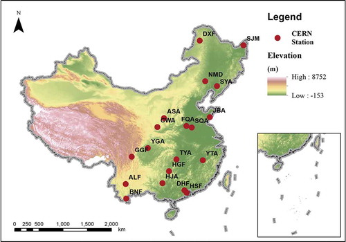
These days were chosen randomly. The aim of this research is to introduce a method rather than to produce and provide a solar irradiance database for one year. In addition, Himawari-8 satellite can capture more than 48 images over China a day, meaning more than 20 GB a day. China covers an area of around 9.6 million km², which means that the weather conditions were widely varied on different areas within a date. Some extreme weather conditions may cause this to be invalidated because the uncertainty of the input dataset. For example, extreme weather may cause a failure to retrieve the cloud optical depth, provided by the Japan Aerospace Exploration Agency.

2.2. Himawari-8 cloud property products

With a temporary resolution of 10 minutes, Japan Aerospace Exploration Agency (JAXA) has provided data comprised cloud mask, cloud optical thickness (COT), cloud effective radius (CER), Cloud phase and other parameters with a spatial resolution of 0.05° × 0.05°. Cloud mask identifies clear-sky and cloudy-sky pixels. Cloud phase recognizes whether or not a cloudy pixel represents ice cloud, water cloud pixel or mixed cloud (with a composition lying between a water cloud and ice cloud). COT and CER quantify the attenuation of incoming solar radiation. We chose 2 days both in summer and winter randomly: 21 August 2018, 25 August 2018, 1 November 2018 and 4 November 2018.

2.3. Ancillary input data

In this study, the surface shortwave broadband (0.4 to 2.2 μm) albedo product (Deneke, Feijt, and Roebeling 2008) MCD43C31 (MODIS) is employed, defined as albedo when the diffuse component is isotropic and the direct component is absent. Minutely AOT is retrieved by a new algorithm which use the ratio of Himawari-8 visible band (Xiaojun et al. 2019).

Some aerosol physical parameters such as Single scattering albedo (SSA) and Angstrom Exponent (AE) cannot be obtained directly from Himawari-8 observations. MOD08, the monthly averaged Level 3 aerosol product at 1° × 1° horizontal resolutions, supply these parameters. Moreover, total column water vapour data, extracted from CERA-SAT reanalysis dataset on 0.125° grid, is also employed as inputs to the model. The global 1 km NASA Shuttle Radar Topography Mission data (SRTM) is used to represent the surface elevation required for the estimate of GHI.

3. Methodology

This section presents an overview of the estimation model, it estimates the GHI using a deep belief network (denoted as DBN-GHI). In this study, DBN-GHI model is based on the calculation results of a radiative transfer model, Santa Barbara Discrete Ordinate Radiative Transfer (SBDART).

3.1. Overview of the deep belief network

A deep artificial neural network (ANN) is a numerical model of neuron network, containing many nonlinear processing layers and some characteristics that is used in AI applications such as natural language processing, pattern recognition and voice and speech analysis.

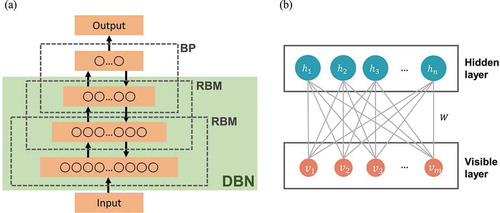
This overcomes some key limitations with ‘non-deep’ ANNs such as the Multilayer Perceptron and Radial basis function networks whose training is time-consuming, and which are more easily trapped at local minima. To deal with these limitations, a DBN (Deep Belief Network) that includes more hidden layers was created (Schmidhuber 2015). A common DBN is comprised of multiple restricted Boltzmann machine (RBM) layers and a back-propagation (BP) layer, aimed at addressing classification or regression problems. A simple structure of a DBN with two RBM layers is shown in (Figure 2(a,b)). The details of the structure of DBN are shown in the next section. Layers of DBN are created from a Restricted Boltzmann Machine (RBM), which is a generative and undirected probabilistic model.

Figure 2. The structure of an ordinary DBN and diagram of a restricted Boltzmann machine. (a) A simple structure of a DBN; (b) A simple structure of a RBM

3.2. Structure and training of a restricted Boltzmann machine

After being trained without supervision by RBMs, the probability distribution over its set of inputs can be learnt, which means that the weights of multi-layer neural networks can be initialized. Indeed, most of improvements in DBNs are due to improvements in RBMs. RBMs are a variant of Boltzmann machines, as their name implies. Their neurons must form a bipartite graph, which are commonly referred to as the ‘visible’ and ‘hidden’ units, respectively. Connections between different group are available, with the absence of connections between nodes within a group.

The succinct type of RBM consists of binary-valued hidden units $h_j$ and visible units $v_i$, and have a matrix of weights $w_{i,j}$ associated with the connection between a hidden unit $h_j$ and a visible unit $v_i$, where $m$ and $n$ are the number of visible units and the number of hidden units, respectively. Bias weights are assigned as $b_j$ to the hidden units and assigned as $a_i$ to the visible units.$\mathit{v},$ $\mathit{h},\mathit{a}$ and $\mathit{b}$are vectors. Hence, after adding this bias to this type of RBM, its energy of a configuration $\left(\mathit{v},\mathit{h}\right)$ is defined in Equation (1)(1) $\begin{array}{c}E\left(\mathit{v},\mathit{h}\right)=-{\mathit{v}}^{\mathbf{T}}Wh-{\mathit{a}}^{\mathbf{T}}v-{\mathit{b}}^{\mathbf{T}}h\\ =-\sum _{i=1}^m\sum _{j=1}^n{w}_{i,j}{v}_i{h}_j-\sum _{i=1}^m{a}_i{v}_i-\sum _{j=1}^n{b}_j{h}_j\end{array}$(1) as:

(1) $\begin{array}{c}E\left(\mathit{v},\mathit{h}\right)=-{\mathit{v}}^{\mathbf{T}}Wh-{\mathit{a}}^{\mathbf{T}}v-{\mathit{b}}^{\mathbf{T}}h\\ =-\sum _{i=1}^m\sum _{j=1}^n{w}_{i,j}{v}_i{h}_j-\sum _{i=1}^m{a}_i{v}_i-\sum _{j=1}^n{b}_j{h}_j\end{array}$(1)

An energy function is used to assign a probability value to each state in the hidden and visible units. The joint distribution over all units is described as the product of the potential, and total energy. So the joint probability distribution for $\mathit{v}$ and $\mathit{h}$ can be defined in Equation (2)(2) $\begin{array}{c}P\left(\mathit{v},\mathit{h}\right)=\frac{\mathrm{e}\mathrm{x}\mathrm{p}\left(-E\left(\mathit{v},\mathit{h}\right)\right)}{Z}\end{array}$(2) as:

(2) $\begin{array}{c}P\left(\mathit{v},\mathit{h}\right)=\frac{\mathrm{e}\mathrm{x}\mathrm{p}\left(-E\left(\mathit{v},\mathit{h}\right)\right)}{Z}\end{array}$(2)

$Z$, as a normalization factor, is the sum of all possible pairs of visible and hidden vectors in Equation (3)(3) $\begin{array}{c}Z=\sum _{\mathit{v}}\sum _{\mathit{h}}\mathrm{e}\mathrm{x}\mathrm{p}\left(-E\left(\mathit{v},\mathit{h}\right)\right)\end{array}$(3) .

(3) $\begin{array}{c}Z=\sum _{\mathit{v}}\sum _{\mathit{h}}\mathrm{e}\mathrm{x}\mathrm{p}\left(-E\left(\mathit{v},\mathit{h}\right)\right)\end{array}$(3)

As shown in Equations (4)(4) $\begin{array}{c}P\left(h_j=1|\mathit{v}\right)=\mathrm{S}(b_j+\sum _{i=1}^m{v}_i{w}_{i,j})\end{array}$(4) to (6), because of the absence of direct connections of hidden units in an RBM, the hidden units in the same layer are independent (Hinton 2012). Given a randomly chosen training input vector $\mathit{v}$, the binary state$h_j$of each hidden unit $j$, its individual activation probability that is set to:

(4) $\begin{array}{c}P\left(h_j=1|\mathit{v}\right)=\mathrm{S}(b_j+\sum _{i=1}^m{v}_i{w}_{i,j})\end{array}$(4)

(5) $\begin{array}{c}S\left(x\right)=\frac{1}{1+\mathrm{e}\mathrm{x}\mathrm{p}\left(-x\right)}\end{array}$(5)

The $\mathrm{S}$ means the Sigmoid function, which means a bounded, differentiable, real function is defined for all real input values that have a non-negative derivative at each point and exactly one inflection point. The individual activation probabilities of the visible unit $v_i$ is:

(6) $\begin{array}{c}P\left(v_i=1|\mathit{h}\right)=\mathrm{S}(a_i+\sum _{j=1}^n{h}_j{w}_{i,j})\end{array}$(6)

For the hidden layer or visible layer, the conditional probability is in Equations (7)(7) $\begin{array}{c}P\left(\mathit{h}|\mathit{v}\right)=\prod _{j=1}^{n}P\left(h_j|\mathit{v}\right)\end{array}$(7) and (8(8) $\begin{array}{c}P\left(\mathit{v}|\mathit{h}\right)=\prod _{i=1}^{m}P\left(v_i|\mathit{h}\right)\end{array}$(8) ):

(7) $\begin{array}{c}P\left(\mathit{h}|\mathit{v}\right)=\prod _{j=1}^{n}P\left(h_j|\mathit{v}\right)\end{array}$(7)

(8) $\begin{array}{c}P\left(\mathit{v}|\mathit{h}\right)=\prod _{i=1}^{m}P\left(v_i|\mathit{h}\right)\end{array}$(8)

With the purpose of maximizing the product of the probabilities assigned to some training set $\mathbf{V}$ (a matrix where each row is treated as a visible vector $\mathit{v}$), RBM is trained.

In order to optimize the weight matrix $\mathbf{W}$ in RBMs, a Contrastive Divergence (CD) algorithm from Hinton (Hinton 2002) is often used. The algorithm performs Gibbs sampling (defined as a Markov chain Monte Carlo (MCMC) algorithm for obtaining a sequence of observations which are approximated from a specified multivariate probability distribution, when direct sampling is difficult) and updates weights through a gradient descent. The common and single-step contrastive divergence (CD-1) procedure for a single sample can be summarized as follows:

1. Compute the hidden units’ probabilities and take a hidden activation vector from this probability distribution.

2. Compute the outer product of $\mathit{v}$ and $\mathit{h}$,which is called positive gradient.

3. From $\mathit{h}$, sample a ${\mathit{v}}^{{ }^{\mathbf{\prime }}}$ of the visible units, then resample the hidden activations ${\mathit{h}}^{{ }^{\mathbf{\prime }}}$ from this. (Gibbs sampling step).

4. Compute outer product of ${\mathit{v}}^{{ }^{\mathbf{\prime }}}$ and ${\mathit{h}}^{{ }^{\mathbf{\prime }}}$, which is call negative gradient.

5. The update to the weight matrix $\mathbf{W}$ is the negative gradient subtracted from the positive gradient, times the learning rate shown as Equation (9)(9) $\begin{array}{c}\mathrm{\Delta }W=\in \left(\mathit{v}{\mathit{h}}^{\mathbf{T}}-{\mathit{v}}^{\prime }{\mathit{h}}^{\prime \mathbf{T}}\right)\end{array}$(9) .

(9) $\begin{array}{c}\mathrm{\Delta }W=\in \left(\mathit{v}{\mathit{h}}^{\mathbf{T}}-{\mathit{v}}^{\prime }{\mathit{h}}^{\prime \mathbf{T}}\right)\end{array}$(9)

1. The biases $\mathit{a}$ and $\mathit{b}$ are updated as Equations (10)(10) $\begin{array}{c}\mathrm{\Delta }a=\in \left(\mathit{v}-{\mathit{v}}^{{ }^{\mathbf{\prime }}}\right)\end{array}$(10) and (11(11) $\begin{array}{c}\mathrm{\Delta }b=\in \left(\mathit{h}-{\mathit{h}}^{\prime }\right)\end{array}$(11) ):

(10) $\begin{array}{c}\mathrm{\Delta }a=\in \left(\mathit{v}-{\mathit{v}}^{{ }^{\mathbf{\prime }}}\right)\end{array}$(10)

(11) $\begin{array}{c}\mathrm{\Delta }b=\in \left(\mathit{h}-{\mathit{h}}^{\prime }\right)\end{array}$(11)

3.3. Training DBN after unsupervised RBM training

For the training procedure of an RBM, the activity outputs of its hidden units become the ‘training data’ for next-step RBM (Hinton 2007). Each RBM model is allowed to receive a different representation of the data in the sequence. Having finished a layer-by-layer pre-training in RBM, the DBN then works as a back-propagation neural network to fine-tune the weights for regression or classification.

3.4. DBN-GHI Structure and process

Because the aim of this DBN is to simulate the calculation of SBDART, it is necessary to construct LUTS for training as the first step. The LUTs need to be pre-generated by SBDART with a range of discrete inputs, related to atmosphere and land surface conditions. For both clear and cloudy conditions, the common variables for LUTs are solar zenith angle, total columnar water vapour, elevation and surface albedo. In order to take the impact aerosol has on GHI into account, AOT, AE and SSA are included in clear-sky LUTs. Besides the general variables given above, cloudy-sky LUTs also contain CER and COT relating to water or ice cloud. Other unimportant atmospheric variables are defined in the standard atmospheric profile of the mid-latitude summer or winter model. For mixed-phase clouds GHI is assigned to the average estimation ice clouds and water. The GHI for the ‘undetected cloud phase’ pixels are calculated in the same way as for water clouds. The detailed arrangement of these LUTs, including abbreviation, measurement unit, range of values and step-size used, is shown in Table 1 and Table 2.

Table 1. Characteristics of LUT for a clear sky

Input parameter	Abbreviation	Quantity	Value range
Solar zenith angle	SZA	°	2:2:88
Total column water vapour	TCWV	g cm^−2	0:0.25:2
Altitude	H	km	0:0.5:4
Surface Albedo	SA	1	0:0.1:0.6
Aerosol optical thickness	AOT	1	0:0.1:2.5
Single scattering albedo	SSA	1	0.7:0.1:1
Angstrom exponent	AE	1	0.2:0.2:2

Note: The three parameters in Value range are minimum, step and maximum value, respectively.

Table 2. Characteristics of LUT for a cloudy sky: both for water cloud and ice cloud

Input parameter	Abbreviation	Quantity	Value range
Cloud phase	CLP	–	Ice cloud/Water cloud
Solar zenith angle	SZA	°	2:2:88
Total column water vapour	TCWV	g cm^−2	0:0.25:2
Altitude	H	km	0:0.5:4
Surface Albedo	SA	1	0:0.1:0.6
Cloud optical thickness	COT	1	0.5 for 0:10. 2 for 10:80
Cloud effective radius	CER	µm	2:10:80

Furthermore, some parameters in LUTs need to be normalized for obeying the rule of DBN training. SZA would be turned in to cosine of SZA. AOT, COT and CER need to be min-max normalized.

After several experiments, we found that a DBN, composed of three hidden layers (RBMs) with 50 stochastic binary neurons in every layer, is suitable for this research, a Contrastive Divergence algorithm (Hinton 2002) was used for unsupervised training in RBM, while Levenberg-Marquard back-propagation algorithm (Rumelhart, Hinton, and Williams 1988) was used for supervised training. The unsupervised learning has a theoretical foundation based on energy rather than minimizing the reconstruction error, which makes them interesting theoretically. A DBN can learn the primary features from the sample more accurately and quickly. Combining the advantages of unsupervised and supervised learning, it enables a good recognition and accessibility for big data. The entire input is learnt by each RBM in a DBN. In other kinds of a model such as convolutional nets, early layers detect simple patterns and later layers recombine them. A DBN works globally by fine-tuning the entire input in succession as the model slowly improves.

An epoch training scheme is adopted. For each iteration, all the mini batches of the training samples are iterated once by the training algorithm. The ratio between training dataset, validation dataset and testing dataset is 70%:15%:15%. To control the training procedure, the training is set to stop beyond 300 epochs or when the mean squared error between DBN output and targets is lower than 0.01.

After the LUTs were created, these two steps follows. The whole process to produce GHI is shown in Figure 3.

1. Pre-training: LUTs after normalization and other pre-procedure are imported to the RBM for training, layer by layer, without supervision, to extract the essential features. They are then delivered from the previous RBM to the next one.

2. Fine-tuning: Having finished the unsupervised pre-training, the initial weights of DBN-GHI are generated. A loss function is used to calculate the difference/error between the targeted output and the predicted/estimated output. The error is then sent back to the DBN model to fine-tune the pre-trained parameters using the back-propagation algorithm.

Figure 3. The flow chart for the whole estimate

These processes are implemented using the MATLAB toolbox for a deep belief network (DeeBnet) created by Keyvanrad (Keyvanrad and Homayounpour 2014). Different LUTs correspond to different sky conditions and link to a specific DBN model. The whole DBN-GHI is composed of three types of DBN related to different sky conditions: water cloud, ice cloud and cloudless sky.

1. Evaluation. This step evaluates the performance of the DBN-GHI model. The Mean-Squared-Error (MSE) between DBN outputs and SBDART target values is employed to measure the performance error. The aim of each iteration of the learning process is to minimize the MSE cost function. In our cases, the best validation MSE for the clear sky DBN is 0.164 after training epochs, while the best validation MSE for the cloudy sky DBN is 0.32 after the training epochs.

4. Results and discussion

The satellite images and cloud products, whose scan time were between 00:30 UTC and 08:30 UTC on the 4 selected days, were applied. Thus, around 48 images need to be processed per day thanks to the high-frequency scanning of Himawari-8. This can capture an image of the earth every 10 minutes. Moreover, only the overland image pixels with a solar zenith from 0° to 75° were chosen to reduce uncertainty. The flat-earth coordinate system used by SBDART may lead to a significant error when considering large solar zenith angles (Ricchiazzi et al. 1998). A detailed description of producing GHI is shown as follows: (1) Implementing SBDART to build LUTs as training dataset; (2) Normalizing input variables in LUTs and splitting them; (3) Designing and optimizing structure of the DBN. (4) Validating the accuracy of the DBN. (5) Resizing, matching and converting various input datasets described on section II. (6) Importing input datasets to DBN to gain GHI. The entire work can also be seen in Figure 3.

In this section, the accuracy of GHI estimation derived from satellite images is evaluated by a comparison with pyranometer measurements taken as the ground truth. Experiments were executed on a Xeon (R) E5-2640 processor and RAM 16 GB computer. The computational time of DBN-GHI for one satellite image with more than 400,000 pixels is around 9 seconds.

4.1. Sensitivity test results

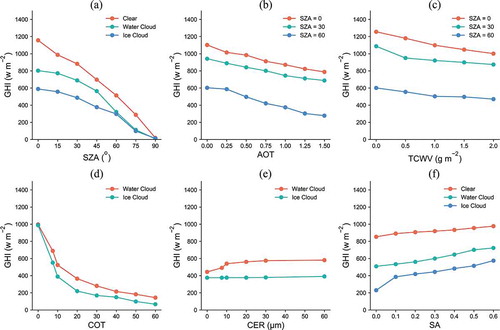
Sensitivity tests shown in Figure 4 are simulated by SBDART, to quantity the uncertainties of the input parameters. U.S. standard atmosphere and rural type aerosol model for clear sky are default settings. More detailed settings are shown in the figure. (Figure 4(a)) shows that GHI decreases with an increase in SZA and (Figure 4(d)) reveals GHI drastically decreases with a rising COT ranging from 0 to 30. As GHI decreases, it exhibits a linear relationship with an increasing AOT as shown in (Figure 4(b)), and with an increasing TCWV as shown in the (Figure 4(c)). An increasing CER in (Figure 4(e)) and SA in (Figure 4(f)) both have a positive impact on the increase in GHI.

Figure 4. (a) Sensitivity of GHI to SZA: Clear: AOT = 0.1, SA = 0.1; Water cloud: COT = 10, CER = 8 μm, SA = 0.1; Ice cloud: COT = 10, CER = 32 μm, SA = 0.1; (b) Sensitivity of GHI to AOT: SA = 0.1; (c) Sensitivity of GHI to CTWV: AOT = 0.1, SA = 0.1; (d) Sensitivity of GHI to COT: Water cloud: SZA = 30°, CER = 8 μm, SA = 0.1; Ice cloud: SZA = 30°, CER = 32 μm, SA = 0.1; (e) Sensitivity of GHI to CER: Water cloud: SZA = 30°, COT = 10,SA = 0.1; Ice cloud: SZA = 30°, COT = 10, SA = 0.1 (f). Sensitivity of GHI to SA: Clear: SZA = 30°, AOT = 0.1; Water cloud: COT = 10, CER = 8 μm, Ag = 0.1; Ice cloud: COT = 10, CER = 32 μm

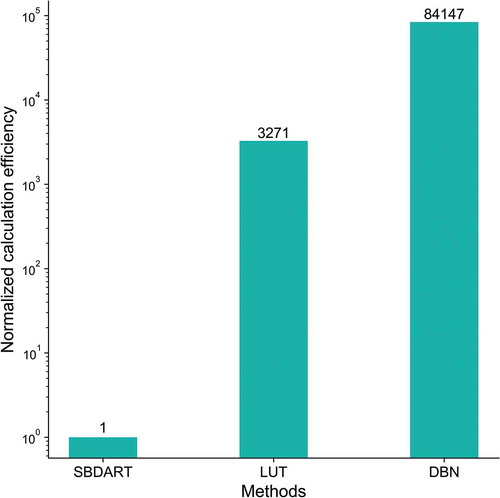
4.2. Evaluation of calculation speed of DBN models

Considering the calculation efficiency of different methods among different methods, Figure 5 shows the difference in calculation speed between SBDART, the LUT method, and the DBN when these run on the same computer platform. There is no doubt that DBN is much faster than the others. Thus, a DBN has significant computation performance advantage to calculate high-speed GHIs when using large satellite data sets.

Figure 5. Comparison of the normalized calculation efficiency of different methods (SBDART results is set as a baseline. Xeon (R) E5-2640 processor and RAM 16 GB)

4.3. Mapping of GHI

Figures 6 and 7 illustrate the instantaneous spatial variations of GHI values over Mainland China with a spatial resolution of 0.05° × 0.05°. Figure 6 and Figure 8 show that GHI is strongly affected by clouds. Note that Figures 6, 7 and 8 have the same indication of date but different of time: Figures 6 and 8 show the 03:00 UTC, and Figure 7 shows the 06:00 UTC, and (a) to (c) in all three figures indicate 21 August 2025 August, 1 November, and 4 November in 2018, respectively. But the GHI for some regions was missed because AOT retrieval and cloud property retrieval failed. This seems to be due to broken clouds. Also, the cloud property product, offered by JAXA, is missed in some regions. Generally speaking, GHI in summer is higher than in winter under cloudless conditions. Tibet, northwestern China and Inner Mongolia possess an abundant solar energy potential due to the lack of cloud cover.

Figure 6. Estimated GHI (w m⁻²) at 03:00 UTC on chosen days: (a) 21 August 2018; (b) 25 August 2018; (c) 1 November 2018; (d) 4 November 2018

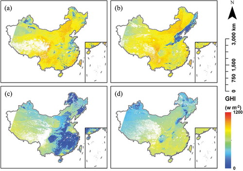
Figure 7. Estimated GHI (w m⁻²) at 06:00 UTC on chosen days: (a) 21 August 2018; (b) 25 August 2018; (c) 1 November 2018; (d) 4 November 2018

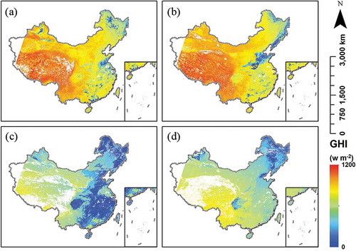
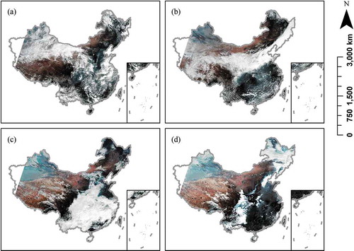
Figure 8. Real colour images from Himawari-8 at 03:00 UTC on chosen days: (a) 21 August 2018; (b) 25 August 2018; (c) 1 November 2018; (d) 4 November 2018

4.4. Validation of GHI

GHI measured at CERN sites were collected in order to compare the accuracy of our proposed method with previous studies. These sites only provided hourly GHI records while the time gap of DBN-GHI results is 10 min. So, ground observations and estimation datasets need to be matched. Thus, the satellite estimates of GHI were averaged from pixels that fall within an approximate radius of 3 pixels from the chosen CERN locations and within 60 minutes of the time recorded by CERN.

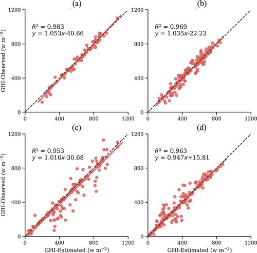
The output of DBN-GHI is validated using the Mean-Absolute-Error (MAE), Normalized-Mean-Absolute-Error (NMAE), Root-Mean-Square-Error (RMSE). MAE measures the overall bias. RMSE quantifies the spread in the distribution of errors. Concerning the NMAE, the normalization is done to compare the relative bias on different days. The statistical parameters are given in Table 3. Figure 9 shows a scatter plot of GHI between Himawari-8 estimate and CERN observations. The subfigures of Figure 9, (a) to (d) illustrate the situations under different conditions: (a) No cloud in summer; (b) No cloud in winter; (c) Have cloud in summer; (d) Have cloud in winter.

Table 3. Summary statistics of the validation results

	Clear sky			Cloudy sky			All sky
	MAE (w m^−2)	NMAE (%)	RMSE (w m^−2)	MAE (w m^−2)	NMAE (%)	RMSE (w m^−2)	MAE (w m^−2)	NMAE (%)	RMSE (w m^−2)
Summer case	27.61	4.61	33.90	45.38	10.68	87.42	45.00	8.02	73.52
Winter case	34.48	7.09	45.60	37.16	9.73	60.88	35.98	8.73	54.68

Figure 9. Validation results at the chosen CERN sites over China: summer clear case is on upper left; winter clear case is on upper right; summer cloud case is located on bottom left; winter cloud case is located on bottom right. (a) If cloud = No & Season = Summer; (b) If cloud = No & Season = Winter; (c) If cloud = Yes & Season = Summer; (d) If cloud = Yes & Season = Winter. Note that subfigures (a) and (b) share the same y-axis lables, as well as (c) and (d). And (a) and (c), (b) and (d) share the same x-axis labels respectively

Zhang et al. (2018) evaluated half-hour averaged GHI over US based on GEOS-13 Geostationary satellite and a lookup table approach. The results demonstrated that overall RMSE were 99.5 w m⁻², 80.0 w m⁻², 127.6 w m⁻², for all-sky, clear-sky, and cloudy-sky, respectively. Damiani et al. (2018) evaluated the Himawari-8 GHI product AMTERASS using observations recorded at four SKYNET stations in Japan. They noted that the agreement with ground-based observations depends on time step used in the validation exercises. A worse agreement was found when smaller time steps were used. In their paper, the RMSE of hourly GHI was usually around 80 w m⁻² on all-sky days. However, there is little research about the assessment of satellite-based hourly surface solar irradiance across China. Shi et al. (2018) evaluated daily and monthly satellite-based GHI products in China. Yu, Wang, and Shi (2018) did similar research in Tibet. Both of them aggregate original satellite GHI products at 10 minutes intervals on daily or monthly scales, to be consistent with daily or monthly ground-based observations.

Overall, the analysis showed that the DBN-GHI estimation match observations at chosen CERN stations well. For all cases, the Pearson correlation coefficient (r) which is the covariance of the two variables divided by the product of their standard deviations (Benesty et al. 2009) ranges from 0.95 to 0.98. The accuracy of values calculated by DBN on clear-sky days is better than that on cloudy days, as shown by a smaller MAE, NMAE and RMSE on clear-sky days and is in agreement with other researchers, e.g. (Shi et al. 2018). The bias under cloudy conditions especial in summer may be influenced by the retrieval accuracy of cloud microphysical parameters (such as COT, CER). Because more water vapour is available during the summer for cloud fabrication causes uncertainties of cloud retrieval. Therefore, the accuracy under summer cloudy condition is worse than that in winter. The obvious difference between winter clear day and summer clear day does not exist. Table 3 demonstrates that RMSE of GHI are around 40 w m⁻² and on clear days. On cloudy days, RMSE are in the range of 60 w m⁻² to 80 w m⁻². RMSE on all-sky day 73 w m⁻² and 54 w m⁻² on summer case and winter case, respectively.

5. Conclusions and further work

We evaluated the performance of DBN-GHI estimates at hourly scale. The results showed that our method could effectively estimate instantaneous GHI with r of larger than 0.95, and an overall RMSE between 30 w m⁻² to 80 w m⁻². The model performs better under clear sky conditions than under cloudy condition. The AOT product, which was derived based on red-blue surface reflectance ratio algorithm, is more reliable. It has a positive impact on decreasing the estimated uncertainty stemming from aerosols.

A large uncertainty may occur due to the quality of cloud property products and the use of the homogeneous one-layer atmosphere assumption. Additionally, the main limitations are cloud attenuation, terrain shading, and over mountainous areas and their combined effect on diffuse and direct radiation (Zhang et al. 2019). Our research ignored the effect caused by terrain shading. To summarize, our proposed new method demonstrates a good potential for accurately estimating instantaneous GHI and conducting research on solar energy potential in flat regions. The applicability of this model for use in mountainous areas need to be improved as the next step.

Acknowledgements

This work was supported by Queen Mary University of London and the China Scholarship Council (CSC).

Further, the first author, Weipeng Xing, has gotten his master’s degree in the University of Chinese Academy of Sciences in 2019, and now he is an academic in Shenzhen Urban Public Safety and Technology Institute (SZSTI).

Disclosure statement

No potential conflict of interest was reported by the authors.

Additional information

Funding

This work was supported by Queen Mary University of London; the China Scholarship Council.

References

- Antonanzas-Torres, F., R. Urraca, J. Polo, and O. Perpiñán-Lamigueiro; R %J Renewable Escobar, and Sustainable Energy Reviews. 2019. “Clear Sky Solar Irradiance Models: A Review of Seventy Models.” Renewable and Sustainable Energy Reviews 107: 374–387. doi:10.1016/j.rser.2019.02.032.
- Benesty, J., J. Chen, Y. Huang, and I. Cohen. 2009. “Pearson Correlation Coefficient.” In Noise Reduction in Speech Processing, 1–4. Springer, Berlin, Heidelberg. https://doi.org/10.1007/978-3-642-00296-0_5
- Berk, A., L. S. Bernstein, and D. C. Robertson. 1987. “MODTRAN: A Moderate Resolution Model for LOWTRAN.” Technical report, 12 May 1986-11 May 1987. United States.
- Beyer, H. G., C. Costanzo, and D. Heinemann. 1996. “Modifications of the Heliosat Procedure for Irradiance Estimates from Satellite Images.” Solar Energy 56 (3): 207–212. doi:10.1016/0038-092X(95)00092-6.
- “CERA-SAT.” Accessed 14 June 2019. https://www.ecmwf.int/en/forecasts/datasets/reanalysis-datasets/cera-sat
- “Chinese Ecosystem Research Network.” Accessed 14 June 2019. http://www.cnern.org.cn/
- Damiani, A., H. Irie, T. Horio, T. Takamura, P. Khatri, H. Takenaka, T. Nagao, T. Y. Nakajima, and R. R. Cordero. 2018. “Evaluation of Himawari-8 Surface Downwelling Solar Radiation by Ground-based Measurements.” Atmospheric Measurement Techniques 11 (4): 2501–2521.
- Deneke, H. M., A. J. Feijt, and R. A. Roebeling. 2008. “Estimating Surface Solar Irradiance from METEOSAT SEVIRI-derived Cloud Properties.” Remote Sensing of Environment 112 (6): 3131–3141. doi:10.1016/j.rse.2008.03.012.
- Fu, B., S. Li, X. Yu, P. Yang, G. Yu, R. Feng, and X. Zhuang. 2010. “Chinese Ecosystem Research Network: Progress and Perspectives.” Ecological Complexity 7 (2): 225–233. doi:10.1016/j.ecocom.2010.02.007.
- Gueymard, C. A., V. Lara-Fanego, M. Sengupta, and Y. Xie. 2019. “Surface Albedo and Reflectance: Review of Definitions, Angular and Spectral Effects, and Intercomparison of Major Data Sources in Support of Advanced Solar Irradiance Modeling over the Americas.” Solar Energy 182: 194–212. doi:10.1016/j.solener.2019.02.040.
- Hinton, G. E. 2002. “Training Products of Experts by Minimizing Contrastive Divergence.” Neural Computation 14 (8): 1771–1800. doi:10.1162/089976602760128018.
- Hinton, G. E. 2007. “Learning Multiple Layers of Representation.” Trends in Cognitive Sciences 11 (10): 428–434. doi:10.1016/j.tics.2007.09.004.
- Hinton, G. E. 2012. A Practical Guide to Training Restricted Boltzmann Machines. In: Montavon G., Orr G.B., Müller KR. (eds) Neural Networks: Tricks of the Trade. Lecture Notes in Computer Science, vol 7700. Springer, Berlin, Heidelberg. https://doi.org/10.1007/978-3-642-35289-8_32.
- Hinton, G. E., and S. Osindero, Yee-Whye %J Neural computation Teh. 2006. “A Fast Learning Algorithm for Deep Belief Nets.” Neural Computation 18 (7): 1527–1554.10.1162/neco.2006.18.7.1527.
- “Japan Aerospace Exploration Agency.” Accessed 14 June 2019. https://www.eorc.jaxa.jp/ptree/
- Key, J. R., and A. J. Schweiger. 1998. “Tools for Atmospheric Radiative Transfer: Streamer and FluxNet.” Computers & Geosciences 24 (5): 443–451. doi:10.1016/S0098-3004(97)00130-1.
- Keyvanrad, M. A., and M. M. Homayounpour. 2014. “A Brief Survey on Deep Belief Networks and Introducing A New Object Oriented Toolbox (Deebnet).” arXiv Preprint arXiv:1408.3264.
- Kosmopoulos, P. G., S. Kazadzis, M. Taylor, P. I. Raptis, I. Keramitsoglou, C. Kiranoudis, and A. F. Bais. 2018. “Assessment of Surface Solar Irradiance Derived from Real-time Modelling Techniques and Verification with Ground-based Measurements.” Atmospheric Measurement Techniques 11 (2): 907–924. doi:10.5194/amt-11-907-2018.
- Li, X., F. Wagner, W. Peng, J. Yang, and D. L. Mauzerall. 2017. “Reduction of Solar Photovoltaic Resources Due to Air Pollution in China.” Proceedings of the National Academy of Sciences 114 (45): 11867–11872. doi:10.1073/pnas.1711462114.
- Lin, C., K. Yang, J. Huang, W. Tang, J. Qin, X. Niu, Y. Chen, D. Chen, N. Lu, and R. Fu. 2015. “Impacts of Wind Stilling on Solar Radiation Variability in China.” Scientific Reports 5 (1): 15135. doi:10.1038/srep15135.
- Maxwell, E., S. Wilcox, and M. Rymes. 1993. “Users Manual for Seri Qc Software, Assessing the Quality of Solar Radiation Data.” Solar Energy Research Institute, Golden, CO http://www.osti.gov/bridge
- Mayer, B., and A. Kylling. 2005. “The libRadtran Software Package for Radiative Transfer Calculations-description and Examples of Use.” Atmospheric Chemistry and Physics 5 (7): 1855–1877. doi:10.5194/acp-5-1855-2005.
- “The Moderate Resolution Imaging Spectroradiometer (MODIS).” Accessed 14 June 2019. https://lpdaac.usgs.gov/products/mcd43a3v006/
- Nakajima, T., and M. Tanaka. 1986. “Matrix Formulations for the Transfer of Solar Radiation in a Plane-parallel Scattering Atmosphere.” Journal of Quantitative Spectroscopy and Radiative Transfer 35 (1): 13–21. doi:10.1016/0022-4073(86)90088-9.
- Perez, R., R. Seals, and A. Zelenka. 1997. “Comparing Satellite Remote Sensing and Ground Network Measurements for the Production of Site/time Specific Irradiance Data.” Solar Energy 60 (2): 89–96. doi:10.1016/S0038-092X(96)00162-4.
- Pinker, R. T., R. Frouin, and Z. Li. 1995. “A Review of Satellite Methods to Derive Surface Shortwave Irradiance.” Remote Sensing of Environment 51 (1): 108–124. doi:10.1016/0034-4257(94)00069-Y.
- Ricchiazzi, P., S. Yang, C. Gautier, and D. Sowle. 1998. “SBDART: A Research and Teaching Software Tool for Plane-parallel Radiative Transfer in the Earth’s Atmosphere.” Bulletin of the American Meteorological Society 79 (10): 2101–2114. doi:10.1175/1520-0477(1998)079<2101:SARATS>2.0.CO;2.
- Rumelhart, D. E., G. E. Hinton, and R. J. Williams. 1988. “Learning Representations by Back-propagating Errors.” Cognitive Modeling 5 (3): 1.
- Schmidhuber, J. 2015. “Deep Learning in Neural Networks: An Overview.” Neural Networks 61: 85–117.
- Shi, H., W. Li, X. Fan, J. Zhang, B. Hu, L. Husi, H. Shang, X. Han, Z. Song, and Y. Zhang. 2018. “First Assessment of Surface Solar Irradiance Derived from Himawari-8 across China.” Solar Energy 174: 164–170. doi:10.1016/j.solener.2018.09.015.
- “SRTM: NASA Shuttle Radar Topography Mission.” Accessed 14 June 2016. http://vterrain.org/Elevation/SRTM/
- Takenaka, H., T. Y. Nakajima, A. Higurashi, A. Higuchi, T. Takamura, R. T. Pinker, and T. Nakajima. 2011. “Estimation of Solar Radiation Using a Neural Network Based on Radiative Transfer.” Journal of Geophysical Research: Atmospheres 116 (D8): D8. doi:10.1029/2009JD013337.
- Taylor, M., P. G. Kosmopoulos, S. Kazadzis, I. Keramitsoglou, and C. T. Kiranoudis. 2016. “Neural Network Radiative Transfer Solvers for the Generation of High Resolution Solar Irradiance Spectra Parameterized by Cloud and Aerosol Parameters.” Journal of Quantitative Spectroscopy and Radiative Transfer 168: 176–192. doi:10.1016/j.jqsrt.2015.08.018.
- Xiaojun, N. I. U., T. A. N. G. Jiakui, Z. H. A. N. G. Zili, C. U. I. Linli, X. I. N. G. Weipeng, and S. O. N. G. Yi. 2019. “The Method of Aerosol Retrieval Using Himawari-8 Satellite Data and Its Application in Monitoring Haze Process.” Journal of University of Chinese Academy of Sciences 36 (5): 671–681. doi:10.7523/j.2095-6134.2019.05.013.
- Xie, Y., M. Sengupta, and J. Dudhia. 2016. “A Fast All-sky Radiation Model for Solar Applications (FARMS): Algorithm and Performance Evaluation.” Solar Energy 135: 435–445. doi:10.1016/j.solener.2016.06.003.
- Yu, Y., T. Wang, and J. Shi. 2018. “Assessment of Two Satellite-Based Land Surface Shortwave Downward Radiation Datasets over the Tibetan Plateau.” Paper presented at the IGARSS 2018–2018 IEEE International Geoscience and Remote Sensing Symposium, Valencia, 2018, pp. 1180-1182, doi: 10.1109/IGARSS.2018.8519578.
- Zarzalejo, L. F., L. Ramirez, and J. Polo. 2005. “Artificial Intelligence Techniques Applied to Hourly Global Irradiance Estimation from Satellite-derived Cloud Index.” Energy 30 (9): 1685–1697. doi:10.1016/j.energy.2004.04.047.
- Zhang, H., C. Huang, S. Yu, L. Li, X. Xin, and Q. Liu. 2018. “A Lookup-table-based Approach to Estimating Surface Solar Irradiance from Geostationary and Polar-orbiting Satellite Data.” Remote Sensing 10 (3): 411. doi:10.3390/rs10030411.
- Zhang, S., X. Li, J. She, and X. Peng. 2019. “Assimilating Remote Sensing Data into GIS-based All Sky Solar Radiation Modeling for Mountain Terrain.” Remote Sensing of Environment 231: 111239. doi:10.1016/j.rse.2019.111239.