VEdge_Detector: automated coastal vegetation edge detection using a convolutional neural network

ABSTRACT

Coastal communities, land covers, and intertidal habitats are vulnerable receptors of erosion, flooding or both in combination. This vulnerability is likely to increase with sea level rise and greater storminess over future decadal-scale time periods. The accurate, rapid, and wide-scale determination of shoreline position, and its migration, is therefore imperative for future coastal risk adaptation and management. This paper develops and applies an automated tool, VEdge_Detector, to extract the coastal vegetation line from high spatial resolution (Planet’s 3 to 5 m) remote-sensing imagery, training a very deep convolutional neural network (holistically nested edge detection), to predict sequential vegetation line locations on annual to decadal timescales. Red, green, and near-infrared (RG-NIR) was found to be the optimum image spectral band combination during neural network training and validation. The VEdge_Detector outputs were compared with vegetation lines derived from ground-referenced positional measurements and manually digitized aerial photographs, which were used to ascertain a mean distance error of <6 m (two image pixels) and >84% producer accuracy (P_A) at six out of the seven sites. Extracting vegetation lines from Planet imagery of the rapidly retreating cliffed coastline at Covehithe, Suffolk, United Kingdom, has identified a landward retreat rate >3 m year⁻¹ (2010–2020). Plausible vegetation lines were successfully retrieved from images in The Netherlands and Australia, which were not used to train the neural network, although significant areas of exposed rocky coastline proved to be less well recovered by VEdge_Detector. The method therefore promises the possibility of generalizing to estimate retreat of sandy coastlines from Planet imagery in otherwise data-poor areas, which lack ground-referenced measurements. Vegetation line outputs derived from VEdge_Detector are produced rapidly and efficiently compared to more traditional non-automated methods. These outputs also have the potential to inform upon a range of future coastal risk management decisions, incorporating future shoreline change.

1. Introduction

Coastal zones are often characterized by high human population densities, presence of critical infrastructure, and internationally designated sites of nature conservation significance. In the United Kingdom (UK) alone, damage caused by coastal flooding and erosion frequently exceeds £260 million per year, with the number of properties vulnerable to coastal erosion projected to increase from 9,800 to greater than 100,000 by 2080 (Committee on Climate Change 2018). Detecting contemporary shoreline position and likely rates of future change is vital for understanding coastal morphological response to changing marine climates and subsequent landscape recovery, and the way these dynamics impact upon human lives and livelihoods. This information is necessary to better inform coastal risk management decisions, including the suitability (or lack thereof) of projected human interventions in the coastal zone (De Andrés, Barragán, and Scherer 2018).

Shoreline detection techniques can be broadly categorized into datum-based or proxy-based methods (Pollard, Brooks, and Spencer 2019a). Datum-based methods use light detection and ranging (lidar) or other elevation capture methods (e.g. terrestrial laser scanning) to generate digital terrain models (DTMs) from which the shoreline can be extracted (Brock and Purkis 2009). From these DTMs, shorelines are commonly delineated as the mean high water (MHW) or other water elevation contour (Moore, Ruggiero, and List 2006). Datum-based methods determine both shoreline position and the 3D profile of the coastal zone, but infrequent image capture and inconsistent spatial coverage limit widespread applications (Pardo-Pascual et al. 2018).

Proxy-based shoreline analysis can be broadly classified by the use of geomorphological, vegetation, water or human features (Toure et al. 2019), with detection of visibly discernible features through multispectral or panchromatic optical image analysis. The instantaneous waterline position is the dominant shoreline proxy extracted from optical remote-sensing imagery (Boak and Turner 2005). It is commonly delineated by thresholding the normalized difference water index (NDWI) of a coastal multispectral image (McFeeters 1996; Hagenaars et al. 2018) or by conducting land cover classification (Pekel et al. 2016). Using these methods, global, decadal-scale changes in waterline position have been calculated to determine large-scale trends in shoreline position (Luijendijk et al. 2018; Mentaschi et al. 2018). However, collating a time-series of instantaneous waterline position in isolation does not necessarily provide an indication of net shoreline migration. The amplitude of horizontal change in waterline position caused by diurnal or semi-diurnal tidal cycles can vary depending on beach gradient, which in turn is often linked to beach sediment size and sorting. So depending on where in the tidal frame the image was captured, tidal range potentially has a greater effect on waterline position than decadal shoreline accretion or erosion (Pugh and Woodworth 2014). This issue can be mitigated by calculating the mean waterline position extracted from multiple, temporally adjacent, images (Almonacid-Caballer et al. 2016) but this removes the ability to detect short-term variability and, even then, there are spring-neap, equinoctical and nodal tide cycles operating at different timescales. Waterline position can be tidally corrected by considering slope profile and tidal stage during image capture (Vos et al. 2019); although approximate slope profiles have to be used when concurrent datum-based measurements are not available. Thus, given the difficulties of deriving a robust waterline position indicator, there is potential value in seeking out alternative shoreline proxies from remote-sensing imagery to quantify temporal rates of shoreline change.

The vegetation line is a shoreline proxy which can be flood-responsive, representing the limits to spring high tide flooding, or erosion-responsive, delineating the boundary between the upper beach and the base of sand dunes or soft rock cliffs (Pollard, Spencer, and Brooks 2019b; Toure et al. 2019). Coastal vegetation lines have been derived through manual digitization (e.g. Ferreira et al. 2006; Theiler et al., 2013), or by semi-automated methods including thresholding the normalized difference vegetation index (NDVI, Rahman et al., 2011) and supervised classification of coastal land covers (Zarillo, Kelley, and Larson 2008). However, fully automated vegetation line extraction using thresholding and image classification is precluded by variability in the spectral properties of vegetation due to phenology, species, biomass density, vegetation line boundary abruptness, time of year, and azimuth. Manual selection of threshold values or class numbers can be time consuming and optimal values can vary within one image. Due to these difficulties, there is a need to investigate the ability of alternative, fully automated methods to extract the vegetation line.

Other automated methods used to detect edges in remote-sensing imagery can be separated into grey-scale or multispectral edge detectors. Grey-scale edge detection methods include well-established kernel-based methods, including Sobel, Laplacian, and Canny edge detection. These single-sized kernels have been used to delimit coastal waterlines as locations with the greatest rate of change in greyscale intensity (Pardo-Pascual et al. 2012; Luijendijk et al. 2018). These methods, however, lose valuable spectral information when converting multispectral imagery to a single band, and they lack the inclusion of semantic information, meaning they may also detect irrelevant boundaries, such as field edges and roads.

Machine learning tools, including support vector machines (SVM) and random forests (RF), have been used to classify land covers in multispectral imagery to assist shoreline detection. SVMs maximize the distance between pixels assigned to different classes in feature space (Elnabwy et al. 2020). The coastal waterline has been identified as the boundary between pixels classified by the SVM tool as land or water (Zhang, Jiang, and Xu 2013; Elnabwy et al. 2020). Choung and Jo (2017) found the mean error in waterline position to be lower using SVM compared to NDWI thresholding, but SVM outputs contained a lot of ‘speckle’, attributable to the similar spectral properties of shallow water, sand, and rock surfaces.

RF methods use decision trees to split pixels into subsets with increasingly homogenous pixel values (Breiman 2001). Typically, an ensemble of trees are used, with each individual tree trained using a different sample of the original data set of pixels. Within each tree, some pixels are withheld during training and subsequently used to validate the accuracy of the classification method (Breiman 2001). Binary land and water maps have been generated using RF (Bayram et al. 2017; Demir et al. 2017) although large mean errors (>22 m) have been recorded between manually digitized shorelines and RF derived shorelines. These differences can be attributed to noise contained within the pansharpened images (Demir et al. 2017). Further, the shallow nature of RF and SVM means they are not robust to identifying spectral–spatial relationships, most saliently that adjacent pixels are likely to belong to the same feature class (Zhang, Zhang, and Du 2016). No applications of RF or SVM to detect the coastal vegetation line could be found in the literature; RF and SVM have only been used to detect the waterline from imagery pertaining to a localized area of interest. Further analysis is necessary to determine whether SVM and RF models, which do not consider the value of neighbouring pixels when classifying a pixel, can be generalized, so as to detect waterline position in other global locations.

More recently, convolutional neural networks (CNN) have received increased attention as a way to effectively detect edges in remote-sensing imagery. This is in part because they simultaneously consider the value of the pixel of interest and neighbouring pixels (Kokkinos, 2015; Zhang, Zhang, and Du 2016). CNNs convolve kernels of different sizes over the raw input image. Smaller kernels (e.g. 3 × 3) capture detailed edge structures but suffer from high incidence of false positives (noise). Conversely, larger kernels detect only the most salient edges, generating blurred boundaries and missing localized detail. Optimal fusing of the outputs from different sized kernels subsequently identifies the most likely location of true edges and minimizes noise by considering that edges will be in the same location irrespective of kernel size (Ren 2008).

Holistically nested edge detection (HED) is an example of a CNN which progressively reduces image resolution, instead of increasing kernel size, to achieve multi-scale image convolution (Xie and Tu 2015). The HED model architecture contains five separate sets of convolutional layers, all using 3 × 3 kernels, which are each separated by 2 × 2 max pooling layers to reduce image resolution. A side output layer is produced after every set of convolutional layers. The first side output contains local boundary detail but is susceptible to noise and false inland boundaries. Conversely, side output 5 only detects salient boundaries and is robust to image noise, but the predicted coastal vegetation edge is blurred. These five side output layers are optimally fused to derive the final output, predicting the likelihood of each pixel being an edge (Xie and Tu 2015; see Figure 1 for a graphical overview of HED architecture).

Figure 1. Holistically nested edge detection (HED) architecture. Three spectral bands from every satellite image are selected as HED input. Input images are fed through five distinct stages of image convolution, and between each stage, a max pooling layer decreases image size. The squares to the bottom left of the image detail the number of convolution kernels at each stage. The side outputs are resized and optimally fused to generate the output.

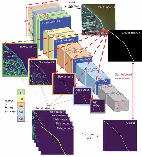
During HED training, every epoch contains a feed- forward and backpropagation stage. During the feed-forward stage, the internal weights in the HED model are used to derive the predicted edge locations from the raw input image. The difference, or loss, between the predicted vegetation line position and the ground-truth binary image is back-propagated through the hidden layers of the HED model, to update the internal HED model weights. These updated weights are subsequently used in the feed-forward stage of the next epoch of HED training (see Xie and Tu (2015) and Kokkinos (2015) for a full summary of HED architecture and functionality).

Applications of CNN methods, including HED, to detect edges have recently increased in number, due to enhanced computer processing power and greater image availability to train CNNs, e.g. natural image data sets including the Berkeley segmentation data set (Arbelaez et al. 2007) and ImageNet (Stanford Vision Lab 2016). The Visual Geometry Group Network (VGGNet-16) model is a CNN with a very similar architecture to HED but contains no side outputs. The model was trained using the ImageNet data set to detect all objects in natural Red Green Blue (RGB) images, e.g. images of animals, humans and everyday items (Simonyan and Zisserman 2014). Applications of HED to detect every object in natural images are widespread, but remote-sensing applications, where images contain more noise and a higher density of boundaries, remain highly limited. A key research gap is the retraining and fine-tuning of these generalist edge detection CNNs to be able to differentiate between separate types of edge in remote-sensing imagery and exclusively extract edges of interest.

To exclusively detect particular types of edge in remote-sensing imagery, some studies have updated or fine-tuned the weights within pre-existing CNNs by retraining them with remote-sensing image pairs. Richer convolutional networks (RCF), which are CNNs with a similar architecture to HED, have been fine-tuned to exclusively detect building boundaries in remote-sensing imagery, achieving a higher accuracy than other generalist edge detection algorithms (Lu et al. 2018). Fine tuning was conducted by training the RCF on 1856 image pairs containing an urban scene and a binary image showing building edge and non-edge locations (Lu et al. 2018). Similarly, a U-Net neural network was retrained with Landsat imagery to predict glacial calving front locations (Mohajerani et al. 2019). Remote-sensing applications of HED, or modified versions, have been used to detect field boundaries (H. Liu et al., 2019) and to derive land cover classification (Marmanis et al. 2018). X.Y. Liu et al. (2019) modified the standard convolution structure of HED to detect shorelines in heavily urbanized Jiaozhou Bay, China. HED was reported to outperform Sobel and Canny Edge Detection (producer accuracy (P_A): Sobel = 0.66, Canny = 0.82, modified HED = 0.95) but no information was provided on the shoreline proxy used. Furthermore, this study trained HED using exclusively RGB spectral bands; further analysis is necessary to identify the optimum spectral band combination during HED training. These abovementioned studies highlight the potential of retraining a CNN to fine-tune its internal weights to exclusively detect a particular type of edge in remote-sensing imagery. To date, this approach has not been applied to exclusively detect coastal vegetation edges from remote sensing imagery.

This study aims to train and apply a holistically nested edge detection (HED) model to extract coastal vegetation lines. The objectives of the paper are to (i) train a HED model using coastal remote-sensing imagery, namely Planet 3 m and 5 m resolution imagery (PlanetScope and RapidEye); (ii) assess the performance of HED in extracting the coastal vegetation line when trained using different combinations of spectral bands as input across a range of coastal settings (Winterton, Suffolk, UK; Perranuthnoe, Cornwall, UK; Bribie Island, Australia and Wilk-Ann-Zee, The Netherlands); (iii) compare Vedge_Detector performance against other experimental methods previously used to detect the coastal vegetation edge, namely ground-referenced measurements and manual digitization of remote sensing and aerial imagery; and (iv) incorporate the best performing HED model within VEdge_Detector to detect shoreline change from sequential images of Covehithe, Suffolk, UK, between 2010 and 2020.

2. Materials and methods

2.1. Remote-sensing imagery data sources

A total of 78 Planet images (PlanetScope and RapidEye, with 3 and 5m spatial resolution respectively) were selected for HED training (Planet Team 2017). Ortho Scene product level imagery was chosen, meaning Planet had orthorectified and radiometrically corrected images prior to image download. Locations were chosen to encompass a diverse range of geomorphic landforms, tidal ranges and vegetation types (see the supplemental material). Training image sizes ranged from 6.3 km² to 1557.5 km² and images were selected from all years when Planet imagery was available (2010 to 2020). Multiple images were collected from each location to ensure the training data set contained scenes captured at different tidal stages. This ensured multiple images of the same shoreline, with different beach widths, were contained in the training data set.

2.2. Holistically nested edge detection (HED) training

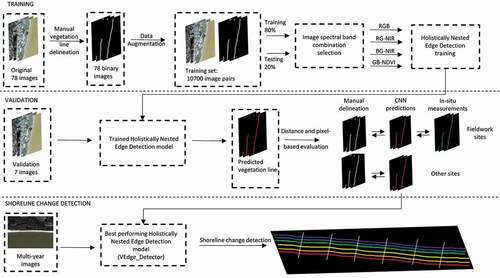
All steps taken in this study were separated into three stages: HED training using coastal remote-sensing imagery; validation of the trained HED models; and digital shoreline change analysis using the best performing HED model. The training and validation stages determined the optimal combination of remote-sensing spectral bands to train the HED model, while keeping the HED model architecture constant. The best performing HED model became the VEdge_Detector tool, developed to extract vegetation lines in the shoreline change stage. Figure 2 provides a graphical overview of the three analytical stages.

Figure 2. Overview of the three stages carried out in this study. Four holistically nested edge detection (HED) models were independently trained using different spectral band combinations (training). The performance of each HED model was evaluated using a separate image set (validation). The best performing HED model, trained on images with spectral band combination red, green, near-infrared (RG-NIR), formed the VEdge_Detector tool. This tool detected the vegetation line position from multiple images of the same shoreline captured over a 10-year period (shoreline change detection).

2.2.1. Manual digitization of the vegetation line

To generate the training data set, vegetation lines were manually digitized from all 78 training images in ArcGIS 10.5.1. The image NDVI was overlaid at 70% transparency to aid visual vegetation line identification. Where vegetation lines were interrupted, the seaward extent of inland waterbodies or urban areas were used. Vegetation line shapefiles were converted into binary raster edge maps (binary images), with edge pixel values set to 1 and non-edge pixels to 0. Image pairs were subsequently established, containing the original image and the binary image.

2.2.2. Data Augmentation

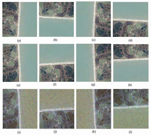
A large number of images are required during HED training to refine the internal weights within the HED model. Manual digitization of this number of images would be too time consuming; therefore, data augmentation was used to substantially increase training data size from 78 to 10,700 image pairs. Larger images were cropped to size 480 × 480 pixels (the default image size used by the HED architecture) at multiple locations. The uncropped larger images also formed part of the training data set, but were resized to 480 × 480 pixels prior to HED training. Image pairs were flipped vertically, rotated by 90, 180, and 270 degrees and subject to the introduction of Gaussian noise (Figure 3). Gaussian noise was not added to the binary images. Images were rotated around five different points of origin. Image pairs not containing any vegetation line after rotation were automatically discarded. All image pairs were shuffled and randomly assigned into training (80%) and testing (20%) sets prior to HED input. The proportion of land cover in each image varied from 2% to 98%.

Figure 3. Transformations used in data augmentation (a) original image (cropped to 480 × 480 pixel size), (b) – (d) original image rotated by 90°, 180°, and 270°, (e) original image flipped vertically, (f)–(h) flipped image rotated by 90°, 180°, and 270°, (i)–(l) Gaussian noise added to the flipped images. Transformations (b)–(h) were simultaneously conducted on the binary images.

2.2.3. Holistically nested edge detection (HED) training

HED training was conducted to modify the model’s internal weights to increase the model’s ability to exclusively detect coastal vegetation edges. To speed up HED training, non-zero weights were initialized prior to training commencement. This study initialized the internal weights contained within the VGGNet-16 architecture prior to training. The weights contained within the VGGNet-16 architecture were derived from training the model on 1.2 million natural images to detect everyday objects, e.g. animals, people and urban features. Using the weights contained within the VGGNet-16 architecture increased the speed of HED training compared to using randomly assigned weights. The key difference between the architecture in VGGNet-16 and HED is that HED contains side outputs. The side outputs enable deep supervision, whereby every side output is directly compared to the binary image to calculate loss. By comparison, in VGGNet-16 only the final output is compared to the binary image. Deep supervision guides the neural network to detect transparent objects, i.e. to only detect the edges of objects at a per-pixel level rather than the entirety of an object (Xie and Tu 2015).

To substantiate the assertion that the default weights in the VGGNet-16 architecture were not suitable for detecting exclusively coastal vegetation edges, a HED model containing the default VGGNet-16 weights was used to predict the coastal vegetation edge in an image of Winterton, Suffolk, UK. This HED model failed to detect the coastal vegetation line and instead detected the waterline and other inland boundaries (e.g. roads and field edges). This was attributed to the weights in the VGGNet-16 architecture originally being trained to classify all objects in a natural RGB image, whereas the objective of this study is to exclusively extract the vegetation line in remote-sensing imagery and discard other boundaries. This reinforced the necessity to retrain the HED model to refine the model weights, using the image pairs derived through manual digitization and data augmentation.

During every epoch of HED training, the internal weights in the HED model were used to predict the coastal vegetation line position from the raw image. The class-balanced cross entropy loss function was used to calculate the difference, or loss, between the predicted vegetation line position and the binary image. The loss function was class-balanced to account for the large imbalance between edge and non-edge pixels, i.e. the vast majority of pixels in every image were non-edge. To prevent the HED model from achieving very accurate results if it predicted all pixels to be non-edge, a scaling factor was used. This was calculated by determining the proportion of edge to non-edge pixels in each image. This scaling factor ensured that the HED model was penalized proportionately more for predicting a false negative (predicting an edge pixel to be a non-edge) than a false positive (predicting a non-edge pixel to be an edge).

HED model training was implemented in Python’s Keras library with Tensorflow backend. The code for the training of HED was modified from Liu (2018) to enable input of 16 bit Planet imagery; selection of the desired image band combination; and the calculation of NDVI. The HED model was run in parallel on four Tesla P100-PCIE-16GB GPUs for 1000 epochs, with a running time of seven h 45 min per spectral band combination. The VEdge_Detector tool, instructions, and input image specifications are available from GitHub (github.com/MartinSJRogers).

2.3. Validation

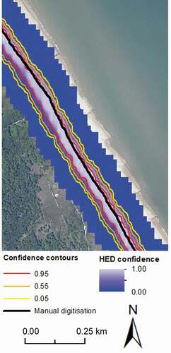
The HED model performance was validated by predicting the vegetation line location in seven images not previously seen by the model. All output prediction pixel values ranged between 0 and 1, representing the range in HED confidence that the pixel represented the vegetation line. Confidence contours were used to determine where ground referenced measurements were located in relation to predicted vegetation line confidence curves. HED outputs were accordingly contoured at 0.1 intervals between 0.05 and 0.95 for subsequent model evaluation through comparison with ground-referenced measurements. All contours had a landward and seaward line (see Figure 4 for a demonstration of the vegetation line contours produced).

Figure 4. Example of 0.05 (yellow), 0.55 (orange), and 0.95 (red) confidence contours produced by VEdge_Detector at Winterton, UK. The confidence contours were generated from the raw VEdge_Detector output, which is overlaid as the blue colour ramp. Light and dark blue pixels represent the locations predicted as being an edge pixel with a high and low confidence, respectively. The manually digitized vegetation line (black) is displayed for visual comparison. Land and sea are found to the left and right of the image, respectively. Aerial imagery, provided by the Environment Agency with 40 cm resolution, is used as a backdrop (Environment Agency, 2020).

Distance and pixel-based evaluation metrics were used to determine the best performing HED model. Distance-based evaluation of HED performance was conducted by comparing (i) HED model prediction contours (confidence contours) with ground-referenced measurements of vegetation line location; (ii) confidence contours to a manually digitized vegetation line of the same image; and (iii) ground-referenced measurements to manual digitization.

The ArcMap plugin Digital Shoreline Analysis System (DSAS; Thieler et al. 2009; USGS 2018) v5.0 was used in ArcGIS 10.5.1 to calculate the distance between shorelines for comparators (i), (ii), and (iii). Distance calculations were made on transects generated at 10 m alongshore intervals, orthogonal to the dominant shoreline orientation. To reduce transect crossing on sinuous coastlines, each transect was drawn orthogonal to a smoothed baseline. This was generated by calculating mean baseline angle over a 200 m interval, with the transect location at the midpoint. Root mean square error (RMSE, Equation (1)(1) $RMSE=\sqrt{\frac{1}{n-1}\sum _{i=1}^n{\left(o_i-p_i\right)}^2}$(1) ) measured the distance between lines. Mean absolute error (MAE, Equation (2)(2) $MAE=\frac{1}{n}\sum _{i=1}^n\left|o_i-p_i\right|$(2) ) determined the net landward (positive) or seaward (negative) bias in prediction contours as shown in the following equations.

(1) $RMSE=\sqrt{\frac{1}{n-1}\sum _{i=1}^n{\left(o_i-p_i\right)}^2}$(1)

(2) $MAE=\frac{1}{n}\sum _{i=1}^n\left|o_i-p_i\right|$(2)

where o and p are observed and predicted vegetation line positions along each transect, i, respectively, and n is the number of transects. MAE values were assigned as negative if the predicted contours were consistently seaward of the line derived from ground-reference measurements or manual digitization.

The pixel-based evaluation metrics used were user accuracy (Equation (3)(3) $U_A=\frac{P_{True}}{P_{True}+P_{False}}$(3) ), producer accuracy (Equation (4(4) $P_A=\frac{P_{True}}{P_{True}+N_{False}}$(4) )), and F₁ (Equation (5)(5) $F_1=\frac{P_A\times U_A}{P_A+U_A}$(5) ). All three metrics are suited to classification tasks with imbalance in class populations (e.g. non-edge pixels constitute >90% of the image),

(3) $U_A=\frac{P_{True}}{P_{True}+P_{False}}$(3)

(4) $P_A=\frac{P_{True}}{P_{True}+N_{False}}$(4)

(5) $F_1=\frac{P_A\times U_A}{P_A+U_A}$(5)

where U_A and P_A are the user accuracy and producer accuracy values, respectively. U_A values are more sensitive to the detection of inland non-coastal boundaries, so are typically lower than P_A values. P_True = True Positive and N_True = True Negative, each corresponding to correctly classified pixels and P_False = False Positives and N_False = False Negative, each corresponding to incorrectly classified pixels. A pixel incorrectly predicted to be the vegetation line will be classified as a false-positive pixel, irrespective of the distance from the manually digitized or ground referenced line. To account for ‘near-misses’, where HED predicts the vegetation line to be at pixels close to the ground-referenced or manual digitization measurements, the manually digitized and ground referenced lines were buffered to be three pixels wide (instead of one). Relaxed U_A, P_A, and F₁ scores were calculated by comparing HED outputs to the buffered ground referenced and manually digitized vegetation line measurements.

2.3.1. Validation image locations

Seven sites were used for HED validation (Table 1). High-resolution ground measurements were collected from three of these seven locations along the Suffolk coastline of eastern England on 7 September 2019 (Walberswick, Dunwich and Covehithe) using a real-time kinematic global positioning system (RTK-GPS) with horizontal positional accuracy of 30 mm. Soft sandy cliffs are located at Covehithe with sharp cliff-top edge vegetation lines. In contrast, a more complex vegetation line on a mixed sand and shingle barrier is present at Walberswick and Dunwich (Pye and Blott 2006). To ensure at least one ground-referenced measurement per pixel, points were captured approximately every 2 m alongshore and whenever there was a notable change in vegetation line direction. At Dunwich and Covehithe, isolated vegetation patches situated in front of the continuous vegetation line were not demarcated. At Walberswick, two vegetation lines were generated from ground-referenced measurements: (i) a landward continuous vegetation line and (ii) locations of isolated seaward vegetation patches. Confidence contours were compared to both vegetation lines derived from ground-referenced measurements at this site.

Table 1. Locations of holistically nested edge detection validation images. Other columns provide information on dominant shoreline direction, spring and neap tidal ranges, dominant sediment type, geomorphology, and climate at each site as well as whether ground-referenced measurements of the coastal vegetation edge were collected

Location	Country	Tidal range (m)	Dominant vegetation type	Geomorphology	Climate	Ground-referenced data collected (Yes/ No)
Walberswick	UK (Suffolk)	2.5(spring)0.5 (neap)	Psammosere dune vegetation	Dune	Temperate	Yes
Covehithe	UK (Suffolk)	2.5 (spring)0.5 (neap)	Cliff top grasses/ agricultural crops.	Soft sandy cliffs	Temperate	Yes
Dunwich	UK (Suffolk)	2.5 (spring)0.5 (neap)	Psammosere dune vegetation	Shingle dune	Temperate	Yes
Winterton	UK (Suffolk)	2.5 (spring)0.5 (neap)	Psammosere dune vegetation	Dune	Temperate	No
Perranuthnoe	UK (Cornwall)	6.0 (spring)2.0 (neap)	Cliff top grasses and Psammosere dune vegetation	Beach dunes and rocky cliff	Temperate	No
Wilk-Ann-See	The Netherlands	4.0 (spring)2.0 (neap)	Psammosere dune vegetation	Dune	Temperate	No
Bribie Island	Queensland, Australia	2.0 (spring)0.5 (neap)	Eucalyptus forest	Barrier island	Sub-tropical	No

Ground-referenced measurements were compared to HED vegetation line predictions generated from a 3 m resolution PlanetScope image, using distance and pixel-based evaluation metrics outlined above. The PlanetScope image was captured on 12 September 2019 and was previously unseen by the HED model. Between 7 and 12 September 2019 waves approached from a dominant north easterly direction and rarely exceeded 1 m significant wave height (maximum peak significant wave height at Southwold Approach was 1.45 m (Cefas 2020)). Due to these wave conditions, there is a high degree of confidence that the vegetation line remained stable over this time period.

The trained HED model was also used to predict the vegetation line position at four additional locations, where ground-referenced measurements were not collected (Table 1). At these locations, HED output prediction contours were compared solely to manually digitized vegetation lines. Images from two locations (Winterton, UK and Perranuthnoe, UK) were used during HED training but different image dates were used (training image dates: 2018 and 2019, testing image dates: 2010 and 2015). The other two locations were previously unseen by the neural network: Wilk-Ann-See, The Netherlands and a separate section of Bribie Island, Australia.

2.4. Determining the optimum spectral band combination

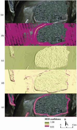
The default VGGNet-16 weights can only be initialized in a HED model which accepts images with three spectral bands. The performance of the HED model was therefore independently trained using four different combinations of three spectral bands: red green near-infrared (RG-NIR), RGB, RB-NIR, and RG-NDVI. Output predictions from the four HED models were compared to select the most appropriate model for vegetation line detection. Figures 5–7 provide a comparison of HED performance using different spectral band combinations at three locations not contained in either the training or validation data set: Cromer, UK; Varela, Guinea-Bissau and Wyk auf Föhr, Germany. The HED models trained on spectral band combinations RG-NDVI and RGB predicted every pixel in the image to be the coastal vegetation edge, these models were therefore rejected. Only the HED models trained on images with spectral band combinations RG-NIR and RB-NIR were able to discard pixels not pertaining to the coastal vegetation edge. The HED model trained on RB-NIR spectral band images was still unable to discard many non-edge pixels and as a result produced very low U_A results of 0.06, 0.02, and 0.02 at Cromer, Varela, and Wyk auf Föhr, respectively. In contrast, the HED model trained using spectral bands RG-NIR was able to predict the location of the coastal vegetation edge with a U_A of 0.26, 0.59 and 0.25 at Cromer, Varela, and Wyk auf Föhr, respectively. The HED model trained using images with RG-NIR spectral bands was thus used to form the basis of the VEdge_Detector tool.

Figure 5. (a) Original 3 m PlanetScope image of Cromer, Norfolk, UK (52°93ʹ58.3 N, 1°27ʹ18.0 E). Predicted coastal vegetation edge locations using the HED model trained with spectral band combination (b) RGB, (c) RG-NDVI, (d) RB-NIR, (e) RG-NIR.

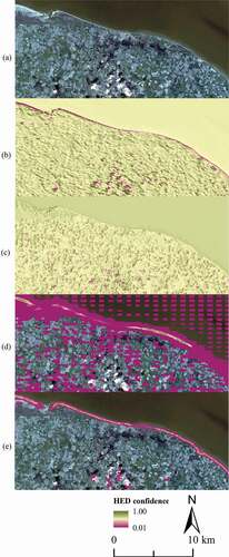
Figure 6. (a) Original 5 m RapidEye image of Varela, Guinea-Bissau (12°28ʹ61.0 N, −16°59ʹ45.7 E). Predicted coastal vegetation edge locations using the HED model trained with spectral band combination (b) RGB, (c) RG-NDVI, (d) RB-NIR, (e) RG-NIR.

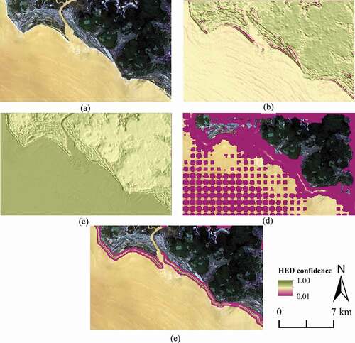
Figure 7. (a) Original 3 m PlanetScope image of the islands of Sylt, Amrum, and Föhr, Frisian Islands, Germany (54°68ʹ31.4 N, 8°55ʹ74.4 E). Predicted coastal vegetation edge locations using the HED model trained with spectral band combination (b) RGB, (c) RG-NDVI, (d) RB-NIR, (e) RG-NIR.

2.5. Shoreline change detection

The VEdge_Detector tool was used to predict the vegetation line from 11 images of Covehithe spanning the period 2010 to 2020. To minimize the influence of seasonal changes to vegetation line location, all selected images were captured in the period between May and August of each year. Confidence contours were generated at 0.1 intervals from 0.05 to 0.95, creating a total of 10 landward and seaward contours per image.

Vegetation line change was calculated using DSAS in ArcGIS 10.5.1 (USGS 2018). The position of the 10 confidence contours for every year was determined along transects running orthogonal to the dominant shoreline direction. Transects were separated by 10 m alongshore intervals. Change in the position of the landward and seaward 0.95, 0.55, and 0.05 confidence contours was calculated to determine rates of vegetation line change. Metrics calculated were Net Shoreline Change (NSC = distance between the oldest and most recent shoreline position) and End Point Rate (EPR = NSC divided by the time interval in years). To minimize geometric errors, ten tie-points were used to ensure consistent georegistration in the 11 images used in shoreline change analysis. The locations of stable anthropogenic structures, including road junctions and building corners, were used as the tie points and were distributed evenly over the images.

Aerial imagery of Covehithe, provided by the Environment Agency with 10 to 50 cm resolution, was manually digitized (Environment Agency, 2020). NSC values derived using DSAS were compared when using vegetation lines produced by the VEdge_Detector tool and manual digitization of aerial imagery. Due to aerial imagery availability, NSC values were compared across five baselines: 2010 to 2011, 2013 to 2014, 2015 to 2016, 2016 to 2017, and 2017 to 2018.

3. Results

3.1. Manual, ground-referenced, and VEdge_Detection measurements

Manually digitized vegetation lines were consistently located close to ground-referenced measurements (root mean square error (RMSE) was 1.72, 4.13, and 2.28 m for Covehithe, Walberswick (landward) and Dunwich, respectively). All sites exhibited a landward bias in manual digitization, with mean absolute error (MAE) of 0.82, 3.83, and 1.83 m, respectively. Across all sites, >93% of transects recorded an error ≤2 image pixels (6 m). At Walberswick, where ground-referenced measurements of two vegetation lines were collected, the manually digitized line was located closer to the landward continuous vegetation line than the seaward isolated vegetation patches (manual digitization to seaward measurements RMSE = 16.72 m and MAE = 13.83 m). VEdge_Detector performance was therefore subsequently compared to the landward ground-referenced measurements at Walberswick.

The VEdge_Detector tool extracted continuous vegetation edges at all three field sites (Figure 8). For every site the VEdge_Detector 0.95 confidence contours were <5 m from ground-referenced vegetation line measurements (see Table 2 for summary of all RMSE and MAE values).

Table 2. VEdge_Detector accuracy at the three field sites determined by pixel and distance-based metrics from ground-referenced measurements. Shaded pixels in the mean absolute error column represent a landward (green) or seaward (blue) bias respectively in VEdge_Detector predictions. Darker colours represent a greater landward or seaward bias. Red boxes indicate the confidence contours with lowest RMSE and MAE per site. VEdge_Detector outputs are shown in Figure 8

Figure 8. Comparison of VEdge_Detector tool predictions to field measurements of vegetation line at (a) Covehithe, (b) Walberswick, and (c) Dunwich. Locations of photograph (a)i, (b)i, and (c)i are show by arrows on corresponding images. The solid black lines show the ground-referenced vegetation lines at all sites. At Walberswick, the landward and seaward vegetation lines derived from field measurements are denoted by a solid and dashed line, respectively.

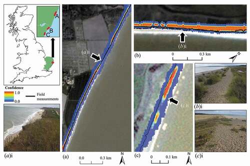
At Walberswick and Covehithe, all ground-referenced measurements were located between or seawards of the 0.95 confidence contours (Figure 8 (a) – (b)). The VEdge_Detector tool performed best at Covehithe with ground-referenced measurements located closest to the seaward 0.95 confidence contour (RMSE = 2.71 m, MAE = −0.02 m). A landward bias in the landward 0.95 contour (MAE = 7.98 m) and a seaward bias in the 0.95 seaward contour demonstrates that ground-referenced measurements at Covehithe were primarily located between the 0.95 confidence contours. Ground-referenced measurements were closest to the seaward 0.05 confidence contour at Walberswick (RMSE = 4.46 m, MAE = −1.11 m). Most ground-referenced measurements were situated between the seaward 0.95 (MAE = 4.31 m) and 0.05 confidence contours. The larger RMSE and MAE values for landward confidence contours compared to seaward contours shows a slight landward bias in VEdge_Detector outputs at Covehithe and Walberswick.

The relatively high P_A scores at these two sites (Covehithe = 0.87, Walberswick = 0.84) demonstrate that VEdge_Detector correctly detected a large proportion of vegetation line pixels derived from ground-referenced measurements. However, the lower U_A (Covehithe = 0.16 and Walberswick = 0.11) shows that a number of pixels inland of the field-derived vegetation line pixels are also being detected by the VEdge_Detector.

In contrast to the other two sites, VEdge_Detector predictions were primarily seawards of ground-referenced measurements at Dunwich (0.95 landwards confidence contour RMSE = 5.98 m, landward MAE = −5.21 m). The field line was located very close to the 0.05 confidence contour (RMSE = 2.37 m, MAE = 1.03 m). P_A values at Dunwich were consistent with the other two field sites, although a lower U_A was recorded (P_A = 0.85, U_A = 0.07).

The VEdge_Detector tool produced a continuous vegetation line at three of the four sites without field data (Figure 9). The tool failed to predict a continuous vegetation line along some cliffed sections at Perranuthnoe, but a continuous line was generated along the beach sections and the cliffed sections to the right of the image (Figure 9 (c)). The tool performed best at Winterton and Bribie Island with errors <4 m between 0.95 confidence contours and manually digitized lines (Winterton MAE = 3.83 m, Bribie Island MAE = 3.11 m, Figure 9 (a)–(b), Table 3). P_A values >0.9 were recorded at Winterton, Bribie Island, and Wilk-Ann-Zee, demonstrating a very high capability of the tool to detect the manually digitized vegetation line pixels. U_A was higher at Bribie (0.39) compared with Winterton (0.11), indicating that the tool produced a less precise line at Winterton.

Table 3. VEdge_Detector accuracy at the four validation sites without ground-referenced data determined by pixel and distance-based metrics. Shaded pixels in the mean absolute error column represents a landward (green) or seaward (blue) bias respectively in VEdge_Detector predictions. Darker colours represent a greater landward or seaward bias. Red boxes indicate the confidence contours with lowest RMSE and MAE per site. VEdge_Detector outputs are shown in Figure 9

Figure 9. VEdge_Detector outputs for (a) Winterton, Suffolk, UK (b) A stretch of Bribie Island, Australia, separate to the locations used for training outlined in the supplemental material, and (c) Perranuthnoe, Cornwall, UK. The red oval indicates the rocky cliff section where the VEdge_Detector failed to detect cliff top vegetation, (d) Wilk-Ann-zee, Netherlands. (a) and (b) display the predicted vegetation line in red with a confidence ≥0.95. (c) and (d) show examples of all VEdge_Detector outputs prior to applying any confidence thresholding. The white line in (c) and (d) shows the location of the manually digitized line.

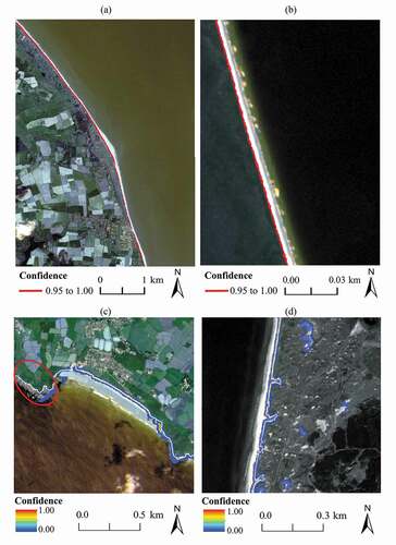
U_A and P_A were lower at Wilk-An-Zee and Perranuthnoe (Table 3), although more complex vegetation lines are found at these sites instead of straight sections. More inland pixels were predicted as the vegetation line at these sites (Figure 9 (c)–(d)). There was a greater seaward bias in tool predictions at Perranuthnoe (RMSE = 7.14 m, MAE = −6.63 m), whereas distance-based error at Wilk-Ann-Zee was comparable to Bribie and Winterton (RMSE = 4.61 m, MAE = 5.57 m).

3.2. Digital shoreline change analysis

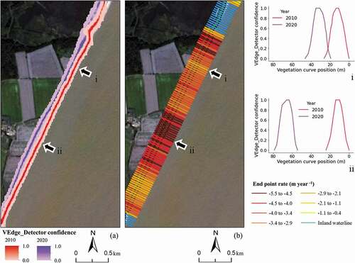
For Covehithe, the VEdge_Detector tool generated confidence curves of vegetation line position from separate images captured in 2010 and 2020 (Figure 10 (a)). A continuous shoreline was extracted from both images, including where the vegetation line is interrupted by the local shingle barriers that enclose Benacre Broad and Covehithe Broad. Total change in shoreline position between these two years was measured using the DSAS tool and the seaward 0.95 confidence contours (Figure 10 (b)). End point rates (EPR) along the Covehithe cliffs ranged between 2.47 and 5.48 m year⁻¹, with an average retreat rate of 3.27 m year⁻¹ (Figure 10(b)). The total amount of shoreline retreat during this period ranged between 24.27 and 54.38 m; the transect with the smallest and largest retreat are shown as location i and ii respectively in Figure 10 (a)–(b). Cross sections of the confidence curves at locations i and ii are shown in the two insets in Figure 10 (a). The stretches of shoreline with the greatest rates of retreat corresponded to areas with no overlap in confidence curves. In contrast, the confidence curves overlapped up to the 0.2 confidence contours at transects where retreat rates were lower.

Figure 10. (a) VEdge_Detector outputs for a 2010 (red) and 2020 (purple) image of the Covehithe cliffs, Suffolk. Darker colours represent pixels predicted as the vegetation line with a higher confidence. Inset graphs, comparison of vegetation curves at transects situated at location i (smallest recorded change in shoreline position) and ii (largest recorded retreat in shoreline). Note: The image shows VEdge_Detector outputs with confidence values from 0.01 to 1.00, whereas the graphs show values 0.05–1.00 because the line graphs substantially ‘fan’ between 0.01 and 0.05. (b) Rates of landward retreat (End Point Rate) at Covehithe between 2010 and 2020.

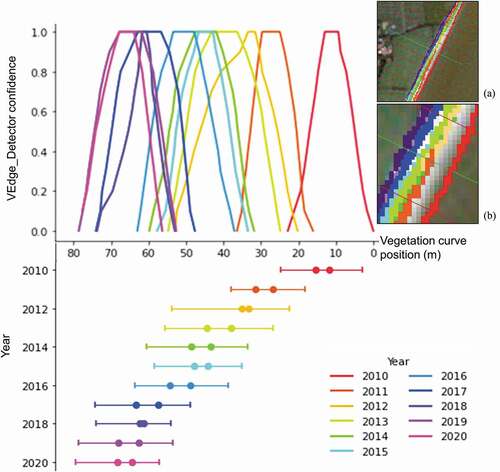
The VEdge_Detector tool was subsequently used to generate confidence curves of vegetation line position at Covehithe annually between 2010 and 2020. Continuous vegetation lines were generated in all years except 2011, 2012, and 2018 when some agricultural fields had been ploughed, leading to apparent breaks in the vegetation line. The relative position of the annual confidence curves from 2010 to 2020 at the location with the fastest rate of retreat is presented in Figure 11. The vegetation line retreated landwards at a faster rate during the first half of the decade (EPR 2010 to 2015 = 6.92 m year⁻¹, 2016 to 2020 = 4.31 m year⁻¹, Figure 11). Individual years with the greatest rates of landward retreat were 2010 to 2011 (16.1 m ± 3.67 m), 2016 to 2017 (8.80 ± 3.24 m), 2013 to 2014 (6.93 ± 4.20 m) and 2017 to 2018 (5.31 ± 3.38 m). The smallest retreat rates were recorded in 2014 to 2015 (1.66 ± 2.45 m) and 2018 to 2019 (1.32 ± 3.44 m). The greatest distance between 0.95 landward and seaward confidence contours was in 2013 (6.70 m) and the shortest distance was in 2018 (1.23 m).

Figure 11. Top: Vegetation confidence curve position during years 2010–2020 at one transect. Bottom: Representation of vegetation curves as a line. Dots represent locations of the 0.95 confidence contours, vertical lines represent locations of the 0.05 confidence contours. Insets i and ii: Transect location and all pixels predicted as the vegetation line with confidence >0.95 overlaid on the 2020 image. Pixel colour coding by year is consistent with line graphs. Some of the colours are occluded in the image due to overlap.

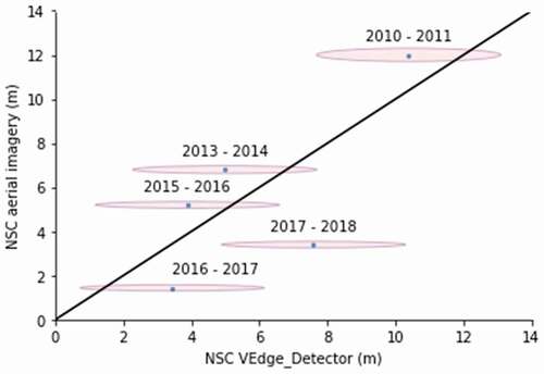
Net Shoreline Change (NSC) values derived using DSAS were averaged across the entire Covehithe coastline using both VEdge_Detector 0.95 confidence contours and manual digitization of aerial imagery. Differences in NSC values obtained using the two methods ranged between 1.31 and 4.19 m, with a mean absolute difference of 2.19 m (Figure 12). An error value of ± 2.71 m was used for VEdge_Detector outputs, the RMSE between VEdge_Detector 0.95 confidence contours and ground-referenced measurements at Covehithe. Errors from digitizing aerial imagery were set at 4.76% of each year’s NSC value, consistent with calculations of error determined using the same digitization method in Brooks and Spencer (2010).

Figure 12. Comparison of Net Shoreline Change (NSC) values generated the VEdge_Detector 0.95 confidence contours and manually digitized aerial imagery. The blue dots show annual NSC values for the whole of the Covehithe coastline averaged over all orthogonal transects. The ovals represent the error associated with the two methods. The black line shows the position of the blue dots if there was an exact match between NSC values generated using the two methods.

4. Discussion VEdge_Detector performance

VEdge_Detector is the first fully automated tool for the digitization of the coastal vegetation line from optical remote-sensing imagery, where a trained convolutional neural network (CNN) is used to detect the coastal vegetation line. The tool has been adapted from the holistically nested edge detection (HED) model (Xie and Tu 2015), a CNN trained to identify all objects in natural images. Here HED has been retrained to identify exclusively coastal vegetation edges, achieved by training the HED model on a comprehensive set of coastal remote-sensing images. At six of the seven validation sites, VEdge_Detector 0.95 confidence contours were <6 m from coastal vegetation edges derived from ground-referenced measurements or manual digitization of aerial imagery (Tables 2 and Tables 3). Previous studies have employed semi-automated methods to detect coastal vegetation, including thresholding and image classification (Zarillo, Kelley, and Larson 2008; Rahman et al., 2011). VEdge_Detector advances these studies by being able to identify the coastal vegetation line in isolation, without requiring further post-processing steps to remove inland vegetation land covers and edges.

VEdge_Detector differs from other shoreline change studies by exclusively using Planet imagery with 3 and 5 m spatial resolution. The combined high temporal and spatial resolution and coverage of Planet imagery provides a step-change in the ability to conduct shoreline change analysis. Previous studies have been primarily limited to digitizing shoreline position in Google Earth Engine’s Landsat or Copernicus imagery with 30 and 10 m resolution, respectively (Gorelick et al. 2017). Improvements in error values when using this imagery have been achieved using soft-classification, contouring and other methods with sub-pixel precision (Foody, Muslim, and Atkinson 2005; Li and Gong 2016; Pardo-Pascual et al. 2018). Extraction of the coastal vegetation line using imagery with 10–30 m resolution will remain problematic as one pixel can span the entire width of the coastal zone, incorporating numerous shoreline proxies. RMSE values derived in this study (2.37–7.97 m) are comparable or a substantial improvement to error values derived from sub-pixel precision methods applied to coarser resolution imagery.

The combination of the high (up to daily) temporal resolution of the Planet imagery with the VEdge_Detector tool gives new opportunities to analyse the horizontal change in shoreline position caused by an individual major storm event or a succession of storm events (Roy 2017). Previously this has only been possible through field or aerial-based studies (e.g. Spencer et al. 2015). Studies of this nature are rare because data collection methods are time consuming, costly and information on shoreline position and profile prior to the storm event is only available in isolated, data-rich areas. The passive nature of image data collection used in VEdge_Detector, combined with its high spatio-temporal resolution opens new possibilities to assess storm damage, or other discrete erosion or accretion events in relatively understudied or inaccessible areas.

VEdge_Detector performed best on relatively simple, straight stretches of shoreline (e.g. Covehithe, Winterton and Bribie Island; Figure 8 (a)–(b)). Perranuthnoe, Cornwall, UK, was the only location where VEdge_Detector did not generate a continuous vegetation line. This can be primarily attributed to the additional presence of rocky cliffs, because the majority of training data images contained only beaches. While additional HED training using more images containing rocky cliffed shorelines may improve model performance, this may be at the expense of performance along sandy beached sections. Figure 9 (c) shows that the tool can detect a vegetation line at the base of some of the cliffs at Perranuthnoe, possibly due to the presence of macroalgae on the shore platform. It is beyond the scope of VEdge_Detector to include these sections, because change in macroalgal cover is highly unlikely to reflect an actual landward or seaward migration in shoreline position. Similarly, fixed coastal defences will not contain a mobile vegetation edge. Hence it is important to note that VEdge_Detector is primarily a tool for efficient and rapid extraction of the vegetation line from beach and dune systems over wide spatial coverage, from which shoreline change analysis can be performed.

The small discrepancies presented here between manually digitized shorelines and ground-referenced measurements from the first three cases studies provided confidence in using manually digitized shorelines to assess VEdge_Detector performance at several alternative sites where ground-referenced measurement was not possible (RMSE = 1.72, 4.13, and 2.28 m for Covehithe, Walberswick (landwards) and Dunwich, respectively). At Walberswick, the manually digitized line was closer to the landward field vegetation line measurements, indicating that manual digitization primarily detects the more continuous vegetation line boundary landwards of the habitat of pioneer species. It appears that the diffuse nature of the vegetation edge in some locations, with isolated, dis-continuous vegetation clumps, can lead to discrepancies between manual digitization, ground-referenced measurements, and VEdge_Detector results because the best available imagery is of 3–5 m resolution.

This study further showed that the method was robust at detecting the vegetation line on both tropical and temperate coasts. To date, the only previous use of CNNs to extract shoreline position has been limited to a single location (X.Y. Liu et al. 2019). Results presented here for seven different validation sites have shown that at six sites, P_A was above 0.85, but U_A was lower than P_A at every site (Tables 2 and Tables 3). This demonstrates how the tool is competent at correctly predicting the vegetation line pixel derived from ground referenced measurements but also generates a vegetation boundary region instead of a distinct line. These performance metrics are lower than those recorded by X.Y. Liu et al. (2019) (U_A = 0.94, P_A = 0.95). However, X.Y. Liu et al. (2019) used far coarser spatial resolution imagery (16 m to 50 m) and thus poorer U_A and P_A results presented here could still result in lower RMSE values. Confidence contours were used throughout this study to determine where ground referenced measurements were located across predicted vegetation line confidence curves. At six of the seven sites, ground referenced measurements were closest to one of the 0.95 confidence contours, with RMSE <6 m (Figures 8 and 9). This highlights that even though a distinct vegetation line is not predicted, VEdge_Detector commonly predicts the ground referenced vegetation line with higher confidence than the surrounding pixels.

Vegetation lines were predicted with higher U_A along shorelines with abrupt vegetation edges. The fieldwork and additional validation sites with the highest U_A results were Covehithe (U_A = 0.16) and Bribie Island (U_A = 0.38) respectively. Bribie Island has an abrupt vegetation line as bare sand is found immediately adjacent to eucalyptus forest and Covehithe has an abrupt cliff-top vegetation boundary because cliff line retreat is too rapid for cliff toe vegetation establishment. In comparison, VEdge_Detector U_A results were lower at Dunwich (U_A = 0.07), Walberswick (U_A = 0.11), and Wilk-Ann-Zee (U_A = 0.07), which all contain graded psammosere community vegetation on beach dune systems. The low U_A and higher P_A results highlight how the vegetation edge is not a true line, but a boundary region graded from no vegetation to increasingly dense vegetation when traversing inland. Discrepancies in the interpretation of vegetation line position occur even when collating ground-referenced measurements. This was demonstrated at Walberswick, where P_A increased from 0.59, when using the most seaward pioneer vegetation, to 0.84 when using the landward continuous vegetation edge (Figure 8 (b), Table 2). Further investigation, supported with ground-referenced measurements, is required to determine whether this tool not only identifies vegetation edge location but also whether U_A results can indicate the degree of abrupt change in a vegetation boundary. An increase in vegetation line ‘abruptness’ can imply a loss of pioneer species seaward of dune systems, perhaps as a result of erosion under storm impacts or wave action associated with particularly high tides. Conversely, increasing widths in vegetation edge can represent relatively stable, or prograding, shoreline locations where vegetation has had the opportunity to establish and migrate seawards.

This paper also provides the first-ever comparison of the performance of a HED model using different spectral band combinations. RG-NIR visually outperformed other spectral band combinations, demonstrating the importance of spectral band selection in HED training. This finding is complementary to the universally applied vegetation detection algorithm, NDVI, which utilizes the near-infrared and red wavebands (Genovese et al. 2001). HED and many other CNN architectures only allow the input of images with three spectral bands (Simonyan and Zisserman 2014). Improved performance may be achieved by concatenating the outputs of multiple CNNs trained on three band images. Marmanis et al. (2018) fused the outputs of two CNNs run in parallel, one CNN trained using spectral band information and the other trained using digital terrain models. Parallel CNNs were reported to automatically classify land covers with 84.8% pixel accuracy, but no comparison to single CNN performance was provided. Further investigations should compare the performance of single and multiple parallel CNNs trained exclusively on images with different spectral band combinations.

4.1. Shoreline change analysis using VEdge_Detector

The VEdge_Detector tool showed predicted a consistent landward shift in vegetation position between 2010 and 2020 at Covehithe, Suffolk (Figure 10). Years when the VEdge_Detector recorded the greatest rates of landward retreat coincide with North Sea storm surge events in December 2013 (Spencer et al. 2015; Wadey et al. 2015) and January 2017 (Floodlist 2017) and the February to March 2018 ‘Beast from the East’ and ‘mini-Beast’ (Brooks and Spencer 2019). Average rates of landward retreat at Covehithe derived from VEdge_Detector were consistent with results obtained in this study from manually digitizing aerial imagery. The mean difference in NSC values when using VEdge_Detector and digitizing aerial imagery was less than one pixel. These NSC values are also complementary to values derived along this stretch of shoreline using other proxy and datum-based methods (Brooks and Spencer, 2012; Burningham and French 2017). This study has demonstrated the aptitude for the VEdge_Detector tool to accurately and efficiently detect the vegetation line from a relatively data-rich shoreline where it has been possible to use other measurements, including aerial imagery, lidar data and Ordinance Survey data, to validate precision. Further applications of this tool should investigate its use in relatively data poor regions of the world or in regions where there is a necessity to determine the impact of coastal protection schemes or other anthropogenic interventions in the coastal zone.

A continuous vegetation line was generated at Covehithe for 8 out of 11 years. During 3 years, the vegetation line was fragmented due to the presence of ploughed agricultural land which interrupted the vegetation line. VEdge_Detector has been shown to be able to overcome issues of vegetation line fragmentation in other images, for example detecting the landward extent of Benacre Broad and Covehithe Broad on the Suffolk coast (Figure 10 (a)). Further studies should increase the ability for the tool to generalize, and use urban and water pixels when the vegetation line is fragmented. Alongside the sometimes fragmented nature of the vegetation line, it may remain an unsuitable proxy to use in shoreline change analysis in circumstances where there have been changes in vegetation communities as a result of both natural and anthropogenic processes unrelated to shoreline position. Therefore, this paper suggests future research should combine multiple shoreline proxies simultaneously to provide a better indication of shoreline change.

5. Conclusion

This study has trained a holistically nested edge detection (HED) model to produce VEdge_Detector, a fully automated tool for the extraction of coastal vegetation lines along sandy shorelines from optical remote-sensing imagery. The semantic knowledge gained during HED training enables VEdge_Detector to discriminate between coastal vegetation edges and other inland vegetation boundaries, thus only extracting the coastal vegetation line and removing the need for subsequent post-processing. VEdge_Detector produces a vegetation confidence curve instead of a discrete line, which better represents how, in reality, the coastal vegetation line is not a distinct boundary but a broad zone where vegetation becomes a more continuous cover when traversing inland. The low error values (RMSE <6 m at all sites) between VEdge_Detector predictions and ground-referenced measurements demonstrate the aptitude for this tool to accurately detect the coastal vegetation edge location. VEdge_Detector performance varied depending on spectral band selection, with red, green and near-infrared shown to be the most pertinent image bands to use for coastal vegetation edge detection. This highlights the importance of image spectral band selection during CNN training in any context.

VEdge_Detector has been used to detect a decadal-scale, consistent landward shift in shoreline position at Covehithe, Suffolk, UK. This trend in vegetation line position is consistent with measurements obtained through manually digitizing aerial imagery. This exemplifies how using this tool at different locations, which exhibit a larger horizontal tidal range, may produce a more robust proxy of shoreline position than using the waterline to determine net shoreline change. The Planet imagery used to train the VEdge_Detector tool has sufficient spatio-temporal resolution to investigate the impacts of individual storm events along highly erodible shorelines or human management interventions on shoreline position. The high global coverage of this imagery opens new opportunities for shoreline change analysis in otherwise data-poor regions of the world.

Acknowledgements

The aerial imagery provided is courtesy of the UK Environment Agency. This work was funded through the UKRI NERC/ESRC Data, Risk and Environmental Analytical Methods (DREAM) Centre for Doctoral Training, Grant/Award Numbers: NE/M009009/1, NE/R011265/1 and is a contribution to UKRI NERC BLUECoast (NE/N015924/1; NE/N015878/1). The authors would like to thank Prof. Iris Möller (Trinity College Dublin) for her contributions towards developing the research objective.

Disclosure statement

No potential conflict of interest was reported by the authors.

Additional information

Funding

This work was supported by the the UKRI NERC/ESRC Data, Risk and Environmental Analytical Methods (DREAM) Centre for Doctorial Training [NE/M009009/1, NE/R011265/1]; BLUECoast [NE/N015878/1,NE/N015924/1].

References

- Almonacid-Caballer, J., E. Sánchez-García, J. E. Pardo-Pascual, A. A. Balaguer-Beser, and J. Palomar-Vázquez. 2016. “Evaluation of Annual Mean Shoreline Position Deduced from Landsat Imagery as a Mid-term Coastal Evolution Indicator.” Marine Geology 372: 79–88. doi:https://doi.org/10.1016/j.margeo.2015.12.015.
- Arbelaez, P., C. Fowlkes, and M. Martin 2007. “The Berkeley Segmentation Dataset and Benchmark.” Available at: https://www2.eecs.berkeley.edu/ Accessed 13 January 2020
- Bayram, B., F. Erdem, B. Akpinar, A. K. Ince, S. Bozkurt, H. C. Reis, and D. Z. Seker. 2017. “The efficiency of random forest method for shoreline extraction from LANDSAT-8 and GOKTURK-2 imageries.” ISPRS Annals of the Photogrammetry, Remote Sensing and Spatial Information Sciences 4: 141–145. doi:https://doi.org/10.5194/isprs-annals-IV-4-W4-141-2017.
- Boak, E. H., and I. L. Turner. 2005. “Shoreline definition and detection: a review.” Journal of Coastal Research 214: 688–703. doi:https://doi.org/10.2112/03-0071.1.
- Breiman, L. 2001. “Random forests.” Machine Learning 45 (1): 5–32. doi:https://doi.org/10.1023/A:1010933404324.
- Brock, J. C., and S. J. Purkis. 2009. “The emerging role of LiDAR remote sensing in coastal research and resource management.” Journal of Coastal Research 53: 1–5. doi:https://doi.org/10.2112/SI53-001.1.
- Brooks, S., and T. Spencer, 2019. “Long-term Trends, Short-term Shocks and Cliff Responses for Areas of Critical Coastal Infrastructure.” In Coastal Sediments 2019: Proceedings of the 9th International Conference, (pp. 1179–1187). Tampa, Florida, USA.
- Brooks, S. M., and T. Spencer. 2010. “Temporal and Spatial Variations in Recession Rates and Sediment Release from Soft Rock Cliffs, Suffolk Coast, UK.” Geomorphology 124 (1–2): 26–41. doi:https://doi.org/10.1016/j.geomorph.2010.08.005.
- Burningham, H., and J. French. 2017. “Understanding Coastal Change Using Shoreline Trend Analysis Supported by Cluster-based Segmentation.” Geomorphology 282: 131–149. doi:https://doi.org/10.1016/j.geomorph.2016.12.029.
- Cefas, 2020. “WaveNet Interactive Map.” [online] Available at: http://wavenet.cefas.co.uk/Map [ Accessed 21 May 2020].
- Choung, Y. J., and M. H. Jo. 2017. “Comparison between a Machine-learning-based Method and a Water-index-based Method for Shoreline Mapping Using a High-resolution Satellite Image Acquired in Hwado Island, South Korea.” Journal of Sensors 2017: 1–13. doi:https://doi.org/10.1155/2017/8245204.
- Committee on Climate Change, 2018. “Managing the Coast in a Changing Climate.” Available online: https://www.theccc.org.uk/publication/managing-the-coast-in-a-changing-climate/(accessed 14 March 2020
- De Andrés, M., J. M. Barragán, and M. Scherer. 2018. “Urban Centres and Coastal Zone Definition: Which Area Should We Manage?” Land Use Policy 71: 121–128. doi:https://doi.org/10.1016/j.landusepol.2017.11.038.
- Demir, N., S. Oy, F. Erdem, D. Z. Şeker, and B. Bayram. 2017. “Integrated Shoreline Extraction Approach with Use of Rasat MS and SENTINEL-1A SAR Images.” ISPRS Annals of the Photogrammetry, Remote Sensing and Spatial Information Sciences 4: 445–449. doi:https://doi.org/10.5194/isprs-annals-IV-2-W4-445-2017.
- Elnabwy, M. T., E. Elbeltagi, M. M. El Banna, M. M. Elshikh, I. Motawa, and M. R. Kaloop. 2020. “An Approach Based on Landsat Images for Shoreline Monitoring to Support Integrated Coastal Management—A Case Study, Ezbet Elborg, Nile Delta, Egypt.” ISPRS International Journal of Geo-Information 9 (4): 199–218. doi:https://doi.org/10.3390/ijgi9040199.
- Environment Agency, 2020. “Vertical Aerial Photography.” Available online: https://data.gov.uk/dataset, (accessed 19 June 2020
- Ferreira, O., T. Garcia, A. Matias, R. Taborda, and J. A. Dias. 2006. “An Integrated Method for the Determination of Set-back Lines for Coastal Erosion Hazards on Sandy Shores.” Continental Shelf Research 26 (9): 1030–1044. doi:https://doi.org/10.1016/j.csr.2005.12.016.
- Floodlist., 2017. “UK – Storm Surge Causes Flooding Along England’s East Coast.” Available online: www.http://floodlist.com/europe/united-kingdom (accessed 17 June 2020
- Foody, G. M., A. M. Muslim, and P. M. Atkinson. 2005. “Super‐resolution Mapping of the Waterline from Remotely Sensed Data.” International Journal of Remote Sensing 26 (24): 5381–5392. doi:https://doi.org/10.1080/01431160500213292.
- Genovese, G., C. Vignolles, T. Nègre, and G. Passera. 2001. “A Methodology for A Combined Use of Normalised Difference Vegetation Index and CORINE Land Cover Data for Crop Yield Monitoring and Forecasting. A Case Study on Spain.” Agronomie 21 (1): 91–111. doi:https://doi.org/10.1051/agro:2001111.
- Gorelick, N., M. Hancher, M. Dixon, S. Ilyushchenko, D. Thau, and R. Moore. 2017. “Google Earth Engine: Planetary-scale Geospatial Analysis for Everyone.” Remote Sensing of Environment 202: 18–27. doi:https://doi.org/10.1016/j.rse.2017.06.031.
- Hagenaars, G., S. De Vries, A. P. Luijendijk, W. P. De Boer, and A. J. Reniers. 2018. “On the Accuracy of Automated Shoreline Detection Derived from Satellite Imagery: A Case Study of the Sand Motor Mega-scale Nourishment.” Coastal Engineering 133: 113–125. doi:https://doi.org/10.1016/j.coastaleng.2017.12.011.
- Kokkinos, I., 2015. “Pushing the Boundaries of Boundary Detection Using Deep Learning. arXiv Preprint.” arXiv:1511.07386.
- Lab, S. V., 2016. “ImageNet. [Online].” Available at http://www.image-net.org/ [Accessed 18 November 2019
- Li, W., and P. Gong. 2016. “Continuous Monitoring of Coastline Dynamics in Western Florida with a 30-year Time Series of Landsat Imagery.” Remote Sensing of Environment 179: 196–209. doi:https://doi.org/10.1016/j.rse.2016.03.031.
- Liu, C. (2018). “HED: Keras Implementation.” Github repository https://github.com/lc82111
- Liu, H., J. Luo, Y. Sun, L. Xia, W. Wu, H. Yang, X. Hu, and L. Gao, 2019. “Contour-oriented Cropland Extraction from High Resolution Remote Sensing Imagery Using Richer Convolution Features Network.” In 2019 8th International Conference on Agro-Geoinformatics (Agro-Geoinformatics). IEEE : 1–6. Istanbul, Turkey.
- Liu, X. Y., R. S. Jia, Q. M. Liu, C. Y. Zhao, and H. M. Sun. 2019. “Coastline Extraction Method Based on Convolutional Neural Networks—A Case Study of Jiaozhou Bay in Qingdao, China.” IEEE Access 7: 180281–180291. doi:https://doi.org/10.1109/ACCESS.2019.2959662.
- Lu, T., D. Ming, X. Lin, Z. Hong, X. Bai, and J. Fang. 2018. “Detecting Building Edges from High Spatial Resolution Remote Sensing Imagery Using Richer Convolution Features Network.” Remote Sensing 10 (9): 1496–1515.
- Luijendijk, A., G. Hagenaars, R. Ranasinghe, F. Baart, G. Donchyts, and S. Aarninkhof. 2018. “The State of the World’s Beaches.” Scientific Reports 8: 6641.
- Marmanis, D., K. Schindler, J. D. Wegner, S. Galliani, M. Datcu, and U. Stilla. 2018. “Classification with an Edge: Improving Semantic Image Segmentation with Boundary Detection.” ISPRS Journal of Photogrammetry and Remote Sensing 135: 158–172. doi:https://doi.org/10.1016/j.isprsjprs.2017.11.009.
- McFeeters, S. K. 1996. “The Use of the Normalized Difference Water Index (NDWI) in the Delineation of Open Water Features.” International Journal of Remote Sensing 17 (7): 1425–1432. doi:https://doi.org/10.1080/01431169608948714.
- Mentaschi, L., M. I. Vousdoukas, J.-F. Pekel, E. Voukouvalas, and L. Feyen. 2018. “Global Long-term Observations of Coastal Erosion and Accretion.” Scientific Reports 8 (1): 12876. doi:https://doi.org/10.1038/s41598-018-30904-w.
- Mohajerani, Y., M. Wood, I. Velicogna, and E. Rignot. 2019. “Detection of Glacier Calving Margins with Convolutional Neural Networks: A Case Study.” Remote Sensing 11 (1): 74–87. doi:https://doi.org/10.3390/rs11010074.
- Moore, L. J., P. Ruggiero, and J. H. List. 2006. “Comparing Mean High Water and High Water Line Shorelines: Should Proxy-datum Offsets Be Incorporated into Shoreline Change Analysis?” Journal of Coastal Research 224: 894–905. doi:https://doi.org/10.2112/04-0401.1.
- Pardo-Pascual, J. E., E. Sánchez-García, J. Almonacid-Caballer, J. M. Palomar-Vázquez, E. Priego De Los Santos, A. Fernández-Sarría, and Á. Balaguer-Beser. 2018. “Assessing the Accuracy of Automatically Extracted Shorelines on Microtidal Beaches from Landsat 7, Landsat 8 and Sentinel-2 Imagery.” Remote Sensing 10 (2): 326–346. doi:https://doi.org/10.3390/rs10020326.
- Pardo-Pascual, J. E., J. Almonacid-Caballer, L. A. Ruiz, and J. Palomar-Vázquez. 2012. “Automatic Extraction of Shorelines from Landsat TM and ETM+ Multi-temporal Images with Subpixel Precision.” Remote Sensing of Environment 123: 1–11. doi:https://doi.org/10.1016/j.rse.2012.02.024.
- Pekel, J. F., A. Cottam, N. Gorelick, and A. S. Belward. 2016. “High-resolution Mapping of Global Surface Water and Its Long-term Changes.” Nature 540 (7633): 418–422. doi:https://doi.org/10.1038/nature20584.
- Planet Team, P. 2017. Planet Application Program Interface: In Space for Life on Earth. San Francisco: CA. https://api.planet.com
- Pollard, J. A., S. M. Brooks, and T. Spencer. 2019a. “Harmonising Topographic & Remotely Sensed Datasets, a Reference Dataset for Shoreline and Beach Change Analysis.” Nature Scientific Data 6 (1): 1–42.
- Pollard, J. A., T. Spencer, and S. M. Brooks. 2019b. “The Interactive Relationship between Coastal Erosion and Flood Risk.” Progress in Physical Geography: Earth and Environment 43 (4): 574–585. doi:https://doi.org/10.1177/0309133318794498.
- Pugh, D., and P. Woodworth. 2014. Sea-level Science: Understanding Tides, Surges, Tsunamis and Mean Sea-level Changes. Cambridge, UK: Cambridge University Press.
- Pye, K., and S. J. Blott. 2006. “Coastal Processes and Morphological Change in the Dunwich-Sizewell Area, Suffolk, UK.” Journal of Coastal Research 22 (3): 453–473. doi:https://doi.org/10.2112/05-0603.1.
- Rahman, A. F., D. Dragoni, and B. El-Masri. 2011. “Response of the Sundarbans Coastline to Sea Level Rise and Decreased Sediment Flow: A Remote Sensing Assessment.” Remote Sensing of Environment 115 (12): 3121–3128. doi:https://doi.org/10.1016/j.rse.2011.06.019.
- Ren, X. 2008. “Multi-scale Improves Boundary Detection in Natural Images”, In Forsyth, D., P. Torr, and Zisserman, A. (Eds.), European Conference on Computer Vision, 533–545. Springer: Heidelberg.
- Roy, S., 2017. “Planet to Google Earth Engine Pipeline (Command Line Interface).”
- Simonyan, K., and A. Zisserman, 2014. “Very Deep Convolutional Networks for Large-scale Image Recognition.” arXiv preprint arXiv:1409.1556.
- Spencer, T., S. M. Brooks, B. R. Evans, J. A. Tempest, and I. Möller. 2015. “Southern North Sea Storm Surge Event of 5 December 2013: Water Levels, Waves and Coastal Impacts.” Earth-Science Reviews 146: 120–145. doi:https://doi.org/10.1016/j.earscirev.2015.04.002.
- Thieler, E. R., E. A. Himmelstoss, J. L. Zichichi, and A. Ergul, 2009. “Digital Shoreline Analysis System (DSAS) Version 4.0 – An ArcGIS Extension for Calculating Shoreline Change.” US Geological Survey Open-file Report, 2008–1278. US Geological Survey, Reston, VA.
- Toure, S., O. Diop, K. Kpalma, and A. S. Maiga. 2019. “Shoreline Detection Using Optical Remote Sensing: A Review.” ISPRS International Journal of Geo-Information 8 (2): 75. doi:https://doi.org/10.3390/ijgi8020075.
- USGS, 2018. “Digital Shoreline Analysis System (DSAS).Version 5.0 User Guide.” Available online: https://www.usgs.gov/centers/whcmsc/science/digital-shoreline-analysis-system-dsas?qt-science_center_objects=0#qt-science_center_objects (accessed 15 April 2020
- Vos, K., M. D. Harley, K. D. Splinter, J. A. Simmons, and I. L. Turner. 2019. “Sub-annual to Multi-decadal Shoreline Variability from Publicly Available Satellite Imagery.” Coastal Engineering 150: 160–174. doi:https://doi.org/10.1016/j.coastaleng.2019.04.004.
- Wadey, M. P., I. D. Haigh, R. J. Nicholls, J. M. Brown, K. Horsburgh, B. Carroll, S. L. Gallop, T. Mason, and E. Bradshaw. 2015. “A Comparison of the 31 January – 1 February 1953 and 5 – 6 December 2013 Coastal Flood Events around the UK.” Frontiers in Marine Science 2: 84–111. doi:https://doi.org/10.3389/fmars.2015.00084.
- Xie, S., and Z. Tu, 2015. “Holistically-nested Edge Detection.” Proceedings of the IEEE International Conference on Computer Vision. 1395–1403. Santiago, Chile.
- Zarillo, G. A., J. Kelley, and V. Larson, 2008. “A GIS Based Tool for Extracting Shoreline Positions from Aerial Imagery (Beachtools) Revised (No. ERDC/CHL-CHETN-IV-73).” Engineer research and development center Vicksburg MS coastal and hydraulics lab.
- Zhang, H., Q. Jiang, and J. Xu. 2013. “Coastline Extraction Using Support Vector Machine from Remote Sensing Image.” Journal of Multimedia 8 (2): 175–182.
- Zhang, L., L. Zhang, and B. Du, 2016. “Deep Learning for Remote Sensing Data: A Technical Tutorial on the State of the Art.” IEEE Geoscience and Remote Sensing Magazine 4, 22–40.