The feasibility of using a low-cost near-infrared, sensitive, consumer-grade digital camera mounted on a commercial UAV to assess Bambara groundnut yield

ABSTRACT

Accurate, timely, and non-destructive early crop yield prediction at the field scale is essential in addressing changing crop production challenges and mitigating impacts of climate variability. Unmanned aerial vehicles (UAVs) are increasingly popular in recent years for agricultural remote sensing applications such as crop yield forecasting and precision agriculture (PA). The objective of this study was to evaluate the performance of a low-cost UAV-based remote sensing technology for Bambara groundnut yield prediction. A multirotor UAV equipped with a near-infrared sensitive consumer-grade digital camera was used to collect image data during the 2018 growing season (April to August). Flight missions were carried out six times during critical phenological stages of the life-cycle of the monitored crop. Yield was recorded at harvest. Four vegetation indices (VIs) namely normalized difference vegetation index (NDVI), enhanced vegetation index 2 (EVI2), green normalized difference vegetation index (GNDVI), and simple ratio (SR) generated from the Red-Green-Near Infrared bands were calculated using the georeferenced orthomosaic UAV images. Pearson’s product-moment correlation coefficient (r) and Bland–Altman testing showed a significant agreement between remotely and proximally sensed VIs. Significant and positive correlations were found between the four VIs and yield, with the strongest relationship observed between SR and yield at podfilling stage (r = 0.81, P < 0.01). Multi-temporal accumulative VIs improved yield prediction significantly with the best index being ∑SR and the best interval being from podfilling to maturity (r = 0.88, P < 0.01). The accumulated ∑SR from podfilling to maturity resulted in higher prediction accuracy with a coefficient of determination (R²) of 0.71, root mean square error (RMSE) of 0.20 and mean absolute percentage error (MAPE) of 14.2% than SR spectral index at a single stage (R² = 0.68, RMSE = 0.24, MAPE = 15.1%). Finally, a yield map was generated using the model developed, to better understand the within-field spatial variations of yield for future site-specific or variable-rate application operations.

1. Introduction

Food production must be substantially increased to meet global food demand in response to the exponentially growing world population and climate change (Fróna, Szenderák, and Harangi-Rákos 2019). A key strategy to adapt to ever-changing climatic conditions is the development and promotion of underutilized crop species which has great potential to improve food and nutrition security, diversify agriculture and reduce environmental impacts (Massawe et al. 2015). Bambara groundnut (Vigna subterannea) is one such indigenous African legume with enhanced ability to adapt to environmental stress and high yield stability under different environmental conditions, and thus can contribute to nutritional and food security (Massawe et al. 2005). Bambara groundnut yield forecasting prior to harvest allow governments to develop and implement national food policies, and is important for national food security and personal living standards. Other benefits include planning resource needs, optimization of harvest logistics, transport, and storage capacity (Zhou et al. 2017). Traditional methods of crop yield prediction usually rely on multiple field surveys, which are costly, time-consuming, and error-prone (Reynolds et al. 2000). Therefore, development of a low-cost, fast, and accurate method for Bambara groundnut yield prediction at a local scale is the main goal for crop production (Zhou et al. 2017).

Remote sensing is a key high-performance technology that allows; for precision agriculture (PA), non-destructive data collection, high throughput phenotyping, and is fast and reliable (Araus and Cairns 2014). The first use of satellites for remote sensing of vegetation goes back to the first National Aeronautics and Space Administration (NASA) Landsat series in the 1970s (Tucker 1979). Since then, the application of remote sensing for vegetation mapping has been constantly developing and several different indices calculated from specific wavelengths have been used to estimate plant growth parameters and crop yield (White et al. 2012). More recently, remote sensing technology has been extended to successfully predict vegetation biophysical attributes like leaf area index (LAI) (Potgieter et al. 2017), biomass (Wang et al. 2016), chlorophyll content (Haboudane et al. 2002), and has also been used for yield prediction of several crops such as soybean (Glycine max L.) (Yu et al. 2016), rice (Oryza sativa L.) (Zhou et al. 2017), and wheat (Triticum aestivum L.) (Du et al. 2017). Vegetation mapping was achieved through the use of numerous vegetation indices (VIs) such as normalized difference vegetation index (NDVI), enhanced vegetation index (EVI), optimized soil adjusted vegetation index (OSAVI), transformed chlorophyll absorption reflectance index (TCARI), green normalized difference vegetation index (GNDVI), amongst others, derived from visible and near infrared reflectance spectra at varying spatial, and temporal resolutions across large scales (Huete et al. 2002). Generally, the visible red (665–700), green (555–580), and near-infrared NIR (840–900) nm wavelengths provide important information regarding vegetation (Clevers 1989).

Traditional remote sensing platforms such as satellite and aircraft are continuously improving their spatial and temporal resolution, thus enhancing their suitability for PA. Each of these remote sensing technologies has advantages and disadvantages in terms of their technological, operational, and economic factors. For instance, satellite can map large areas at the same time, however, suffer from coarse resolution for PA purposes (Matese et al. 2015). Moreover, satellite surveys may be impeded by atmospheric effects such as cloud cover and aerosols and have long revisit period which might not coincide with specific phenological growth stages of the monitored vegetation (Zhang et al. 2019). There is more flexibility in planning aircraft surveys, however, it can be very difficult as it requires highly technical personnel to operate and involves costly campaign organization efforts. Unmanned aerial vehicles (UAVs) have limited payload and short flight endurance that makes them unsuitable for large area PA. However, UAVs are ideal to acquire high-resolution data from asmall field-scale area suitable for PA as well as research applications (Matese et al. 2015). UAVs are increasingly ubiquitous due to their numerous advantages which include high spatial/temporal flexibility, optimal cloud cover independence, useful for quick land surveying, low costs, ease of operation, minimal image processing, high spatial resolution, timely, and non-destructive data acquisition (Deng et al. 2018). Moreover, UAVs can be fitted with a variety of sensors such as digital, multispectral, hyperspectral, thermal, light detection and ranging (LIDAR), and synthetic aperture radar (SAR) for PA applications.

In the past decade, there is growing interest to integrate lightweight inexpensive consumer grade digital camera on UAVs for PA. Commercial consumer grade digital cameras have high spatial resolution, small ground sampling distance, and digital images captured can be used to generate high-quality dense point clouds for digital surface model and generation of orthomosaics (Toth and Grzegorz 2016). VIs derived from red green blue (RGB) digital orthophotos collected by consumer-grade digital camera have been used in soil mapping and sampling (Huuskonen and Oksanen 2018), fruit recognition and detection (Nyarko et al. 2018), early detection of water stress (Zhuang et al. 2017), monitoring plant condition, and phenology (Nijland et al. 2014). However, vegetation is highly sensitive to red (R) and near-infrared (NIR) bands and VIs based on red and near infrared bands have high performance in crop monitoring (Mutanga and Skidmore 2004). VIs derived from the red and near infrared bands are more widely used because of the characteristic difference between chlorophyll pigment absorptions in the red versus the high reflectance in the near infrared (Plummer 1988; Gitelson and Merzlyak 1997). A digital RGB camera can capture NIR band when the NIR filter is removed (Nijland et al. 2014). The result is a modified three-band digital consumer-grade camera capable of detecting two visible bands and one NIR band. Therefore, some research used modified digital camera to obtain information in the visible and NIR bands required to compute important VIs.

Berra, Gaulton, and Barr (2017) monitored the multi-temporal change in vegetation reflectance and NDVI using a low-cost modified commercial digital camera. Comparison of low-cost modified digital camera data with Landsat 8 satellite data showed relationships of 0.73 ≤ R² ≥ 0.84 for broadband surface reflectance and 0.86 ≤ R² ≥ 0.89 for NDVI, thus proving the suitability of modified digital camera for obtaining accurate vegetation reflectance and NDVI data. Sankaran et al. (2018) used a small octocopter equipped with a modified multispectral camera (NIR-Green-Blue) for high throughput phenotyping of a bean (Phaseolus vulgaris L.) field. They found out that GNDVI at mid-podfilling stage was significantly correlated with seed yield, while GNDVI at flowering and mid-podfilling was significantly correlated with biomass. Daughtry, Gallo, and Bauer (1983) proposed that correlation between grain yield and VIs obtained on a single date must be used with caution and that the cumulative additive of the VIs during the crop cycle may better account for crop yield. Du et al. (2017) used cumulative colour indices derived from images captured from a UAV to map within field spatial variations of wheat yield and also to monitor the wheat growth status on a winter wheat farmland in Hokkaido, Japan. Zhou et al. (2017) also reported that multi-temporal cumulative VIs performed better for rice yield prediction than single-stage VIs did in Jiangsu province, China. Jaafar and Ahmad (2015) predicted cotton (Gossypium sp.) yield of Hama province in Syria from cumulative EVI (R² = 0.77). Many other researchers have used cumulative VIs acquired throughout several phenological stages to predict yield in wheat (Wang et al. 2014), grape (Sun et al. 2017), maize (Mkhabela, Mkhabela, and Mashinini 2005) and rice (Huang et al. 2013). However, the concept of using cumulative VIs to predict yield of crops with underground pods has not yet been evaluated before thus warranting our study.

Although spectral reflectance indices have been thoroughly used to assess yield on different cereal crops as mentioned above, information on the performance of these indices to assess yield of leguminous crop bearing underground pods is completely absent. Such assessment is particularly relevant under tropical conditions where most of the groundnut are grown. Currently, there are no reports on the use of low-cost remote sensing technology to attempt to predict yield of crops with underground pods. Thus, our study will bridge the gap and provide valuable information on the suitability of using low-cost unmanned aerial system (UAS), to predict yield of crops with underground pods by imaging the surface of photosynthetic organs (leaves) which are directly connected to sink organs through photoassimilates and nutrients translocation to the pods. Results of this study will contribute significantly to the field of agricultural remote sensing by demonstrating the feasibility and potentiality of using on-the-hand remote sensing technology for early yield prediction of crops with underground pods. The prediction methods developed could potentially be applied to other crops of the Faboideae subfamily of the legumes such as peanut (Arachis hypogaea), perennial peanut (Arachis villosulicarpa), Hausa groundnut (Macrotyloma geocarpum) or to other tuber crops, such as potatoes (Solanum tuberosum L.) that grow underground like Bambara groundnut.

A large portion of our study will also examine the relationships between the VIs extracted from high spatial resolution multispectral imagery collected with the low cost UAS and ground truth spectral data. Thus, we propose a novel and innovative method, used in the medical field, to the remote sensing field to compare both remotely and proximally sensed dataset. The Bland–Altman concordance test (Altman and Bland 1983) will provide greater detail compared to simple correlation analysis of the agreement between the quantitative measurements of remotely-sensed indices and proximally-sensed indices. The Bland–Altman test will reveal the agreement between the two dataset, which cannot be achieved using Pearson’s correlation test only. Pearson’s correlation test only determines the strength of the relation between two variables not their agreement thus Bland–Altman test seem more exhaustive. Results from this study will provide strong evidence, value, and feasibility of a cost-effective multispectral imaging sensor on a commercial UAV for PA.

Thus, the aim of this study was to develop a Bambara groundnut yield prediction model using high-resolution remote sensing imagery collected from a low-cost unmanned aerial system flown at critical stages during the growing season. Towards the overall goal of accurate yield prediction of Bambara groundnut, the specific objectives in this study were to (i) evaluate the performance of low-cost UAV-based remote sensing technology, (ii) to assess the best period and optimal VIs, to acquire remote sensing data (iii) assess the potential of using accumulative multi-temporal VIs, (iv) to obtain a yield prediction model.

Hence, we used a low-cost modified NIR sensitive digital camera on board a commercial UAV to acquire multispectral images at six different phenological stages during the Bambara groundnut growth cycle. We used the most promising acquired accumulative VIs for early yield estimation and to develop a yield prediction model. Subsequently, we developed a yield map of the field into distinct zones that can be used to provide future reference for decision making in terms of PA activities.

2. Materials and methods

2.1. Study area and experimental design

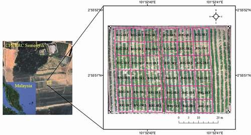
The study site was located at the Field Research Centre of Crops for the Future (CFF-FRC) in Semenyih, Malaysia (2° 57ʹ N and 101° 51ʹ E; 560 m above sea level), shown in Figure 1. The field trial was conducted from April 2018 to September 2018.

Figure 1. Study area and experimental design. Field site at the Field Research Centre of Crops for the Future in Semenyih, Malaysia. Experimental layout of plots as shown in aerial photo mosaic RGB in bird’s-eye view taken at a height of 10 meters on 22 June 2018 at flowering stage using the integrated DJI Phantom 4 Pro camera. B1G1R1 means; plot is in block 1, genotype is genotype 1 and replicate is the first replicate.

The region has a humid tropical climate with an average regional annual precipitation of 1493 mm, average annual temperature of 32.0°C, the average daily photoperiod was 12 hours and 195 rainy days. The total rainfall received at the study site during the 2018 growing season from April to September was 900 mm. The average humidity fluctuated between 83% and 88%. Soil water content was determined using a PR2 probe (Delta® Instruments, UK) at 10 cm, 20 cm, 30 cm, and 40 cm depth at weekly intervals. Irrigation was triggered when soil water content decreased to 50% plant available water capacity in the root zone. Soil analysis at the experimental site revealed that the soil type at this location was sandy clay loam with an average pH value of 5.23.

Three different Bambara groundnut genotypes namely NAV4, CIVB, and IITA-686 sourced from Africa were selected for their differences in canopy traits and physiology such as plant height, leaf pigmentation, leaf angle, leaf area, senescence rate, and yield. The three genotypes NAV4 (genotype 1), IITA-686 (genotype 2) and CIVB (genotype 3) were laid out in a randomized complete block design with four blocks, each block subdivided into nine plots and each genotype replicated three times within each block (Figure 1). For the whole trial, each genotype was replicated 12 times (4 blocks × 3 replicates per block). The total study area was 2000 m² or 0.2 ha. The gross plot size was maintained at 8 × 7 m (56 m²) while the net plot area was maintained 30 m² (6 m (length) × 5 m (width)). The row-to-row (inter-row) spacing between rows was maintained at 40 cm while plant-to-plant (intra-row) spacing was at 30 cm. There was a total of four ridges per plot. The land was ploughed, harrowed, and levelled prior to sowing; plots were demarcated and ridged at 75 cm spacing and were 30 cm high. A border row of local Bambara groundnut was grown to prevent border effect. Seeding rate was 300,000 seeds/ha of each genotype (NAV4, CIVB, IITA-686). Seeds were treated with the fungicide Dimethyldithiocarbamate before sowing. Two-seeds were sown in a hole to a depth of 3–5 cm by the dibbling method with a precision planter on 25 April 2018. Seedlings were thinned to one seedling per hill at 21 days after sowing (DAS) to give a plant density of 15 plants/m². Prior to sowing a starter fertilizer was applied at the rate of 20:60:40 nitrogen, phosphorus, and potassium (NPK) per hectare using NPK 15:15:15, triple superphosphate (46% phosphorus pentoxide), and muriate of potash (60% potassium oxide) as nutrient sources for optimal plant development. Fungicides (mancozeb 80% w/w at the rate of 2.5 kg ha⁻¹) and insecticide (cypermethrin 5.5% at the rate of 800 ml ha⁻¹) were applied at 4, 6, and 8 weeks after sowing to control fungal diseases and insects during the trial. Weeding was carried out at regular intervals by hand-hoeing.

At sowing time, each of the four corners of the field was demarcated with a square wooden frame of dimension 60 × 60 cm covered with canvas fabric and painted with weather resistant white and black paint in chequerboard design that was clearly visible in aerial imagery and distinguishable from surrounding vegetation. Each wooden frame was fixed on a polyvinyl chloride (PVC) pole at a height of 1 m above ground level at each corner of the field. These acted as permanent ground control points (GCPs). Accurate global positioning system (GPS) coordinates were collected at each of these GCPs PVC pole for later geographic registration of the captured images (Figure 1).

The average LAI in the different growth stages shows a rapid increase from vegetative (0.87 m² m⁻²) to flowering (2.57 m² m⁻²) followed by a slower increase from podding (3.75 m² m⁻²) to podfilling (4.15 m² m⁻²) reaching a maximum value in maturity (4.24 m² m⁻²) and a subsequent decline in senescence (3.99 m² m⁻²). The complete descriptive statistics are provided in the supplementary material (Table S3).

2.2. Field sampling of Bambara groundnut yield

Yield components were determined at harvest on 10 September 2018. Three samples of Bambara groundnut yield were harvested per plot by using a 1 × 1 m wooden-square frame from the centre two rows of each plot. A total of 36 samples were taken for the whole experiment. Bambara groundnut plants were manually harvested by gently pulling out of the soil and tap-roots severed at 10–15 cm using a hand hoe. After harvest, the pods were threshed, deshelled, and air-dried to constant weight in the shade. Bambara groundnut yield from each plot was determined and final seed yields were adjusted to 10% moisture content (Sesay et al. 2010). Bambara groundnut yield was recorded in tonnes/ha.

2.3. UAV, sensor, and data acquisition missions

The UAV platform used for the present study was the quadcopter Da-Jiang Innovations (DJI) Phantom 4 Pro (DJI Company, Shenzhen, China; https://www.dji.com/). This particular UAV was selected primarily because of its electric-powered, low cost, durable airframe made of titanium and magnesium, 4-direction obstacle avoidance feature, and relatively large payload bay suitable to mount any sensor. The UAV can carry a maximum payload of 477 g for 20–30 minutes with a maximum flight range is 7 km. A Canon S100 modified by MaxMax (LDP LLC, Carlstadt, NJ 07072, U.S.A., www.maxmax.com) to Green–Red-NIR (520–880 nm) was mounted on the UAV using a two-axis aluminium-carbon-fibre gimbal. The gimbal mitigated airframe vibration (pitch and roll) caused by wind and allowed pointing vertically downwards for nadir image collection. Similar low-cost UAV-camera system has been recently used for high throughput phenotyping (Duarte-Carvajalino et al. 2018; Haghighattalab et al. 2016)

The flight missions were conducted on cloudless days with clear skies at low wind speed between 10:00 h and 14:00 h local Malaysian time within ±2.0 h of solar noon. The mission was carried out under the aforementioned conditions in order to minimize variation in illumination and solar zenith angle (Haghighattalab et al. 2016). The flight duration was around 20–25 min. The flight path and settings were predetermined on the DJI Ground Station Pro (DJI GS Pro) software and the flight planning chosen was the ‘moving box’ technique. Flight altitude for each flight was set at 10 m and flight speed at 0.5 m s⁻¹. A Dell® Inspiron 7000 laptop (Dell Technologies, Round Rock, Texas, U.S.A.) installed with the ground controlling station (GCS) software was used to control and monitor the UAV flight through wireless (Wi-Fi) network.

The modified Canon S100 was set to time value (TV) mode, which enabled setting of constant shutter speed, the aperture was auto controlled by the camera to maintain a good exposure level for each flight. Canon hack development kit (CHDK) free development software kit (www.chdk.wkia.com) was used to automate the functionality of the Canon S100 in a non-destructive and non-permanent way. The CHDK script allowed the UAV autopilot system to send electronic control signals to automatically trigger the camera shutter for more refined control of data recording and for timing of the camera trigger. For the data collection flight, auto triggering was set every 3 s (frequency 0.33 Hz) thus allowing the capture of approximately 400 images for 20 min flight duration.

Flight speed and path together with sensor parameters were carefully selected to ensure that there was enough overlapping between the images for further mosaicking and to minimize pixel smearing. The sensor setting resulted in 80% forward overlap and 80% side overlap which was sufficient to generate high-quality mosaics. Prior to each flight, the modified-Canon S100 camera white balance was set by using a white card in sunlight with no filter on the camera. The captured images and GPS coordinates were recorded in a 16-bit local digital memory card in raw geographic tagged image file format (GeoTIFF) files for future post-georeferencing and mosaicking.

For ground truth validation, field reflectance measurements were taken using a FieldSpec HandHeld 2 portable spectroradiometer (ASD Inc., Longmont, CO, U.S.A.) right after each flight mission. The spectroradiometer has a spectral range of 325–1075 nm with a wavelength accuracy of ±1 nm, resolution of <3 nm at 700 nm, and a 25° circular field of view (aperture) full conical angle. The spectroradiometer was configured to average 20 readings automatically per sampling. Top-of-canopy reflectance measurements were acquired from 1 m above the canopy with the spectroradiometer in nadir view. Four Bambara groundnut plants from the centre two rows of each plot were measured 2–3 times for top-of-canopy reflectance and averaged per plot. At each phenological stage, a total of 36 spectral measurements were taken with 12 spectral measurements for each genotype. Optimization and white panel reflectance measurements were repeated every ten minutes. The averages of the VIs calculated from these spectroradiometer spectra were used for comparison with the VIs derived from the UAV imagery.

A total of six data acquisition campaigns were performed during critical crop growth period namely vegetative (41 DAS), flowering (58 DAS), podding (84 DAS), podfilling (97 DAS), maturity (105 DAS), and senescence (114 DAS) as detailed in Table 1.

Table 1. Remote sensing and proximal sensing data acquisition during Bambara groundnut growing season in 2018

Acquisition Date (d/m/y)	UAV flight missions				ASD handheld spectroradiometer
	Growth Stages	DAS	Flight altitude (m)	Total no. of images captured	GSD* (mm)	Height above canopy (m)	Number of spectra	Footprint diameter (m)
5 June 2018	Vegetative	41	10	400	4.0	1.1	36	0.5
22 June 2018	Flowering	58	10	380	4.0	1.1	36	0.5
18 July 2018	Podding	84	10	395	4.1	1.1	36	0.5
31 July 2018	Podfilling	97	10	400	4.0	1.1	36	0.5
8 August 2018	Maturity	105	10	385	4.1	1.1	36	0.5
17 August 2018	Senescence	114	10	390	4.1	1.1	36	0.5

DAS means Days After Sowing; *Ground sampling distance (GSD) was averaged for all images in a flight. Variations in GSD are due to slight fluctuations of UAV altitude in the air.

2.4. Image processing operations

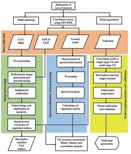
The overall workflow of the developed image processing operations is presented in Figure 2. The raw images acquired by the modified Canon S100 digital camera can have some electromagnetic contamination in the visible bands coming from the NIR band (Maxmax, LDP LLC, Carlstadt, NJ 07072, U.S.A.; www.maxmax.com). The raw images were pre-processed to completely remove NIR contamination from the red and green bands using the Remote Sensing Explorer Software Version 1.0 by MaxMax (LDP LLC, Carlstadt, NJ 07072, U.S.A.; www.maxmax.com). Further pre-processing was undertaken using the Digital Photo Professional (DPP) image processing software developed by Canon (http://www.canon.co.uk/support/camera_software/). The DPP processing included lens distortion correction, chromatic aberration, and gamma correction. White balance adjustment was achieved by using the pictures of greyscale calibration panel captured during flights. Finally, the pre-processed images were converted to the tagged image file format (TIFF) format from RAW and exported as 3-band 16-bit linear TIFF images.

Figure 2. Image processing workflow and proposed method for estimating Bambara groundnut yield using the low cost UAV imaging system.

The TIFF images were processed on the Agisoft Photoscan Pro Version 1.4.3 (Agisoft LLC St. Petersburg, Russia), where the individual images were stitched together using a structure-from-motion algorithm to generate a single high quality and high resolution orthomosaic image for the entire study area for each flight date in GeoTIFF format. The orthomosaic was then imported to ArcMap Version 10.2.2 (ArcGIS®, ESRI Inc., Redlands, AB, Canada; https://www.esri.com/en-us/arcgis/about-arcgis/overview) for geo-rectification to GCPs coordinate for each date. The GPS coordinate of the centre of the GCPs were surveyed using real-time kinematic (RTK)-enabled dual- frequency Leica 1200 Global Navigation Satellite System (GNSS) system. The study adopted the World Geodetic System WGS 84 as coordinate system.

For radiometric calibration, four 2 × 2 m horizontal calibration targets in different shades of grey having near Lambertian properties with nominal reflectance values 12%, 22%, 48%, and 80% were laid down adjacent to the study area during each flight mission and captured by the camera. The spectral reflectance of the tiles was recorded in-situ before each flight using a handheld ASD Spectroradiometer (FieldSpec, ASD, Boulder, CO, U.S.A.). For each of the flight dates, the digital number (DN) values of the calibration targets were extracted from the image using ArcMap (ArcGIS®, ESRI Inc., Redlands, AB, Canada; https://www.esri.com/en-us/arcgis/about-arcgis/overview). Linear equations using the empirical line method (Smith and Milton 1999) were developed between the calibration target DN values and the known reflectance of the calibration targets. The calibration equation developed was further used to convert the UAV imagery from DN to reflectance values for further post-processing operations.

The area of interest (AOI) was clipped from the original image using the ArcMap geoprocessing clip tool and saved as subset layer thus retaining only the relevant part of the study area. Plot quadrats were manually digitized using the ArcMap Editor tool.

Once the quadrats were digitized, masks were manually created and applied over the canopy focusing on the central portion of the canopy and excluding the border edges where mixed-pixels were prevalent. The pure canopy pixels were then used to compute average reflectance.

2.5. Calculation of VIs

After pre-processing procedures, a set of common ratio VIs previously used for grain yield prediction (Kyratzis et al. 2017; Maimaitiyiming et al. 2019; Fu et al. 2020) was calculated using the raster calculator tool in ArcMap from remotely and proximally sensed data. These include the normalized difference vegetation index  (NDVI) (Rouse et al. 1974), green normalized difference vegetation index (GNDVI) (Gitelson and Merzlyak 1998), simple ratio (SR) (Jordan 1969) and the enhanced vegetation index 2 (EVI2) (Jiang et al. 2008). The VIs were extracted quadrat-wise and the mean and standard deviation were generated using the ArcMap Zonal Statistics tool. The whole process was automated by building a model using the model builder tool in ArcMap to speed up the extraction process and facilitate date-wise extraction of VIs.

2.6. Statistical analysis and model development for yield prediction

All statistical analysis was done using STATGRAPHICS Centurion XV, version 15.2.11 (StatPoint Technologies, Warrenton, VA, U.S.A.). Initial outlier control and detection of data with divergent behaviour were carried out using the method described by Hansen et al. (Hansen, Jørgensen, and Thomsen 2002). Data normality was tested using the Kolmogorov–Smirnov test to ascertain the normal distribution. Descriptive (frequencies, means, percentages, standard deviation, and coefficient of variation (CV)) and multivariate statistics (correlation and regression analysis) were evaluated. Pearson correlation coefficients (r) were calculated between remotely-sensed indices and proximally-sensed indices. The Bland–Altman concordance test (Altman and Bland 1983) was used to evaluate the agreement of remotely-sensed indices and proximally-sensed indices. Bias and limits of agreements were calculated by computing the mean and first and third quartiles respectively. Bias was calculated as the average difference and limits of agreement were calculated as bias ± 1.96 times difference standard deviation (Bland and Altman 2010). Finally, both bias and limits were superimposed to the scatterplot. Pearson correlation coefficients between remotely sensed single-stage/multi-stage cumulative VIs and Bambara groundnut dry yield were also calculated. The cumulative VIs (∑NDVI, ∑SR, ∑GNDVI and ∑EVI2) were calculated by multiplying averaged VI values between two spectral measurements by the time interval in days (Xue, Cao, and Yang 2007; Zhou et al. 2017) as shown in Equation (1).

(1) $\sum \mathrm{V}\mathrm{I}=\underset{a}{\overset{b}{\int }}\mathrm{V}\mathrm{I}\mathrm{d}t=\sum _{i=a}^b\frac{1}{2}(x_i+x_{i+1})$(1)

where x_i represents the VI value at a particular growth stage, a and b represent days after sowing (DAS) for two growth stages.

Improved transferability and generalization of prediction models are dependent on the variability of the calibration and validation dataset (Morellos et al. 2016). Thus, to increase the transferability of the developed prediction models, care was taken to ensure that groundnut yield were representative of the various conditions. This was achieved by involving different genotypes sourced from different regions of Africa having contrasting characteristics. Moreover, the use of several genotypes to build a model adds breadth to the relationship between accumulative VIs and groundnut yield.

The best stages (integration interval) and best VIs for yield prediction were identified from the correlation results. The dataset were randomly divided into two sets: the first consisted of construction set (training), in which 75% were used to elaborate the calibration regression models; and the second one, a validation set (testing) 25%, to evaluate the yield prediction capacity of the models. Regression analyses were used to study the relationships among the dependent variable of sampled Bambara groundnut yield and the independent variable of accumulative VIs. Several models were used to analyse the relationship between yield and spectral VIs including linear function, exponential function, logarithmic function, polynomial function, and power function. The predictive power and robustness of the prediction model were determined by common evaluation metrics which include the coefficient of determination (R²) between the predicted and observed parameters, root-mean-square error (RMSE), and mean absolute performance error (MAPE). The maps for actual and predicted yield was generated using ArcGIS 10.2.2 software (ESRI Inc., Redlands, CA, U.S.A.).

3. Results

3.1. Descriptive statistics

3.1.1. Bambara groundnut yield

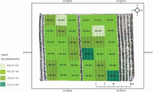
The descriptive statistics of field harvested Bambara groundnut dry seed yield is described below. The number of samples were 36. The mean Bambara groundnut dry seed yield in 2018 was 0.87 tonnes/ha. A high spatial variability with a range of 0.38–1.62 tonnes/ha was observed. The standard deviation was 0.32 tonnes/ha and CV was 36.86%. Bambara groundnut dry seed yield presented different degrees of variation as shown in Figure 3.

Figure 3. Spatial variability of Bambara groundnut yield and the productivity of different plots within one field. The value ranges of yield are presented according to the four quartiles.

3.1.2. UAV-Based VIs

During 2018 Bambara groundnut growing season, the four VIs in the six growth stages ranging from vegetative to flowering exhibited the mean values as reported in Table 2. The complete descriptive statistics are provided in the supplementary material (Table S1). It can be seen that the mean values of all indices were lowest during the vegetative stage. Mean values of NDVI, EVI2, and GNDVI gradually increased and reached their peaks during the podding stage except for SR which staged higher mean value at podfilling stage. Podding is characterized by a mature canopy with very high photosynthetic rate and the onset of underground pods. The mean values remain almost the same from podding to maturity. After maturity, the mean values decreased indicating the onset of senescence characterized by the progressive yellowing of leaves and degradation of leaf pigments. Mean and median values never diverged by more than 5%. The highest divergence observed was 4.5% for EVI2 at senescence stage. VIs CV was more contained than yield variation. Average CV was 9.1%, and highest CV was 22.0%. NDVI and GNDVI had the lowest CV averaging 5.1% and 5.8%, respectively, for all the different growth stages while SR and EVI2 had the highest CV averaging 10.9% and 14.6%, respectively. There was a general trend of increase in CV from flowering to senescence. Lastly, data was normally distributed (non-significant Kolmogorov–Smirnov test in all cases). The standardized skewness and standardized kurtosis are within the range (−2 to +2) expected for data from a normal distribution (Table S1).

Table 2. Descriptive statistics of the UAV based spectral VIs at different crop stages for 2018 Bambara groundnut growing season

Growth Stages	NDVI			EVI2			SR			GNDVI
	Mean ± SD	Range	CV (%)	Mean ± SD	Range	CV (%)	Mean ± SD	Range	CV (%)	Mean ± SD	Range	CV (%)
Vegetative	0.56 ± 0.03	0.50–0.62	5.2	0.24 ± 0.05	0.13–0.35	22.0	2.25 ± 0.10	2.09–2.50	4.2	0.47 ± 0.03	0.43–0.51	5.3
Flowering	0.75 ± 0.03	0.70–0.80	4.2	0.65 ± 0.08	0.53–0.77	11.6	3.86 ± 0.39	3.12–4.44	10.2	0.58 ± 0.03	0.54–0.63	5.3
Podding	0.80 ± 0.04	0.73–0.85	4.8	0.74 ± 0.09	0.59–0.88	12.5	4.07 ± 0.47	3.25–4.71	11.6	0.60 ± 0.03	0.55–0.64	5.4
Podfilling	0.78 ± 0.04	0.72–0.83	5.1	0.73 ± 0.09	0.59–0.85	12.0	4.25 ± 0.56	3.41–5.06	13.2	0.60 ± 0.04	0.54–0.65	6.5
Maturity	0.80 ± 0.04	0.73–0.85	5.0	0.74 ± 0.09	0.60–0.87	12.7	4.25 ± 0.45	3.51–4.80	10.7	0.59 ± 0.03	0.54–0.63	5.0
Senescence	0.76 ± 0.05	0.68–0.82	6.3	0.67 ± 0.11	0.50–0.81	16.9	3.70 ± 0.57	2.92–4.56	15.3	0.56 ± 0.04	0.50–0.62	7.5

SD: standard deviation; CV: coefficient of variation; Kolmogorov–Smirnov test is non-significant for all indices at each growth stages.

3.2. Comparison between VIs derived from remote sensing and proximal sensing

The average plot VIs obtained from remote sensing and proximal sensing were all highly and significantly (P < 0.01) correlated with each other (Table 3). To test the accuracy of the indices derived from UAV based Canon S100 by comparison with the ASD spectroradiometer, we calculated the band equivalent reflectance (BER) for the Canon S100. This was done by taking the average of all the spectroradiometer bands that are within the full width at half maximum of the camera. The correlation coefficients for the same VIs remotely vs. proximally sensed were above 0.77 (r > 0.77, P < 0.01) for all the VIs. Among all the VIs calculated for the Canon S100, NDVI had the highest correlation (r = 0.88, P < 0.01) with the spectroradiometer followed by EVI2 (r = 0.85, P < 0.01), SR (r = 0.84, P < 0.01) and GNDVI having the lowest correlation (r = 0.78, P < 0.01). High correlation coefficients were observed between VIs extracted from the spectroradiometer and from the Canon S100. This indicates the suitability of the VIs derived from the modified near-infrared sensitive digital camera for PA. Factors such as low flight altitude and low flying speed may have played a role in the high correlation observed between measurements from UAV based Canon S100 with the ground truth measurements. VIs derived from the UAV platform had higher CV compared to the VIs derived from the ground-based spectroradiometer (Tables S1 and S2).

Table 3. Correlation coefficients between VIs extracted from remote sensing UAV imagery data (UAV) and proximal sensing BER values derived from data acquired by the spectroradiometer (gt)

	NDVIUAV	EVI2UAV	SRUAV	GNDVIUAV
NDVIgt	0.88**	0.87**	0.78**	0.73**
EVI2gt	0.85**	0.85**	0.77**	0.71**
SRgt	0.77**	0.79**	0.84**	0.75**
GNDVIgt	0.82**	0.83**	0.78**	0.78**

**Correlation is significant at the P < 0.01 level (2-tailed).

Scatterplots (Figure 4) show the linear relationship between VIs derived from UAV and VIs derived from groundtruthing as confirmed with a test of normality of residuals of the linear models. For all the VIs pairs, the null hypothesis could not be rejected (P > 0.95). For all VIs pairs, analysis of variance (ANOVA) tests indicate a significant relationship (P < 0.05) between the indices from UAV and indices from groundtruthing at the 95% confidence level. In all cases, the correlation coefficients were greater than 0.77 thus indicating a moderately strong relationship between the variables. The observed RMSE values were very low in all cases ranging from 0.03 for GNDVI to 0.46 for SR.

Figure 4. Scatterplots indicate the linear relationship between the indices derived from data acquired by Canon S100 and BER indices derived from data acquired by spectroradiometer; (a) NDVI, (b) EVI2, (c) SR, and (d) GNDVI.

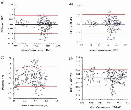
Figure 5 shows the results of the Bland–Altman plot comparing remotely-sensed indices and proximally-sensed indices. For NDVI, the estimated difference was low, at −0.005. The upper limit of agreement was 0.090 and the lower limit of agreement was −0.101. For EVI2, the estimated difference was low, at −0.013. The upper limit of agreement was 0.209 and the lower limit of agreement was −0.234. For SR, the estimated difference was low, at 0.155. The upper limit of agreement was 1.122 and the lower limit of agreement was −0.811. With regards to GNDVI, the estimated difference was low, at 0.006. The upper limit of agreement was 0.085 and the lower limit of agreement was −0.073. All the measurements occurred within two standard deviations of the mean difference. In all cases, most of the values lie within the limits, which indicates that there is a strong agreement between the two quantitative measurements of indices.

Figure 5. Bland–Altman plots comparing VIs calculated from data acquired by UAV based Canon S100 multispectral images and BER indices derived from data acquired by Spectroradiometer; (a) NDVI, (b) EVI2, (c) SR, and (d) GNDVI. Blue dots are individual random samples; black solid lines indicate mean bias and red solid lines indicate the upper and lower limits of agreement.

3.3. Determination of the optimum single growth stages and best spectral VIs for yield prediction

3.3.1. Correlations between VIs and Bambara groundnut yield at different growth stages

The relationship between Bambara groundnut yield and the four VIs at different growth stages were analysed using the datasets (Table 4). The results show a weak positive correlation (P < 0.05) between yield and NDVI, EVI2, and SR at vegetative stage. However, no significant correlation was observed between yield and GNDVI at the vegetative stage. A moderate positive correlation (P < 0.01) was observed between yield and all the VIs except GNDVI, which was significant at P < 0.05. A strong positive correlation exceeding (r > 0.60, P < 0.01) was observed between all the VIs and yield at the podding, podfilling and maturity stages. Results indicate that these stages are highly correlated with yield. The maximum correlation coefficient achieved was at podfilling stage. The maximum value of the correlation was (r = 0.81, P < 0.01) with SR. Thus, the podfilling stage was the best growth stage for estimation of Bambara groundnut yield using spectral VIs. The magnitude of the correlation decreased from maturity to senescence stage. Moderate positive correlation coefficients (P < 0.05) were observed between yield and the spectral VIs at senescence stage. The least performing stages for yield prediction were the vegetative, flowering and senescence stage with the minimum correlation occurring at the vegetative stage. Overall, over the whole growth period, SR and NDVI performed best followed by EVI2 and GNDVI.

Table 4. Pearson correlation coefficients between Bambara groundnut dry seed yield and spectral VIs at different growth stages

Growth stage	Spectral VIs
	NDVI	EVI2	SR	GNDVI
Vegetative	0.37*	0.36*	0.38*	0.32
Flowering	0.46**	0.45**	0.48**	0.40*
Podding	0.71**	0.67**	0.72**	0.63**
Podfilling	0.80**	0.78**	0.81**	0.77**
Maturity	0.75**	0.71**	0.75**	0.71**
Senescence	0.49**	0.45**	0.51**	0.43**

**Correlation is significant at the P < 0.01 level (2-tailed); *Correlation is significant at the P < 0.05 level (2-tailed); NIR, R and G represents the NIR, red and green bands, respectively.

3.3.2. Correlations between accumulated spectral VIs and Bambara groundnut yield at various growth stages

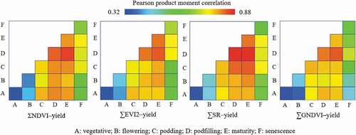
Further analysis was conducted on the relationship between Bambara groundnut yield and cumulative multi-temporal spectral VIs. Figure 6 shows the relationships between Bambara groundnut yield and cumulative spectral VIs. The cell values in the correlogram indicate the Pearson correlation coefficient between yield and the accumulated spectral VIs from the vegetative stage to the senescence stage. The results show that the correlation between yield and cumulative spectral indices increase corresponding to the increase in the cumulative spectral indices by growth stages, from vegetative stage to maturity stage. Thereafter, there is a decrease in the magnitude of the correlation. The result indicates that accumulated spectral VIs from podfilling to maturity stage contains a large volume of crop growth biophysical data, thus reflecting a biological impact of plant growth status on Bambara groundnut yield. The best performance observed was from podfilling to maturity. The highest correlation coefficient was achieved between yield and ∑SR from podfilling to maturity stage (r = 0.88, P < 0.01). ∑NDVI from podfilling to maturity stage also exhibited high correlation coefficient with yield (r = 0.87, P < 0.01). Both ∑EVI2 and ∑GNDVI exhibited poorer correlations with yield and were excluded from further analysis. The correlation between yield and cumulative indices decreased from maturity stage to senescence stage.

Figure 6. Correlation of Bambara groundnut yield with the cumulative VIs from vegetative stage to senescence stage.

3.4. Establishment and validation of yield prediction model

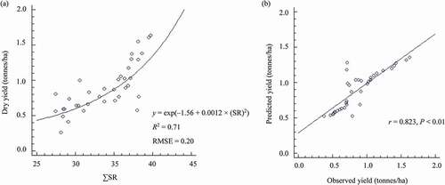
According to the above results, SR (r = 0.81, P < 0.01) and NDVI (r = 0.80, P < 0.01) at the podfilling stage and ∑SR (r = 0.88, P < 0.01) and ∑NDVI (r = 0.87, P < 0.01) from podfilling stage to maturity stage exhibited good correlations with Bambara groundnut yield. Table 5 shows the result of the regression analysis between yield and both single stage VIs and accumulated multi-temporal VIs. Results indicate that the model with cumulative spectral indices had higher coefficient of determination than the single stage spectral indices. The model with accumulated spectral indices exhibited more stable performance with lower RMSE and lower MAPE when compared to model based on single stage spectral indices. The best model was based on ∑SR from podfilling to maturity stage which exhibited a good exponential relationship with yield (R² = 0.71, RMSE = 0.20, MAPE = 14.2%) (Figure 7(a)). Furthermore, high correlation of (r = 0.82, P < 0.01) was observed between predicted yield versus observed yield (Figure 7(b)). The results indicate that ∑SR from podfilling stage to maturity stage better represented the intensity and photosynthetic activity of the crop and outperforms single stage spectral VIs in reliably predicting Bambara groundnut yield for the growing season.

Table 5. Quantitative relationships between yield (y) and spectral VIs (x) in Bambara groundnut for 2018 growing season

Spectral vegetation index	Growth stage	Model calibration		Model validation
		Fitting model	R^2	RMSE	MAPE (%)
SR	Podfilling	y = exp(−1.37 + 0.064 × (SR)^2)	0.68	0.24	15.1
NDVI	Podfilling	y = exp(−5.97 + 7.40 × NDVI)	0.66	0.21	14.7
∑SR	Podfilling to maturity	y = exp(−1.56 + 0.0012 × (SR)^2)	0.71	0.20	14.2
∑NDVI	Podfilling to maturity	y = 1/(16.3–8.15 × ln(NDVI))	0.70	0.22	14.5

Figure 7. (a) Relationship between yield and ∑SR from podfilling to maturity stage; (b) Correlation between predicted field-scale yield estimated by regression model developed and observed field yield using independent validation (test) data set.

Table 6 describes the comparison between predicted dry seed yield and observed dry seed yield of the entire field after applying the empirical yield prediction equation to the whole field’s pixels. The average observed dry seed yield was 0.87 tonnes/ha while the average predicted dry yield was 0.90 tonnes/ha. The prediction error was described as results of comparing the total observed yield versus the total predicted yield. The prediction error was low at 13.9%. This high prediction accuracy can be attributed to accurate VIs value obtained from high resolution multispectral images captured by the UAV platform, which enabled the effective spectral separation of healthy vegetation from non-vegetated areas so that noise from soil and background was completely removed.

Table 6. Predicted yield versus observed yield for the growing season

	Predicted dry seed yield (tonnes/ha)	Observed dry seed yield (tonnes/ha)
Min yield	0.53	0.38
Max yield	1.36	1.62
Average yield	0.90	0.87
Standard error	0.05	0.05
Standard deviation	0.27	0.32
Prediction error (%)	13.9

3.5. Spatial yield prediction of Bambara groundnut

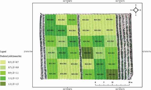
The yield prediction map of the study area was generated in ArcMap using the empirical formula developed for yield prediction y = exp(–1.56 + 0.0012 × (SR)²). From the map, within-field spatial variations of yield could be better understood for PA operations such as site-specific or variable-rate fertilizer applications. The map produced showed considerable variation in within-field yield as represented by the distinct five productivity classes represented by colour symbology as shown in Figure 8. The estimated average yield of the study site was 0.90 tonnes/ha. A low yield could be observed across the field borders and boundaries. From the Bambara groundnut yield map we found out that 5.6% of the area had very high productivity of 1.3–1.5 tonnes/ha; 25.0% of the area had high productivity of 1.1–1.3 tonnes/ha, 22.2% of the area had medium productivity of 0.9–1.1 tonnes/ha, 11.1% of the area had low productivity of 0.7–0.9 tonnes/ha and 36.1% of the area had very low productivity of 0.5–0.7 tonnes/ha.

Figure 8. Map of predicted Bambara groundnut yield expressed as dry seed weight in tonnes/ha.

4. Discussion

Bambara groundnut is an indeterminate legume capable to meet its nitrogen requirement throughout its growth stages by nitrogen fixation therefore nitrogen fertilization is not necessary and can sometimes have negative effect on plant growth and even lead to reduced seed yields (Wessel, Keltjens, and Cleef 2012). Starter fertilizer applied prior to sowing stimulate root growth and root nodulation in leguminous plants (Wafula et al. 2021) and does not have any significant effect on Bambara groundnut growth and yield at harvest (Wessel, Keltjens, and Cleef 2012). Thus, the starter fertilizer did not have any effect on the high/low vigour of the crop over different stages. The observed high/low vigour is associated with vegetation productivity, biomass production, high chlorophyll content and canopy growth status (Onyia, Balzter, and Berrio 2018). The yield of Bambara groundnut in Malaysia varies between landraces and locations (0.50–3.0 tonnes/ha) with an average yield of 0.85 tonnes/ha (Musa et al. 2016; Suhairi, Jahanshiri, and Nizar 2018). In this study, the observed mean Bambara groundnut dry seed yield for the 2018 growing season showed a high variability ranging from 0.38–1.62 tonnes/ha with a mean of 0.87 tonnes/ha (CV = 36.6%) (Figure 3). The CV denotes a high yield variation greater than the 20% threshold thus indicating high variation in field attributes (Ali et al. 2019). This was a favourable circumstance in this study allowing us to test the suitability of the VIs to predict yield under conditions of high spatial variability.

The temporal dynamics of the four studied UAV based multispectral VIs in the six different phenological stages are shown in Table 2. The mean values of the VIs were lowest during the vegetative stage. This is because at the vegetative stage, the Bambara groundnut canopy was not fully developed and fractional vegetation cover was very low. When the plants are small, soil background reflectance is very high. Angular VIs such as NDVI and SR are very sensitive to the soil effect and might not perform well at low LAI values, at relatively sparse vegetation cover (Liu, Pattey, and Guillaume 2012; Broge and Leblanc 2001). The values of the VIs increase from vegetative stage and reaches maximum at podding stage as the canopy develops. The high value of the VIs observed indicates healthy and well growing crops. However, high VIs do not necessarily indicate higher Bambara groundnut yield since higher aboveground biomass contributes to high vigour canopies and is not a prerequisite for higher yield (Ali et al. 2019). From podding to maturity, the values of the VIs do not fluctuate much as the indices gets saturated as the LAI increases and reached a value of 4 and then remain high until maturity, as reported previously (Hatfield and Prueger 2010). Variations in the canopy reflectance begins to decline afterwards until the senescence stage; this behaviour is due to crop senescence characterized by degradation of chlorophyll pigments and defoliation (Hussain et al. 2020; Din et al. 2017). Similar pattern of changes in VIs in different phenological stages collected over corn (Zea mays L.), canola (Brassica napus L.), soybean (Glycine max L.), and wheat (Triticum aestivum L.) canopies was observed by other researchers (Hatfield and Prueger 2010; Ali et al. 2019). The VIs variation was more contained (CV = 9.1%) than yield variation (CV = 36.86%) indicating that there was very low range of variability in acquired VIs. Among the VIs, NDVI and GNDVI showed the best performance with a CV lower than 10%. This can be attributed to the fact that they are normalized indices (Gianquinto et al. 2019). The data of both yield and UAV-based VIs were normally distributed (non-significant Kolmogorov-Smirnov test), which is a prerequisite for regression models (Paul and Zhang 2010).

We found that VIs extracted from the spectroradiometer and the UAV-based Canon S100 camera were highly-correlated with each other (r > 0.77, P < 0.01) for all the VIs (Table 3) in the same order of magnitude as the correlation between proximally and remote-sensed indices (r > 0.75, P < 0.01) reported by Di Gennaro et al. (2018). Haghighattalab et al. (2016) found good correlation (r = 0.76, P < 0.05) between VIs derived from the spectroradiometer and VIs from a calibrated Canon S100 camera. Tattaris, Reynolds, and Chapman (2016) and Primicerio et al. (2012) reported similar strong correlations between airborne NDVI and equivalent ground-based NDVI (r = 0.78, P < 0.01) (r = 0.97, P < 0.01), respectively. However, correlations between the derived indices from UAV based modified digital cameras and the derived indices from the high resolution spectroradiometers must be treated with caution.

As the ground and aerial measurements were taken at the same time on the same day, variation in environmental conditions such as light intensity and brightness were almost negligible. Moreover, platform movements were minimal due to favourable environmental conditions, low flying altitude and high stability of the camera gimbals. Thus, the main factor affecting correlation of proximally and remotely sensed VIs were due to the resolution of the sensors. When spatial resolution is high, reflectance captured are mostly from vegetation; however, when the spatial resolution is lower, the boundaries between vegetation and non-vegetation such as soil are fuzzy thus the reflectance might include information from both plants and soil. Indeed, high spatial resolution images captured by low altitude flying UAV have favourable signal-to-noise ratio thus allowing the effective elimination of shadow and soil pixels with high confidence. The relative precision of the airborne measurements can thus be attributed to two main factors. First, the effective radiometric calibration and effective removal of non-vegetated pixels and other outliers during image analysis. Second, through the thorough limitation of the confounding effects caused by environmental drift such as changes in temperature, sun angle etc. typically associated with time taken to make ground based measurements. With regards to field spectroscopy measurements, care was taken to ensure the field of view (FOV) of the spectrometer covered the canopy thus reducing background effects (e.g. soil). Moreover, data pre-processing procedures such as filters were used to smooth noise and to average spectra to further reduce errors. The ground sampling represents a much smaller area. Thus, the measurements captured englobes more specific small-size spectral features within the cylindrical footprint area. The captured spectral signatures might be from healthy leaves, unhealthy leaves or even leaves with varying portion of shadows (Gautam et al. 2020). To account for the very small field of view of the spectroradiometer, we constantly monitored the spectral response curves to avoid mixed pixels thus contamination in our samples and we averaged several reflectance readings per plot. The abovementioned measures were taken to reduce the discrepancies in the remotely and proximally sensed reflectance.

Hence, the high correlations observed between remotely and proximally sensed VIs demonstrate the applicability of this low budget modified digital camera for yield prediction.

The Bland–Altman plots also indicated that there was a strong agreement between the VIs derived from proximal sensing and the VIs derived from remote sensing (Figure 5). Cogato et al. (2019) used the Bland–Altman concordance test to successfully compare NDVI extracted from Worldview-2 and Sentinel-2 images. We obtained a good agreement between the two different quantitative measurements of VIs as suggested by the correlation coefficients, the Bland–Altman plots, and the low RMSE from the scatterplots (Figure 4). Results suggest the suitability of using indices derived from a low-cost modified near infrared sensitive digital camera mounted on commercial UAV for PA applications.

In this study, the relationships between Bambara groundnut yield and spectral VIs from the multispectral images were analysed at the different growth stages. Results showed that except for GNDVI at vegetative stage, significant and positive correlations were observed between the yield and the four VIs at all growth stages studied (Table 4), thus indicating that yield can be estimated using single stage VIs acquired well in advance of harvest. Similar results were reported by other researchers (Zhou et al. 2017; Xue, Cao, and Yang 2007; Aparicio et al. 2002). Weak positive but significant correlations were observed between yield and SR, NDVI and EVI2 at the vegetative stage while GNDVI was non-significant. At the vegetative stage, the vegetation cover fraction was low with low LAI, thus the canopy reflectance was highly influenced by the strong background reflectance from dry soil, wet soil, and water surfaces that could negatively affect the performance of the red based VIs (Hashimoto et al. 2019; Walsh et al. 2018). Barati et al. (2011) reported that SR, NDVI and Infrared Percentage Vegetation Index (IPVI) are the most sensitive to low vegetation cover fraction while green indices such as GNDVI, Transformed Vegetation Index (TVI), Modified Triangular Vegetation Index 1 (MTVI1), Modified Triangular Vegetation Index 2 (MTVI2), Chlorophyll Index (CI), and Normalized Canopy Index (NCI) are the least sensitive. This is in agreement with the observed non-significant yield and GNDVI correlation at vegetative stage. However, the result is not consistent with the result obtained by other researchers that proved VIs containing the green band were better yield predictors than those including the red band (Xue, Cao, and Yang 2007; Haboudane et al. 2004). The magnitude of the correlation coefficient between yield and spectral VIs increased progressively from vegetative to podding stage as the canopy develops and there is an increase in LAI. The coefficient of correlation was highest for the spectral reflectance measured at podfilling stage for all the indices with a maximum correlation coefficient of (r = 0.81, P < 0.01) between the SR VI and yield. From podding to maturity the magnitude of the correlation coefficient did not vary much since the canopy is fully developed. This might be because crop maturity causes an increase in the visible reflectance and alteration in the NIR reflectance (Kayad et al. 2016). Another reason could be the saturation of the VIs. NDVI and SR are particularly sensitive at low LAI values between 0 and 2 typically observed at early growth stages with sparse canopies or under stress conditions (Aparicio et al. 2000). With LAI >3, addition of more canopy layers does not significantly affect the relative interceptance or reflectance of the red and near infrared radiation, thus there is little effect on the VIs (Aparicio et al. 2000). NDVI tends to saturate more easily with increasing LAI than SR and EVI2 therefore the latter two indices are more suited to study crop growth. EVI2 was intermediate between SR and NDVI in terms of variation and saturation (Hashimoto et al. 2019). Aparicio et al. (2000) showed that SR assumes a linear relationship with LAI while the relationship between NDVI and LAI is exponential for the same LAI values. Kang et al. (2016) reported that EVI/EVI2 performed best among five tested indices including NDVI, SR, EVI, EVI2, and SR in mapping large-scale global LAI. Our results confirmed their findings. From maturity to senescence stage there is a decrease in the magnitude of the correlation observed which might be attributed to senescence characterized by degradation of chlorophyll pigment, lower biomass and low LAI (Hassan et al. 2019). Indices related to LAI may not correlate as strongly with Bambara groundnut yield since there is significant foliage loss at senescence stage (Fernández, Gorchs, and Serrano 2019).

Results showed that simple ratio VI correlated better with yield compared to other VIs (Table 4). Zhao et al. (2007) reported that among SR, NDVI, EVI, and Wide Dynamic Range Vegetation Index (WDRV), SR correlated best with lint yield. Serrano, Filella, and Pen˜uelas (2000) observed significant correlations between SR and chlorophyll a pigment. Moreover, VIs calculated from the NIR and red band perform better with vegetation growth traits as opposed to GNDVI, which have lower performance due to the absence of the red band. Kyratzis et al. (2017) found that GNDVI had better discriminating efficiency and was a better predictor of yield at early reproductive stages of durum wheat grown under heat stressed environments. In this study, GNDVI performance for yield prediction was lower, which can also be explained by different environmental conditions. The lower performance of EVI2 for yield prediction may be explained by the choice of coefficient in the equation. Shi et al. (2016) and Jurecka et al. (2016) also reported EVI2 to have weaker correlations with crop yield as compared to NDVI and SR. Aparicio et al. (2002) also reported that among three VIs tested namely SR, NDVI and Photochemical Reflectance Index (PRI) for determining durum wheat yield, the simple ratio (SR) VI performed best. They also reported that SR correlated better with crop growth including photosynthetic area, biomass and grain yield as compared to NDVI. They explained that the saturation of the NDVI as opposed to SR may alter its performance in yield prediction. SR is less affected by the saturation effect of LAI greater than 3 as opposed to NDVI. Our results corroborated with their findings.

The correlogram of accumulated multi-temporal spectral VIs with yield showed that podfilling to maturity was the best integral interval to predict yield yet all were highly significant (Figure 6). Compared with VIs at the best single stage (podfilling), cumulative VIs improved the relation with yield, and ∑SR from podfilling to maturity stage was the best ∑VI, with r improving from (r = 0.81, P < 0.01) to (r = 0.88, P < 0.01). ∑NDVI from podfilling to maturity also exhibited good correlations with yield (r = 0.87, P < 0.01). Previous studies have indicated that accumulative VIs can improve the stability of yield prediction (Du et al. 2017; Wang et al. 2014). Wang et al. (2014) reported that cumulative spectral indices gives a higher prediction accuracy for wheat grain yield and protein content rather than at a single growth stage. Cumulative SR is a good indicator of crop growth as has been shown previously for a variety of crops and growing conditions (Moran, Inoue, and Barnes 1997). Serrano, Filella, and Pen˜uelas (2000) also reported that ∑SR to be a good predicator of winter wheat grain yield under different nitrogen supplies. They explained that ∑SR better tracked the duration and intensity of the canopy photosynthetic capacity and probably better reflect the contribution of the photosynthetic organs than other VIs.

Regression analysis for yield versus ∑SR and ∑NDVI from podfilling to maturity stage showed that the exponential and logarithmic form respectively was the best (R² = 0.71 for ∑SR and R² = 0.70 for ∑NDVI) (Table 5 and Figure 7). The coefficient of determination (R²) for the model based on multi-temporal VIs was higher than the models based on single stage VIs. Moreover, the values of RMSE and MAPE showed obvious differences with the models based on multi-temporal VIs exhibiting lower RMSE and MAPE values than the models based on single stage VIs thus implying that the former was more stable in yield prediction. The prediction error was low at 13.9% indicating that yield can be accurately predicted based on accumulative remote sensing data (Table 6). Previous researchers have proved that accumulative VIs can improve the stability of yield prediction models (Xue, Cao, and Yang 2007; Wang et al. 2014). Ren et al. (2008) showed that ∑NDVI from booting to flowering stage rather than single stage exhibited higher performance with better stability for the prediction of winter-wheat grain yield. Based on our findings, it appears that multi-temporal remote sensing data can provide more useful information and is more reasonable and scientific than single stage remote sensing data for yield prediction. However, when it is difficult to acquire multi-temporal remote sensing images, single stage remote sensing images appears to be adequate for early yield prediction.

Considerable spatial variation of Bambara groundnut yield thus productivity was observed throughout the field (Figure 8). Identifying the low, medium and high yield areas within the field and their temporal variation across multiple seasons will enable targeted management practices, which will increase profitability (Zhao et al. 2020). Al-Gaadi et al. (2016) observed similar patterns in productivity in three potato fields with some high-yielding areas producing an average yield of 40 tonnes/ha and some low-yielding areas producing an average yield of 21 tonnes/ha. Similar within field spatial variations in wheat yield was observed by Du et al. (2017). They reported that this was closely linked with soil fertility, water potential, and tiller density, and farmers could use the map for future variable rate fertilizer application operations.

Future research work includes testing the yield prediction model with multi-year datasets. Other crop biophysical parameters such as LAI, canopy chlorophyll content, fractional vegetation cover, aboveground biomass together with environmental data could be further analyzed to incorporate into the yield prediction model to potentially improve the accuracy of yield prediction. Moreover, effects of environment, management practices, and genotype on yield can be realized by integrating remote sensing data into crop growth models (Doraiswamy et al. 2004).

5. Conclusions

VIs derived from high resolution images acquired using a commercial UAV equipped with a modified near-infrared sensitive consumer-grade digital camera can be used to accurately predict Bambara groundnut yield and map its spatial variability. The current study reports promising correlations between remotely and proximally derived VIs. The comparison between the proximally and remotely derived indices show a good agreement between the two datasets. Based on the systematic analysis of the quantitative relationships between yield and VIs at various growth stages, the podfilling stage was identified as the best stage for estimating yield. The use of SR at podfilling stage provided a reliable estimation of yield than at any other stage. Yield could be estimated before harvest especially using VIs that include the red and near infrared band such as SR and NDVI. Cumulative spectral indices proved to be robust yield estimators, with significant results achieved by accumulating VIs from the podfilling stage to the maturity stage. The prediction model based on multi-temporal remote sensing data had increased performance and stability compared to the model based on single stage remote sensing data. The accumulated spectral VI ∑SR from podfilling stage to maturity stage is recommended for reliably estimating yield. The prediction map of within-field spatial variation in yield can help farmers and decision makers to utilize PA and optimization techniques such as variable rate applications to optimize inputs and maximize yield.

Acknowledgements

The authors thank Crops for the Future (CFF) for providing the experimental site to conduct the trial. We would like to thank DKSH Technology Malaysia Sdn Bhd for generously providing the FieldSpec HandHeld 2 portable spectroradiometer (ASD Inc., Longmont, CO, U.S.A.) for the trial.

Disclosure statement

No potential conflict of interest was reported by the author(s).

Data availability statement

The data that support the findings of this study are available from the corresponding author, [A.S.], upon reasonable request by e-mail: [email protected].

Supplementary material

Supplemental data for this article can be accessed here.

Additional information

Funding

This work was supported by the School of Biosciences of The University of Nottingham and The University of Adelaide Dual/Joint PhD Research Accelerator Award (SoB UoN-UoA RAA) under Grant [P0021.54.04].

References

- Al-Gaadi, K. A., A. A. Hassaballa, E. Tola, A. G. Kayad, R. Madugundu, B. Alblewi, and F. Assiri. 2016. “Prediction of Potato Crop Yield Using Precision Agriculture Techniques.” PLOS ONE 11: e0162219. doi:https://doi.org/10.1371/journal.pone.0162219.
- Ali, A., R. Martelli, F. Lupia, and L. Barbanti. 2019. “Assessing Multiple Years’ Spatial Variability of Crop Yields Using Satellite Vegetation Indices.” Remote Sensing 11 (20): 2384. MDPI AG. doi:https://doi.org/10.3390/rs11202384.
- Altman, D. G., and J. M. Bland. 1983. “Measurement in Medicine: The Analysis of Method Comparison Studies.” Journal of the Royal Statistical Society. Series D (The Statistician) 32. John Wiley & Sons, Ltd: 307–317. doi:https://doi.org/10.2307/2987937.
- Aparicio, N., D. Villegas, J. Casadesus, J. L. Araus, and C. Royo. 2000. “Spectral Vegetation Indices as Nondestructive Tools for Determining Durum Wheat Yield.” Agronomy Journal 92 (1): 83–91. John Wiley & Sons, Ltd. doi:https://doi.org/10.2134/agronj2000.92183x.
- Aparicio, N., D. Villegas, J. L. Araus, J. Casadesús, and C. Royo. 2002. “Relationship between Growth Traits and Spectral Vegetation Indices in Durum Wheat.” Crop Science 42 (5): 1547. Crop Science Society of America. doi:https://doi.org/10.2135/cropsci2002.1547.
- Araus, J. L., and J. E. Cairns. 2014. “Field High-Throughput Phenotyping: The New Crop Breeding Frontier.” Trends in Plant Science 19 (1): 52–61. Elsevier Current Trends. doi:https://doi.org/10.1016/J.TPLANTS.2013.09.008.
- Barati, S., B. Rayegani, M. Saati, A. Sharifi, and M. Nasri. 2011. “Comparison the Accuracies of Different Spectral Indices for Estimation of Vegetation Cover Fraction in Sparse Vegetated Areas.” Egyptian Journal of Remote Sensing and Space Science 14 (1): 49–56. Elsevier B.V. doi:https://doi.org/10.1016/j.ejrs.2011.06.001.
- Berra, E. F., R. Gaulton, and S. Barr. 2017. “Commercial Off-the-Shelf Digital Cameras on Unmanned Aerial Vehicles for Multitemporal Monitoring of Vegetation Reflectance and NDVI.” IEEE Transactions on Geoscience and Remote Sensing 55 (9): 4878–4886. doi:https://doi.org/10.1109/TGRS.2017.2655365.
- Bland, J. M., and D. G. Altman. 2010. “Statistical Methods for Assessing Agreement between Two Methods of Clinical Measurement.” International Journal of Nursing Studies 47 (8): 931–936. Pergamon. doi:https://doi.org/10.1016/j.ijnurstu.2009.10.001.
- Broge, N. H., and E. Leblanc. 2001. “Comparing Prediction Power and Stability of Broadband and Hyperspectral Vegetation Indices for Estimation of Green Leaf Area Index and Canopy Chlorophyll Density.” Remote Sensing of Environment 76 (2): 156–172. doi:https://doi.org/10.1016/S0034-4257(00)00197-8.
- Clevers, J. G. P. W. 1989. “Application of a Weighted Infrared-Red Vegetation Index for Estimating Leaf Area Index by Correcting for Soil Moisture.” Remote Sensing of Environment 29 (1): 25–37. Elsevier. doi:https://doi.org/10.1016/0034-4257(89)90076-X.
- Cogato, A., V. Pagay, F. Marinello, F. Meggio, P. Grace, and M. De Antoni Migliorati. 2019. “Assessing the Feasibility of Using Sentinel-2 Imagery to Quantify the Impact of Heatwaves on Irrigated Vineyards.” Remote Sensing 11 (23): 2869. MDPI AG. doi:https://doi.org/10.3390/rs11232869.
- Daughtry, C. S. T., K. P. Gallo, and M. E. Bauer. 1983. “Spectral Estimates of Solar Radiation Intercepted by Corn Canopies.” Purdue University, LARS Technical Report 030182 (3): 527–531. American Society of Agronomy. doi:https://doi.org/10.2134/agronj1983.00021962007500030026x.
- Deng, L., Z. Mao, X. Li, Z. Hu, F. Duan, and Y. Yan. 2018. “UAV-Based Multispectral Remote Sensing for Precision Agriculture: A Comparison between Different Cameras.” ISPRS Journal of Photogrammetry and Remote Sensing 146: 124–136. December. Elsevier. doi:https://doi.org/10.1016/J.ISPRSJPRS.2018.09.008.
- Di Gennaro, S. F., F. Rizza, F. W. Badeck, A. Berton, S. Delbono, B. Gioli, P. Toscano, A. Zaldei, and A. Matese. 2018. “UAV-Based High-Throughput Phenotyping to Discriminate Barley Vigour with Visible and near-Infrared Vegetation Indices.” International Journal of Remote Sensing 39 (15–16): 5330–5344. Taylor and Francis Ltd. doi:https://doi.org/10.1080/01431161.2017.1395974.
- Din, M., W. Zheng, M. Rashid, S. Wang, and Z. Shi. 2017. “Evaluating Hyperspectral Vegetation Indices for Leaf Area Index Estimation of Oryza Sativa L. at Diverse Phenological Stages.” Frontiers in Plant Science 8: 820. May. Frontiers Media S.A. doi:https://doi.org/10.3389/fpls.2017.00820.
- Doraiswamy, P. C., J. L. Hatfield, T. J. Jackson, B. Akhmedov, J. Prueger, and A. Stern. 2004. “Crop Condition and Yield Simulations Using Landsat and MODIS.” Remote Sensing of Environment 92: 548–559. doi:https://doi.org/10.1016/j.rse.2004.05.017.
- Du, M., N. Noguchi, M. Du, and N. Noguchi. 2017. “Monitoring of Wheat Growth Status and Mapping of Wheat Yield’s within-Field Spatial Variations Using Color Images Acquired from UAV-Camera System.” Remote Sensing 9 (3): 289. Multidisciplinary Digital Publishing Institute. doi:https://doi.org/10.3390/rs9030289.
- Duarte-Carvajalino, J., D. Alzate, A. Ramirez, J. Santa-Sepulveda, A. Fajardo-Rojas, M. Soto-Suárez, J. M. Duarte-Carvajalino, et al. 2018. “Evaluating Late Blight Severity in Potato Crops Using Unmanned Aerial Vehicles and Machine Learning Algorithms.” Remote Sensing 10 (10): 1513. Multidisciplinary Digital Publishing Institute. doi:https://doi.org/10.3390/rs10101513.
- Fernández, E., G. Gorchs, and L. Serrano. 2019. “Use of Consumer-Grade Cameras to Assess Wheat N Status and Grain Yield.” PLOS ONE 14 (2): e0211889. Edited by David A. Lightfoot. Public Library of Science. doi:https://doi.org/10.1371/journal.pone.0211889.
- Fróna, D., J. Szenderák, and M. Harangi-Rákos. 2019. “The Challenge of Feeding the World.” Sustainability 11 (20): 5816. MDPI AG. doi:https://doi.org/10.3390/su11205816.
- Fu, Z., J. Jiang, Y. Gao, B. Krienke, M. Wang, K. Zhong, Q. Cao, et al. 2020. “Wheat Growth Monitoring and Yield Estimation Based on Multi-Rotor Unmanned Aerial Vehicle.” Remote Sensing 12 (3): 508. MDPI AG. doi:https://doi.org/10.3390/rs12030508.
- Gautam, D., A. Lucieer, J. Bendig, and Z. Malenovsky. 2020. “Footprint Determination of a Spectroradiometer Mounted on an Unmanned Aircraft System.” IEEE Transactions on Geoscience and Remote Sensing 58 (5): 3085–3096. Institute of Electrical and Electronics Engineers Inc. doi:https://doi.org/10.1109/TGRS.2019.2947703.
- Gianquinto, G., F. Orsini, G. Pennisi, and S. Bona. 2019. “Sources of Variation in Assessing Canopy Reflectance of Processing Tomato by Means of Multispectral Radiometry.” Sensors 19 (21): 4730. MDPI AG. doi:https://doi.org/10.3390/s19214730.
- Gitelson, A. A., and M. N. Merzlyak. 1997. “Remote Estimation of Chlorophyll Content in Higher Plant Leaves.” International Journal of Remote Sensing 18 (12): 2691–2697. Taylor & Francis Group. doi:https://doi.org/10.1080/014311697217558.
- Gitelson, A. A., and M. N. Merzlyak. 1998. “Remote Sensing of Chlorophyll Concentration in Higher Plant Leaves.” Advances in Space Research 22 (5): 689–692. Elsevier Ltd. doi:https://doi.org/10.1016/S0273-1177(97)01133-2.
- Haboudane, D., J. R. Miller, E. Pattey, P. J. Zarco-Tejada, and I. B. Strachan. 2004. “Hyperspectral Vegetation Indices and Novel Algorithms for Predicting Green LAI of Crop Canopies: Modeling and Validation in the Context of Precision Agriculture.” Remote Sensing of Environment 90 (3): 337–352. doi:https://doi.org/10.1016/j.rse.2003.12.013.
- Haboudane, D., J. R. Miller, N. Tremblay, P. J. Zarco-Tejada, and L. Dextraze. 2002. “Integrated Narrow-Band Vegetation Indices for Prediction of Crop Chlorophyll Content for Application to Precision Agriculture.” Remote Sensing of Environment 81 (2–3): 416–426. doi:https://doi.org/10.1016/S0034-4257(02)00018-4.
- Haghighattalab, A., L. G. Pérez, S. Mondal, D. Singh, D. Schinstock, J. Rutkoski, I. Ortiz-Monasterio, R. P. Singh, D. Goodin, and J. Poland. 2016. “Application of Unmanned Aerial Systems for High Throughput Phenotyping of Large Wheat Breeding Nurseries.” Plant Methods 12: 35. BioMed Central. doi:https://doi.org/10.1186/s13007-016-0134-6.
- Hansen, P. M., J. R. Jørgensen, and A. Thomsen. 2002. “Predicting Grain Yield and Protein Content in Winter Wheat and Spring Barley Using Repeated Canopy Reflectance Measurements and Partial Least Squares Regression.” Journal of Agricultural Science 139 (3): 307–318. Cambridge University Press. doi:https://doi.org/10.1017/S0021859602002320.
- Hashimoto, N., Y. Saito, M. Maki, and K. Homma. 2019. “Simulation of Reflectance and Vegetation Indices for Unmanned Aerial Vehicle (UAV) Monitoring of Paddy Fields.” Remote Sensing 11 (18): 2119. MDPI AG. doi:https://doi.org/10.3390/rs11182119.
- Hassan, M. A., M. Yang, A. Rasheed, G. Yang, M. Reynolds, X. Xia, Y. Xiao, and Z. He. 2019. “A Rapid Monitoring of NDVI across the Wheat Growth Cycle for Grain Yield Prediction Using a Multi-Spectral UAV Platform.” Plant Science 282: 95–103. May. Elsevier Ireland Ltd. doi:https://doi.org/10.1016/j.plantsci.2018.10.022.
- Hatfield, J. L., and J. H. Prueger. 2010. “Value of Using Different Vegetative Indices to Quantify Agricultural Crop Characteristics at Different Growth Stages under Varying Management Practices.” Remote Sensing 2 (2): 562–578. Molecular Diversity Preservation International. doi:https://doi.org/10.3390/rs2020562.
- Huang, J., X. Wang, X. Li, H. Tian, and Z. Pan. 2013. “Remotely Sensed Rice Yield Prediction Using Multi-Temporal NDVI Data Derived from NOAA’S-AVHRR.” PLoS ONE 8 (8): e70816. Edited by Wengui Yan. Public Library of Science. doi:https://doi.org/10.1371/journal.pone.0070816.
- Huete, A., K. Didan, T. Miura, E. P. Rodriguez, X. Gao, and L. G. Ferreira. 2002. “Overview of the Radiometric and Biophysical Performance of the MODIS Vegetation Indices.” Remote Sensing of Environment 83 (1–2): 195–213. Elsevier. doi:https://doi.org/10.1016/S0034-4257(02)00096-2.
- Hussain, S., K. Gao, M. Din, Y. Gao, Z. Shi, and S. Wang. 2020. “Assessment of UAV-Onboard Multispectral Sensor for Non-Destructive Site-Specific Rapeseed Crop Phenotype Variable at Different Phenological Stages and Resolutions.” Remote Sensing 12 (3): 397. MDPI AG. doi:https://doi.org/10.3390/rs12030397.
- Huuskonen, J., and T. Oksanen. 2018. “Soil Sampling with Drones and Augmented Reality in Precision Agriculture.” Computers and Electronics in Agriculture 154: 25–35. November. Elsevier. doi:https://doi.org/10.1016/J.COMPAG.2018.08.039.
- Jaafar, H. H., and F. A. Ahmad. 2015. “Crop Yield Prediction from Remotely Sensed Vegetation Indices and Primary Productivity in Arid and Semi-Arid Lands.” International Journal of Remote Sensing 36 (18): 4570–4589. Taylor and Francis Ltd. doi:https://doi.org/10.1080/01431161.2015.1084434.
- Jiang, Z., A. R. Huete, K. Didan, and T. Miura. 2008. “Development of a Two-Band Enhanced Vegetation Index without a Blue Band.” Remote Sensing of Environment 112 (10): 3833–3845. Elsevier. doi:https://doi.org/10.1016/J.RSE.2008.06.006.
- Jordan, C. F. 1969. “Derivation of Leaf-Area Index from Quality of Light on the Forest Floor.” Ecology 50 (4): 663–666. Wiley-Blackwell. doi:https://doi.org/10.2307/1936256.
- Jurecka, F., P. Hlavinka, V. Lukas, M. Trnka, and Z. Zalud. 2016. “Crop Yield Estimation in the Field Level Using Vegetation Indices.” https://mendelnet.cz/pdfs/mnt/2016/01/14.pdf
- Kang, Y., M. Özdoğan, S. C. Zipper, M. O. Román, J. Walker, S. Y. Hong, M. Marshall, et al. 2016. “How Universal Is the Relationship between Remotely Sensed Vegetation Indices and Crop Leaf Area Index? A Global Assessment.” Remote Sensing 8 (7): 597. MDPI AG. doi:https://doi.org/10.3390/rs8070597.
- Kayad, A. G., K. A. Al-Gaadi, T. Elkamil, R. Madugundu, A. M. Zeyada, and C. Kalaitzidis. 2016. “Assessing the Spatial Variability of Alfalfa Yield Using Satellite Imagery and Ground-Based Data.” PLoS ONE 11 (6): e0157166. Public Library of Science. doi:https://doi.org/10.1371/journal.pone.0157166.
- Kyratzis, A. C., D. P. Skarlatos, G. C. Menexes, V. F. Vamvakousis, and A. Katsiotis. 2017. “Assessment of Vegetation Indices Derived by UAV Imagery for Durum Wheat Phenotyping under a Water Limited and Heat Stressed Mediterranean Environment.” Frontiers in Plant Science 8: 1114. June. Frontiers. doi:https://doi.org/10.3389/fpls.2017.01114.
- Liu, J., E. Pattey, and J. Guillaume. 2012. “Assessment of Vegetation Indices for Regional Crop Green LAI Estimation from Landsat Images over Multiple Growing Seasons.” Remote Sensing of Environment 123: 347–358. August. Elsevier. doi:https://doi.org/10.1016/J.RSE.2012.04.002.
- Maimaitiyiming, M., V. Sagan, P. Sidike, and M. T. Kwasniewski. 2019. “Dual Activation Function-Based Extreme Learning Machine (ELM) for Estimating Grapevine Berry Yield and Quality.” Remote Sensing 11 (7): 740. MDPI AG. doi:https://doi.org/10.3390/rs11070740.
- Massawe, F. J., S. Mayes, A. Cheng, H. H. Chai, P. Cleasby, R. Symonds, W. K. Ho, et al. 2015. “The Potential for Underutilised Crops to Improve Food Security in the Face of Climate Change.” Procedia Environmental Sciences 29: 140–141. January. Elsevier. doi:https://doi.org/10.1016/J.PROENV.2015.07.228.
- Massawe, F. J., S. S. Mwale, S. N. Azam-Ali, and J. A. Roberts. 2005. “Breeding in Bambara Groundnut (Vigna subterranea (L.) Verdc): Strategic Considerations.” African Journal of Biotechnology 4 (6): 463–471. http://www.academicjournals.org/AJB
- Matese, A., P. Toscano, S. Di Gennaro, L. Genesio, F. Vaccari, J. Primicerio, C. Belli, A. Zaldei, R. Bianconi, and B. Gioli. 2015. “Intercomparison of UAV, Aircraft and Satellite Remote Sensing Platforms for Precision Viticulture.” Remote Sensing 7 (3): 2971–2990. MDPI AG. doi:https://doi.org/10.3390/rs70302971.
- Mkhabela, M. S., M. S. Mkhabela, and N. N. Mashinini. 2005. “Early Maize Yield Forecasting in the Four Agro-Ecological Regions of Swaziland Using NDVI Data Derived from NOAA’s-AVHRR.” Agricultural and Forest Meteorology 129 (1–2): 1–9. Elsevier. doi:https://doi.org/10.1016/j.agrformet.2004.12.006.
- Moran, M. S., Y. Inoue, and E. M. Barnes. 1997. “Opportunities and Limitations for Image-Based Remote Sensing in Precision Crop Management.” Remote Sensing of Environment 61 (3): 319–346. Elsevier. doi:https://doi.org/10.1016/S0034-4257(97)00045-X.
- Morellos, A., X. E. Pantazi, D. Moshou, T. Alexandridis, R. Whetton, G. Tziotzios, J. Wiebensohn, R. Bill, and A. M. Mouazen. 2016. “Machine Learning Based Prediction of Soil Total Nitrogen, Organic Carbon and Moisture Content by Using VIS-NIR Spectroscopy.” Biosystems Engineering 152: 104–116. December. Academic Press. doi:https://doi.org/10.1016/j.biosystemseng.2016.04.018.
- Musa, M., F. Massawe, S. Mayes, I. Alshareef, and A. Singh. 2016. “Nitrogen Fixation and N-Balance Studies on Bambara Groundnut (Vigna Subterranea L. Verdc) Landraces Grown on Tropical Acidic Soils of Malaysia.” Communications in Soil Science and Plant Analysis 47 (4): 1–10. Taylor and Francis Inc. doi:https://doi.org/10.1080/00103624.2016.1141928.
- Mutanga, O., and A. K. Skidmore. 2004. “Narrow Band Vegetation Indices Overcome the Saturation Problem in Biomass Estimation.” International Journal of Remote Sensing 25 (19): 3999–4014. Taylor and Francis Ltd. doi:https://doi.org/10.1080/01431160310001654923.
- Nijland, W., R. de Jong, S. M. de Jong, M. A. Wulder, C. W. Bater, and N. C. Coops. 2014. “Monitoring Plant Condition and Phenology Using Infrared Sensitive Consumer Grade Digital Cameras.” Agricultural and Forest Meteorology 184: 98–106. January. Elsevier. doi:https://doi.org/10.1016/J.AGRFORMET.2013.09.007.
- Nyarko, E. K., I. Vidović, K. Radočaj, and R. Cupec. 2018. “A Nearest Neighbor Approach for Fruit Recognition in RGB-D Images Based on Detection of Convex Surfaces.” Expert Systems with Applications 114: 454–466. December. Pergamon. doi:https://doi.org/10.1016/J.ESWA.2018.07.048.
- Onyia, N., H. Balzter, and J.-C. Berrio. 2018. “Normalized Difference Vegetation Vigour Index: A New Remote Sensing Approach to Biodiversity Monitoring in Oil Polluted Regions.” Remote Sensing 10 (6): 897. MDPI AG. doi:https://doi.org/10.3390/rs10060897.
- Paul, S. R., and X. Zhang. 2010. “Testing for Normality in Linear Regression Models.” Journal of Statistical Computation and Simulation 80 (10): 1101–1113. Taylor & Francis. doi:https://doi.org/10.1080/00949650902964275.
- Plummer, S. E. 1988. “Exploring the Relationships between Leaf Nitrogen Content, Biomass and the near-Infrared/Red Reflectance Ratio.” International Journal of Remote Sensing 9 (1): 177–183. Taylor & Francis Group. doi:https://doi.org/10.1080/01431168808954845.
- Potgieter, A. B., B. George-Jaeggli, S. C. Chapman, L. Kenneth, L. A. Suárez Cadavid, J. Wixted, J. Watson, M. Eldridge, D. R. Jordan, and G. L. Hammer. 2017. “Multi-Spectral Imaging from an Unmanned Aerial Vehicle Enables the Assessment of Seasonal Leaf Area Dynamics of Sorghum Breeding Lines.” Frontiers in Plant Science 8: 1532. September. Frontiers. doi:https://doi.org/10.3389/fpls.2017.01532.
- Primicerio, J., S. F. Di Gennaro, F. Edoardo, L. Genesio, E. Lugato, A. Matese, and F. P. Vaccari. 2012. “A Flexible Unmanned Aerial Vehicle for Precision Agriculture.” Precision Agriculture 13 (4): 517–523. Springer. doi:https://doi.org/10.1007/s11119-012-9257-6.
- Ren, J., Z. Chen, Q. Zhou, and H. Tang. 2008. “Regional Yield Estimation for Winter Wheat with MODIS-NDVI Data in Shandong, China.” International Journal of Applied Earth Observation and Geoinformation 10 (4): 403–413. Elsevier. doi:https://doi.org/10.1016/J.JAG.2007.11.003.
- Reynolds, C. A., M. Yitayew, D. C. Slack, C. F. Hutchinson, A. Huete, and M. S. Petersen. 2000. “Estimating Crop Yields and Production by Integrating the FAO Crop Specific Water Balance Model with Real-Time Satellite Data and Ground-Based Ancillary Data.” International Journal of Remote Sensing 21 (18): 3487–3508. Taylor & Francis Group. doi:https://doi.org/10.1080/014311600750037516.
- Rouse, J. W., R. H. Haas, J. A. Schell, D. W. Deering, and J. C. Harlan. 1974. Monitoring the Vernal Advancement and Retrogradation (Green Wave Effect) of Natural Vegetation - NASA-CR-144661. Bryan, TX: RS Center, A Texas, GSF Center Texas A&M University, Remote Sensing Center.
- Sankaran, S., L. R. Jianfeng Zhou, J. J. Khot, E. M. Trapp, and P. N. Miklas. 2018. “High-Throughput Field Phenotyping in Dry Bean Using Small Unmanned Aerial Vehicle Based Multispectral Imagery.” Computers and Electronics in Agriculture 151: 84–92. August. Elsevier. doi:https://doi.org/10.1016/J.COMPAG.2018.05.034.
- Serrano, L., I. Filella, and J. Pen˜uelas. 2000. “Remote Sensing of Biomass and Yield of Winter Wheat under Different Nitrogen Supplies.” Crop Science 40 (3): 723. Crop Science Society of America. doi:https://doi.org/10.2135/cropsci2000.403723x.
- Sesay, A., T. Mpuisang, T. S. Morake, I. Al-Shareef, H. J. Chepete, and B. Moseki. 2010. “Preliminary Assessment of Bambara Groundnut (Vigna subterranea (L.)) Landraces for Temperature and Water Stress Tolerance under Field Conditions in Botswana.” South African Journal of Plant and Soil 27 (4): 312–321. Taylor & Francis Group. doi:https://doi.org/10.1080/02571862.2010.10640000.
- Shi, Y. J., S. C. Alex Thomasson, M. N. Ace Pugh, W. L. Rooney, S. Shafian, N. Rajan, G. Rouze, et al. 2016. “Unmanned Aerial Vehicles for High-Throughput Phenotyping and Agronomic Research.” PLOS ONE 11 (7): e0159781. Edited by Jinfa Zhang. Public Library of Science. doi:https://doi.org/10.1371/journal.pone.0159781.
- Smith, G. M., and E. J. Milton. 1999. “The Use of the Empirical Line Method to Calibrate Remotely Sensed Data to Reflectance.” International Journal of Remote Sensing 20 (13): 2653–2662. Taylor & Francis Group. doi:https://doi.org/10.1080/014311699211994.
- Suhairi, T. A. S. T. M., E. Jahanshiri, and N. M. M. Nizar. 2018. “Multicriteria Land Suitability Assessment for Growing Underutilised Crop, Bambara Groundnut in Peninsular Malaysia.” IOP Conference Series: Earth and Environmental Science 169. Institute of Physics Publishing. doi:https://doi.org/10.1088/1755-1315/169/1/012044.
- Sun, L., M. C. Feng Gao, W. P. Anderson, M. M. Kustas, L. S. Alsina, B. Sams, L. McKee, et al. 2017. “Daily Mapping of 30 m LAI and NDVI for Grape Yield Prediction in California Vineyards.” Remote Sensing 9 (4). MDPI AG. doi:https://doi.org/10.3390/rs9040317.
- Tattaris, M., M. P. Reynolds, and S. C. Chapman.2016. “A Direct Comparison of Remote Sensing Approaches for High-Throughput Phenotyping in Plant Breeding.” Frontiers in Plant Science 7: 1131. August. Frontiers Research Foundation. doi:https://doi.org/10.3389/fpls.2016.01131.
- Toth, C., and J. Grzegorz. 2016. “Remote Sensing Platforms and Sensors: A Survey.” ISPRS Journal of Photogrammetry and Remote Sensing 115: 22–36. May. Elsevier. doi:https://doi.org/10.1016/J.ISPRSJPRS.2015.10.004.
- Tucker, C. J. 1979. “Red and Photographic Infrared Linear Combinations for Monitoring Vegetation.” Remote Sensing of Environment 8 (2): 127–150. Elsevier. doi:https://doi.org/10.1016/0034-4257(79)90013-0.
- Wafula, J. S., B. O. Nyongesa, B. A. Were, and S. Gudu. 2021. “Genotypic Variation of Bambara Groundnut (Vigna subterranea (L.) Verdc) for Phosphorus Efficiency.” Acta Agriculturae Scandinavica, Section B — Soil & Plant Science 71 (1): 68–80. Taylor and Francis Ltd. doi:https://doi.org/10.1080/09064710.2020.1850852.
- Walsh, O. S., S. Shafian, J. M. Marshall, C. Jackson, J. R. McClintick-Chess, S. M. Blanscet, K. Swoboda, C. Thompson, K. M. Belmont, and W. L. Walsh. 2018. “Assessment of UAV Based Vegetation Indices for Nitrogen Concentration Estimation in Spring Wheat.” Advances in Remote Sensing 7 (2): 71–90. Scientific Research Publishing, Inc. doi:https://doi.org/10.4236/ars.2018.72006.
- Wang, L., X. Zhou, X. Zhu, Z. Dong, and W. Guo. 2016. “Estimation of Biomass in Wheat Using Random Forest Regression Algorithm and Remote Sensing Data.” The Crop Journal 4 (3): 212–219. Elsevier. doi:https://doi.org/10.1016/J.CJ.2016.01.008.
- Wang, L., Y. Tian, X. Yao, Y. Zhu, and W. Cao. 2014. “Predicting Grain Yield and Protein Content in Wheat by Fusing Multi-Sensor and Multi-Temporal Remote-Sensing Images.” Field Crops Research 164: 178–188. August. Elsevier. doi:https://doi.org/10.1016/J.FCR.2014.05.001.
- Wessel, M., W. G. Keltjens, and E. V. Cleef. 2012. “The Phosphorus and Nitrogen Nutrition of Bambara Groundnut (Vigna subterranea L.Verdc) in Botswana Soils.”
- White, J. W., P. Andrade-Sanchez, M. A. Gore, K. F. Bronson, T. A. Coffelt, M. M. Conley, K. A. Feldmann, et al. 2012. “Field-Based Phenomics for Plant Genetics Research.” Field Crops Research 133: 101–112. July. Elsevier. doi:https://doi.org/10.1016/J.FCR.2012.04.003.
- Xue, L. H., W. X. Cao, and L. Z. Yang. 2007. “Predicting Grain Yield and Protein Content in Winter Wheat at Different N Supply Levels Using Canopy Reflectance Spectra.” Pedosphere 17 (5): 646–653. Soil Science Society of China. doi:https://doi.org/10.1016/S1002-0160(07)60077-0.
- Yu, N., L. Li, N. Schmitz, L. F. Tian, J. A. Greenberg, and B. W. Diers. 2016. “Development of Methods to Improve Soybean Yield Estimation and Predict Plant Maturity with an Unmanned Aerial Vehicle Based Platform.” Remote Sensing of Environment 187: 91–101. December. Elsevier. doi:https://doi.org/10.1016/J.RSE.2016.10.005.
- Zhang, S., G. Zhao, K. Lang, B. Su, X. Chen, X. Xi, and H. Zhang. 2019. “Integrated Satellite, Unmanned Aerial Vehicle (UAV) and Ground Inversion of the Spad Ofwinter Wheat in the Reviving Stage.” Sensors (Switzerland) 19 (7). MDPI AG. doi:https://doi.org/10.3390/s19071485.
- Zhao, D., R. V. K. Raja, G. Kakani, J. J. Read, and K. Sailaja. 2007. “Canopy Reflectance in Cotton for Growth Assessment and Lint Yield Prediction.” European Journal of Agronomy 26 (3): 335–344. Elsevier. doi:https://doi.org/10.1016/J.EJA.2006.12.001.
- Zhao, Y., A. B. Potgieter, M. Zhang, B. Wu, and G. L. Hammer. 2020. “Predicting Wheat Yield at the Field Scale by Combining High-Resolution Sentinel-2 Satellite Imagery and Crop Modelling.” Remote Sensing 12 (6): 1024. MDPI AG. doi:https://doi.org/10.3390/rs12061024.
- Zhou, X., H. B. Zheng, X. Q. Xu, J. Y. He, X. K. Ge, X. Yao, T. Cheng, Y. Zhu, W. X. Cao, and Y. C. Tian. 2017. “Predicting Grain Yield in Rice Using Multi-Temporal Vegetation Indices from UAV-Based Multispectral and Digital Imagery.” ISPRS Journal of Photogrammetry and Remote Sensing 130: 246–255. August. Elsevier. doi:https://doi.org/10.1016/J.ISPRSJPRS.2017.05.003.
- Zhuang, S., P. Wang, B. Jiang, M. Li, and Z. Gong. 2017. “Early Detection of Water Stress in Maize Based on Digital Images.” Computers and Electronics in Agriculture 140: 461–468. August. Elsevier. doi:https://doi.org/10.1016/J.COMPAG.2017.06.022.