Benchmarking statistical modelling approaches with multi-source remote sensing data for millet yield monitoring: a case study of the groundnut basin in central Senegal

ABSTRACT

In Sub-Saharan Africa, smallholder farms play a key role in agriculture, occupying most of the agricultural land. Design policies for increasing smallholder productivity remains a safe way to establish sustainable food systems and boost local economies. However, efforts are still needed in order to achieve accurate and timely monitoring in smallholder farming systems. With the advent of modern Earth Observation programmes such as the Sentinel satellites, which provide quasi-synchronous and high-resolution multi-source information over any area of the continental surfaces, new opportunities are opened up to accurately map crop yields in smallholder farming systems. This study intends to estimate and forecast millet yields in central Senegal, making the use of multi-source (synthetic-aperture radar (SAR) and optical) image time series and state-of-the-art machine learning models. A Random Forest (RF) model explained up to 50% of the millet yield variability, while deep learning models such as Convolutional Neural Network (CNN) showed promise results but performed lower. We also found that the concatenation of SAR polarizations and vegetation indices improved our crop yield modelling, but such improvement was tightly related to the modelling approach, namely RF and CNN. Using RF to forecast millet yields, we achieved stable and satisfactory accuracy 2 weeks before the harvest period.

1. Introduction

In a global context marked by sharp demographic, environmental, and economic changes, a substantial increase in global food production is required to be able to meet the world’s food security as committed by the Sustainable Development Goals (SDGs) (Foley et al. 2011; Godfray et al. 2010; Herrero et al. 2017). In developing countries such as in Sub-Saharan Africa (SSA), this is more than elsewhere a crucial issue given that the agricultural sector remains the backbone of the economy, supporting the livelihood of a large part of the population (Davis, Di Giussepe, and Zezza 2017; Waha et al. 2018). Despite a positive growth trend recorded in recent years, major key challenges still need to be addressed to ensure sustainable growth and achieve food security. In SSA, the overwhelming part of agriculture is dominated by smallholder farming (Samberg et al. 2016), commonly rainfed based and characterized by low fertilizer intakes along with traditional and laborious practices. As a result, the obtained yields are far from the attainable yields (Mueller et al. 2012) highly variable from year to year, and the expected impacts of climate change on major crop yields will worsen this situation (Parkes et al. 2018). However, despite the warming context, the crop production of smallholder farming systems remains poorly measured. In order to assist in the design of policies, investments, and decisions aiming at improving food security for SSA smallholder farmers, accurate and timely monitoring of crop yields is needed.

Remote sensing has been used for a while now to operationally support agricultural development and has helped to enhance the capabilities of numerous crop monitoring and forecasting systems at national and regional scales such as the Famine Early Warning Systems Network (FEWS NET), the Monitoring Agriculture with Remote Sensing or more recently the GEOGLAM Crop Monitor initiative (Becker-Reshef et al. 2019). Simultaneously, extensive scientific research studies have leveraged remote sensing data for crop yield estimation and forecasting (Kogan et al. 2013; Leroux et al. 2019; Sakamoto, Gitelson, and Arkebauer 2013). Until recently, most of these initiatives relied on coarse spatial resolution imagery like the Moderate Resolution Imaging Spectroradiometer (MODIS), which is, however not suitable for small scale African farming context given the plot size in such fragmented agricultural landscapes that is often lower than one hectare (Fritz et al. 2015). Furthermore, the presence of isolated trees in fields, also known as agroforestry parkland, is a supplemental challenge that coarse spatial resolution data does not allow to efficiently deal with. Therefore, information at a fine-scale is valuable in coping with smallholder farming challenges.

The advent of recent Earth Observation satellites such as the Sentinel or the PlanetScope constellations, along with the improvements they made with respect to spatial, spectral, and temporal resolutions, has provided multiple sources of information to effectively tackle issues related to small scale farming. Focusing on some salient studies across the SSA, promising results as regards smallholder crop yield estimation and mapping were obtained using high and very high spatial resolution optical data, particularly in Eastern Africa. Jin et al. (2017) investigated Sentinel-2, Rapid-Eye, and Skysat data for tracking maize yield heterogeneity in Eastern Kenya. Burke and Lobell (2017) were able to catch up to 40% of yield variability in Western Kenya using 1-m Terra Bella imagery, while Jin et al. (2019) combined Sentinel-1 and Sentinel-2 for smallholder maize area and yield mapping at a national scale in Tanzania and Kenya using the Google Earth Engine platform. In Western Africa, Lambert et al. (2018) used Sentinel-2 time series to estimate the production of several staple crops in the Malian cotton belt and were able to capture between 60% and up to 85% of yield variability depending on the crop. Recently, Lobell et al. (2019) tracked sorghum yield estimates in Mali from Sentinel-2 data and evaluated the sensitivity of predictions to the use of Sentinel-2 versus PlanetScope and Digital globe high spatial resolution imagery. However, despite the fact that the crop cultivation occurs during the rainy season and hence the probability of having cloud-free clear sky optical images at that time is very low (Whitcraft, Becker-Reshef, and Justice 2015), few studies, e.g. (Jin et al. 2019) have leveraged multi-source remote sensing, namely synthetic aperture radar (SAR) and optical data for monitoring the production of smallholder farms. However, the association of both sources is relevant for monitoring the crop growth cycle (Veloso et al. 2017), especially in tropical areas where the ubiquitous cloudiness strongly compromises the acquisition of clear optical images at key stages of crop development. Therefore, the availability of quasi-synchronous SAR and optical data with high temporal and spatial resolutions such as the Sentinel-1 and Sentinel-2 images offers a real opportunity to test the complementarity of both sources for monitoring crop yield in SSA smallholder farms.

It is well known that quantitative estimates and forecasts of crop yields can be obtained by empirical regression modelling methods or crop growth models (Rembold et al. 2013). While the former approach is generally simple and aims at finding a statistical relationship between reference crop yield information and explanatory variables that can be pure remote sensing-based, e.g. vegetation indices thanks to their quasi-linear relationship with crop productivity (Tucker 1979), or mixed considering additional bio-climatic information, the latter involves modelling of crop physiology and sometimes includes sophisticated mathematical and physical simulations. Owing to their simplicity and scalability to large areas with respect to crop simulation models, empirical regression modelling methods have been widely used in crop yield literature. Common approaches are univariate and multivariate linear regression models (Jain et al. 2016; Jin et al. 2017; Lobell et al. 2019). Multivariate Adaptive Regression Splines (MARS), ridge regression, have also been utilized, e.g. in Kim et al. (2019). Nevertheless, the main limitation of these techniques lies in the extrapolation of different years and new geographical areas (Lobell 2013). To overcome this main limitation, machine learning techniques have received increasing attention in recent years. Commonly used algorithms are ensemble learning approaches such as Random Forest or XGBoost, Support Vector Machines, and artificial neural networks, e.g. (Fieuzal, Marais-Sicre, and Baup 2017; Kamir, Waldner, and Hochman 2020). The main advantage of machine learning techniques compared to empirical regression methods is that they can learn to predict target yield values without any prior assumptions made in the parametric models (Kamir, Waldner, and Hochman 2020). Nowadays, the field of machine learning is evolving very rapidly thanks to the deep learning (DL) revolution initiated in the last decade. The quintessence of DL methods lies in their ability to automatically learn or discover features optimized for specific tasks at hand. Convolutional Neural Networks (CNN) and Recurrent Neural Networks (RNN) are both well-known DL approaches that allow to manage spatial and temporal dependencies, respectively, in data. Both CNN and RNN have been used in recent years to predict crop yield across various regions and for a range of crop types. For example, You et al. (2017) employed a CNN and a Long Short-Term Memory (LSTM), a variant of RNN, with a Gaussian process modelling to predict soybean yield in the United States. Kaneko et al. (2017) used an LSTM model with the same Gaussian processing and a transfer learning approach to track maize yield estimates in six African countries. Khaki, Wang, and Archontoulis (2020) employed a combination of CNN and LSTM to obtain soybean yield predictions in the United States. More recently, Wolanin et al. (2020) proposed a CNN model for wheat yield estimation in India with regression activation mapping to explain the model predictions. Despite the great interest and ongoing development of DL methods, they have only received little attention, e.g. (Kaneko et al. 2017) for monitoring crop yield in SSA.

Our aim in this study is to estimate and forecast crop yields in the context of SSA smallholder farms by using multi-source remote sensing data and regression methods. More explicitly, through the use of SAR and optical data, we assessed the potential of DL approaches compared to traditional regression methods (empirical and machine learning-based) to estimate crop yields with a limited amount of reference data. In addition, yield forecasts were conducted throughout the cropping period in order to figure out to what extent remote sensing-based regression modelling can help accelerate the collection of crop production information in the study site. The study was conducted on pearl millet fields over three agricultural seasons (2017, 2018, and 2019) in the groundnut basin in central Senegal.

2. Materials and methods

2.1. Materials

2.1.1. Study area

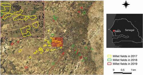
The study area is located in the mid-western part of Senegal (Fatick Province) near the Diohine village (Figure 1). The site covers around 17 km² of the groundnut basin, which is one of the main agroecological zones in the country. The Senegalese groundnut basin is essentially flat and dominated by rainfed agriculture and smallholder farming. The study area is characterized by a tree-based cropping system, dominated by Faidherbia albida, a nitrogen-fixing species with unique reverse phenology that is known to have a boosting effect on the yields of the crops with which it is associated (Sileshi 2016). The cropland includes mainly millet and groundnut. The former is grown for consumption while the latter is a cash crop. Other crops such as sorghum or cowpea are cultivated solely or intercropped with millet. The climate is of the Sudano-Sahelian type, characterized by a rainy season from July to October and a long dry season that extends over the rest of the year. Average annual rainfall varies between 400 mm and 650 mm.

Figure 1. Location of the study area and the sample fields included in the work for which yield measurements were conducted. Note that five fields were monitored in both 2018 and 2019. The zoom at the top left highlights the presence of trees in the fields. Bing Maps images are displayed in the background

2.1.2. Field data

The study was conducted over three agricultural seasons (2017, 2018, and 2019) and focused on pearl millet cultivation, a staple crop in the region. Millet fields are usually sowed in dry conditions between late May and early July and harvested between September and October. The millet grown by farmers in the region is Souna a short-cycle variety (90 days), characterized by a vegetative growth stage that lasts approximately until mid-August or early September, followed by the reproductive growth stage where grain filling occurs. A total of 66 fields were monitored: 35 in 2017, 15 in 2018, and 16 in 2019 (see Figure 1). 81% of monitored plots have a mixed cropping system (basically millet intercropped with sorghum or cowpea), and the average plot size is about 0.63 ha. Within each field, three representative millet quadrants of 6 m² were randomly selected. Above-ground biomass was harvested in each quadrant at crop maturity and grain yield (dry matter) was measured after drying at 70°C for 48 h. In addition, some information about agricultural practices was recorded (e.g. sowing and harvest dates, observed dates of different phenological stages: emergence, maturity, senescence). Figure 2 shows the per-year distribution of the millet yields over sample fields and evidences the year-to-year variability as well as the high spatial heterogeneity within a year (e.g. 2017 and 2019). The main driving factors causing the yield variability between years are related to the onset of the rainy season that determines the agricultural calendar and thus influences final crop yields (Marteau et al. 2011). Since agriculture is rainfed, a long interruption of rainfall after sowing can lead to reseeding of plots and hence impact the final yields. In addition to the rainfall factor, the crop rotation practice on plots, the amount of nutrients applied from year to year, together with the poor soil fertility, are also determinants of final yields, as recently evidenced over our study area by (Leroux et al. 2020). Observed yields range from 239 kg/ha to 3278 kg/ha, with average and median yields of 1184.51 kg/ha and 976.5 kg/ha, respectively.

Figure 2. Per year distribution of the millet yields over sample fields showing a high year-to-year variability. Overall, recorded yield values in 2018 are lower than in 2017 and 2019 and most of these values are distributed around 900 kg/ha, contrary to other years where the values are more uniformly distributed

2.1.3. Satellite data

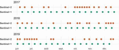
We considered in this study modern Earth Observation satellites, namely Sentinel-1 and Sentinel-2, to analyse the contribution of multi-source (SAR and optical) data for the millet yield assessment. Results from Leroux et al. (2014) over the Sahelian zone suggested that a spatial resolution of 10-m may be sufficient for crop monitoring in such heterogeneous agricultural landscape characterized by small to very small fields (Fritz et al. 2015). The image time series were collected throughout each growing year from early June to the end of December, with a total of 17 images per source and per year (Figure 3). We included images covering several weeks before sowing and several weeks after harvest in order to cover as much as possible the information related to a complete growing cycle of the fields (full ascending and descending).

Figure 3. Overview of the acquisition dates of Sentinel-1 (S1) and Sentinel-2 (S2) images over three agricultural seasons. S2 acquisitions are sparsed due to the ubiquitous cloudiness

The Sentinel-1 (SAR) images were retrieved from the PEPS processing platform (peps.cnes.fr) at level-1 C Ground Range Detected (GRD). The Sentinel-1 images were acquired in C-band, Interferometric Wide Swath (IW) mode with dual polarization (VH and VV) and ascending orbit. First, we radiometrically calibrated the images in backscatter coefficient values (decibels, dB) using parameters included in the metadata and then orthorectified them at the spatial resolution of 10-m. Finally, multi-temporal filtering (Quegan and Yu 2001) was applied to the images in order to reduce the speckle effect. The filtering produces speckle-reduced images from inputs by linearly combining multi-looked backscatter intensity/coefficient values, sampled at different timestamps, with a local mean estimated by averaging values in a local window around each pixel in each image.

The Sentinel-2 (optical) images were retrieved from the THEIA processing platform (theia.cnes.fr) at level-2A, in top-of-canopy (TOC) reflectance values with cloud masks. We only kept cloudless images over the sample fields. Ten spectral bands were then retained: the 10 m spatial resolution bands (Blue, Green, Red, Near Infrared) and those at 20 m spatial resolution (4 Red edge and 2 Short-wave Infrared). The 20 m bands were all resampled at 10 m spatial resolution using the nearest neighbour method. A preprocessing was performed over each band to replace remaining cloudy pixel values as detected by the supplied cloud masks through a linear multi-temporal interpolation (cf. temporal gap-filling (Inglada et al. 2017)). Seven vegetation indices (VI) were subsequently derived from the optical bands as proxies for the vegetation activity (Table 1).

Table 1. Vegetation indices derived from optical bands (Band abbreviations: B–Blue, G–Green, R–Red, RE–Red edge, NIR–Near Infrared, SWIR–Short Wavelength Infrared)

Vegetation index	Name and reference	Formula
NDVI	Normalized Difference Vegetation Index (Rouse et al. 1973; Tucker 1979)	$\frac{NIR-R}{NIR+R}$
NDWI	Normalized Difference Water index (Cai Gao 1996)	$\frac{NIR-SWIR}{NIR+SWIR}$
MSAVI2	Modified Soil Ajusted Vegetation Index (Qi et al. 1994)	$\frac{2\times NIR+1-\sqrt{{(2\times NIR+1)}^2-8\times (NIR-R)}}{2}$
EVI	Enhanced Vegetation index (Jiang et al. 2008)	$2.5\times \frac{NIR-R}{NIR+6R-7.5B+1}$
GDVI	Green Difference Vegetation Index (Tucker 1979)	$NIR-G$
CIgreen	Chlorophyll Index green (Gitelson, Gritz, and Merzlyak 2003)	$(\frac{NIR}{G}{)}^{-1}$
CIrededge	Chlorophyll Index red edge (Gitelson, Gritz, and Merzlyak 2003)	$(\frac{NIR}{RE}{)}^{-1}$

The SAR backscatter in dual-polarization, optical bands, and VI time series (see Appendix A for a summary of variables used) was normalized per year in the interval [0,1]. Then, median values were extracted from the multi-source and multi-year data at the field scale. Median statistics fit well smallholder farming context since they are not sensitive to extreme values, which can occur due to intra-plot variability induced by different management strategies, the presence of trees, or termite nests (Félix et al. 2018). Therefore, we did not consider tree masking in this study and also since preliminary experiments showed no significant influence on our modelling approaches. With the aim of forecasting the millet yields, we linearly interpolated the multi-source and the multi-year time series on a regular grid as the acquisition dates are variable per source and per year. Interpolation and resampling were performed on a 5 day basis over the data acquisition period.

2.1.4. Millet patches

In order to map the millet yields at field scale over the study site, we generated millet patches (Figure 4). We defined millet patches as pseudo plots of millet with similar biophysical and management characteristics. To this end, we first performed a superpixel segmentation of the study site using the SLIC algorithm (Li and Chen 2015) on a high spatial resolution PlanetScope NDVI time series acquired over the 2018 growing season. Subsequently, for each growing year excepted 2017, candidate patches (segments) were spatially intersected with an object-based Land Use/Land Cover (LULC) map of the study area. Finally, millet patches were obtained by a majority vote of the LULC class extracted for intersected patches and by excluding the non-cereal segments. The millet patches and subsequently the yield mapping were not carried out in 2017 due to budgetary limitations that prevented the collection of ground truth samples and thereby the production of the LULC map for this specific year. Note that the generation of millet patches is independent of the task of yield modelling where field samples were monitored for the 3 years included in the study. The LULC map is obtained via our previous work (Gbodjo et al. 2020). For this purpose, independently from the 66 millet plots, we monitored in this study, we built ground truth samples from GPS land cover records that were collected in 2018 and 2019. A total of 3084 samples (respectively, 2892 samples) distributed over nine classes (see Table 2) were used to produce the 2018 (respectively, 2019) LULC map. Both 2018 and 2019 LULC maps were classified with reasonable overall accuracy (resp., 90% and 79%) and cereal class F1-score (resp., 88% and 77%).

Figure 4. Candidate and final patches for the spatialization of millet yields over 2018 and 2019 growing seasons. Bing Maps images are displayed in the background of subfigures 4e and 4f. The maps were created with https://www.qgis.org/fr/site/forusers/download.htmlQGIS 3.14

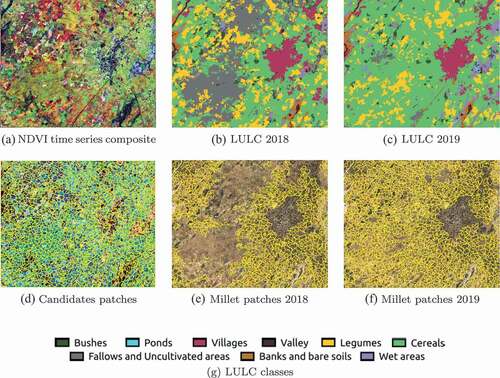
Table 2. Characteristics of the ground truth data used for LULC mapping

Class	Label	2018 Samples	2019 Samples
1	Bushes	100	100
2	Fallows and Uncultivated areas	322	57
3	Ponds	59	59
4	Banks and bare soils	132	132
5	Villages	767	767
6	Wet areas	156	156
7	Valley	56	56
8	Cereals	816	1038
9	Legumes	676	527
Total		3084	2892

2.2. Methods

2.2.1. Modelling approaches

Linear regression (LR) This is our baseline. We performed a simple linear regression model with a unique predictor the maximum of NDVI value recorded during the growing cycle. The potential of this baseline has already been highlighted in different agricultural contexts (Azzari, Jain, and Lobell 2017; Jain et al. 2016; Lambert et al. 2018). Since a majority of cereal crop yields are determined by the photosynthetic activity for the period from flowering to harvest (Rembold et al. 2013), the NDVI value at the peak of the season is considered as a valuable predictor of the final yields.

Ridge regression (RR) (Hoerl and Kennard 1970) This is a multiple regression method that uses $L^2$ (euclidean) norm regularization as a penalty term. RR helps prevent multi-collinearity by shrinking the predictor coefficients and reduces the model complexity. A penalty parameter is used to control the strength of the regularization.

Random Forest (RF) (Breiman 2001) is an ensemble learning method that uses multiple decision trees to improve accuracy and prevent overfitting. The trees are grown independently on slightly different subsets of training data using a bootstrap technique (i.e. random sampling with replacement) and then aggregated in a bagging process by averaging predictions in case of a regression problem. RF is known to be robust to multi-collinearity in data due to its bootstrap aggregation procedure.

Multi-Layer Perceptron (MLP) (Rumelhart, Hinton, and Williams 1986) Sometimes also called Artificial neural networks or deep feedforward networks (Goodfellow, Bengio, and Courville 2016), the MLP is a type of feedforward neural network that consists of an input layer, some number of non-linear or hidden layers and an output layer, which are fully connected. It learns to approximate a function that best maps inputs to desired outputs. Learning is done using the backpropagation algorithm (Rumelhart, Hinton, and Williams 1986).

Long Short-Term Memory (LSTM) (Hochreiter and Schmidhuber 1996) This is an advanced variant of Recurrent Neural Network (RNN) that deals with the vanishing and exploding gradient issues of vanilla RNN. Unlike feedforward networks, RNNs are designed to process sequential data and thus are well suited for time series since the output at a time step is used to feed the model at the next time step of the sequential processing. LSTM explicitly accumulates information in a cell state and controls its flow by various gates.

Convolutional Neural Network (CNN) (LeCun et al. 1989) It is a family of feedforward neural networks that process data of a known grid such as images (2D grid) or time series with regular sampling (1D grid) as in our case. CNN, as his name implies, operates by convolution kernels (Dumoulin and Visin 2016). Convolutions are followed in CNN architectures by non-linear activation functions, pooling layers that aggregate or filter values using operators like average or maximum, and subsequently fully connected layers. CNN explicitly learns feature representations and captures patterns in data that are relevant for the particular task at hand.

Six approaches in total were then benchmarked for the task of millet yield modelling. The LR, RR, and RF models were implemented using the Python Scikit-learn library (Pedregosa et al. 2011). We optimized the RR and RF models by varying the penalty parameter for the former and the number of trees as well as the number of features and the depth of the decision trees for the latter. The range of values associated with these hyperparameters is reported in Table 3. To implement the neural network models, we used the Python Tensorflow library. Given the small size of our dataset, we designed the MLP, LSTM, and CNN benchmarks with lightweight architectures. The MLP is thus set up with two hidden layers with 64 units, each followed by the Rectified Linear Unit (ReLU) non-linearity activation. Similarly, the LSTM model is set up with 64 hidden units. To design the CNN, we followed some general guidelines adopted in the literature where the number of filters grows along with the network. Our CNN architecture consists of six convolutional layers with a maximum of 64 filters followed by a Pooling layer. The rest of its architectural details is reported in Table 4. We employed the Huber loss as a cost function for the neural networks, and the Adam optimizer (Kingma and Ba 2014) was used to learn the parameters of the models. Since the learning of these parameters can be critical owing to the size of the dataset, we adopted the moving average technique to obtain the final model weights. The learning rate, batch size, and the number of epochs associated with the learning stage are reported in Table 3.

Table 3. Hyperparameter settings of the different approaches considered for millet yield estimation. RR and RF hyperparameters were optimized by varying associated values while MLP, LSTM, and CNN hyperparameters were empirically fixed

Method	Hyperparameters	Value or range
RR	Penalty term	{0.001,0.1,1}
RF	Number of trees	{50, 100, 200}
	Maximum depth	{10, 20, 50, None}
	Maximum features	{’sqrt’, ’log2ʹ, None}
MLP	Learning rate	1e-3
LSTM	Batch size	1
CNN	Number of Epochs	1000

Table 4. Details of the CNN architecture: Conv stands for Convolution operation, $nf$ is the number of filters, $k$ is the kernel size, $s$ is the stride value, and $act$ is the activation function. As for precedent neural network models, we used a maximum number of filters of 64

Block 1	Conv($nf$=16, $k$=5x1, $s$=1, $act$=ReLU)
Block 2	Conv($nf$=16, $k$=3x1, $s$=1, $act$=ReLU)
Block 3	Conv($nf$=32, $k$=3x1, $s$=2, $act$=ReLU)
Block 4	Conv($nf$=32, $k$=3x1, $s$=1, $act$=ReLU)
Block 5	Conv($nf$=64, $k$=1x1, $s$=1, $act$=ReLU)
Block 6	Conv($nf$=64, $k$=1x1, $s$=1, $act$=ReLU)
Block 7	Global MaxPooling()

2.2.2. Estimating, forecasting, and mapping the millet yields

The estimating approach was based on the non-interpolated time series (17 acquisitions per source and per year) collected throughout the crop growing cycle. Millet yields were first estimated using each set of predictors (i.e. SAR, optical, and VI) separately. Then, we assessed the benefit to combine multi-source data to estimate millet yields. This leads to four combination scenarios in which input sources are concatenated: (i) SAR backscatter in dual-polarization and optical bands, (ii) SAR and VI, (iii) optical bands and VI, and (iv) all feature set, i.e. SAR, optical bands, and VI. Finally, the best scenario considering the model performances and the features used was further explored in the forecasting approach.

The forecasting approach was based on the interpolated time series with a 5 day interval and was carried out over a time period that spans from the start of the acquisitions in early June to late October at the end of the season. Various time windows of the interpolated time series were considered in order to figure out a suitable period before harvest where accurate and satisfactory yields forecast could be obtained. Millet yields were predicted from the emergence (early July) to the senescence stage considering time windows shortened by 15-day increments from the beginning. The 15-day interval was found as a reasonable period of time, allowing significant changes for vegetation.

Lastly, yield mapping was carried out on 2018 and 2019 millet patches, also considering the best models resulting from both approach experiments (i.e. estimation and forecasting).

2.2.3. Evaluation of modelling approaches

We assessed the performance of the models using a 3-fold cross-validation procedure randomly repeated 10 times. One-quarter of the training fold (about 11 out of 44 sample fields) was used to validate models, i.e. to select the best hyperparameters for RR and RF or to save the best weight configuration at the training epochs for neural networks. Predictions were made using the test fold (about 22 sample fields), and finally, model performances were averaged and reported considering the following metrics: the coefficient of determination (R²), the Mean Absolute Error (MAE), and the Root Mean Squared Error (RMSE). The metric formulas are displayed below:

$R^2=1-\frac{{\sum }_{j=1}^n{(y_j-{\hat{y}}_j)}^2}{{\sum }_{j=1}^n{(y_j-\bar{y})}^2}MAE=\frac{1}{n}\sum _{j=1}^n|y_j-{\hat{y}}_j|RMSE=\sqrt{\frac{1}{n}\sum _{j=1}^n{(y_j-{\hat{y}}_j)}^2}$

where $n$ is the total number of observations; $y_j$ is the $j^{th}$ observed sample value; ${\hat{y}}_j$ is the $j^{th}$ predicted sample value, and $\bar{y}$ is the mean of observed values.

3. Results

3.1. Estimation of millet yields

3.1.1. Estimation with mono-source predictor variables

The average performances of the models are reported in Table 5. First, we note that the baseline approach (LR with maximum observed NDVI values) does not perform well with a low average $R^2$ score of 0.08. As concerns other approaches, they perform better than the baseline. Regardless of the predicting features, RF and MLP models achieved comparable scores (average $R^2$ of 0.48) and performed better than all other approaches, i.e. DL models (LSTM and CNN), which obtained similar scores (average $R^2$ of 0.42) and RR (average $R^2$ of 0.41). Considering input sources, we first note that SAR information is less effective than optical one (spectral bands or vegetation indices (VI)) for our millet yield modelling task, as can be observed especially for CNN (average $R^2$ of 0.06). In addition, the models behave differently with respect to optical bands and VI variables since RR and MLP achieved better results with optical bands while, conversely, RF, LSTM, and CNN performed better with VI. Overall, RF model trained on VI predictors and MLP model fed with optical data were the best scenarios to estimate millet yields from the mono-source data, obtaining similar results (e.g. an average RMSE of 446 kg/ha and 445 kg/ha, respectively). Figure 5 depicts the observed versus predicted millet yields (average over the cross validation procedure) scatter plots considering the modelling approaches. Following average behaviour, the CNN model that deals with VI time series exhibits better agreements than other approaches, although marginal box plot distributions reveal overestimation (resp. underestimation) of low (resp. high) observed yields from all approaches. To wrap up, common regression methods in crop yield modelling such as RF and MLP outperformed the considered DL approaches (i.e. LSTM and CNN) in our study area regarding the evaluation metrics for the millet yield estimation.

Figure 5. Scatter plots of the observed versus predicted millet yields averaged over the 10 repeated 3-fold cross validation procedure considering Ridge Regression (RR), Random Forest (RF), Multi-Layer Perceptron (MLP), Long Short-Term Memory (LSTM), and Convolutional Neural Network (CNN) models and the set of predictor variables (i.e. SAR, optical, and VI)

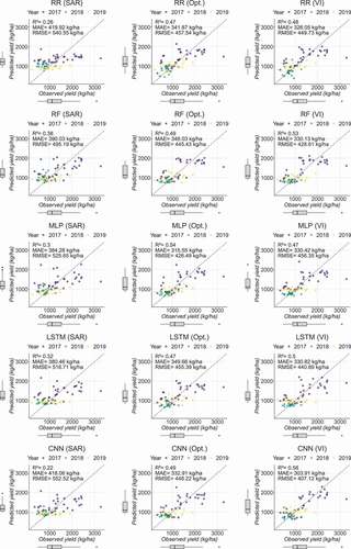
Table 5. Average performances of the Linear Regression (LR), Ridge Regression (RR), Random Forest (RF), Multi-Layer Perceptron (MLP), Long Short-Term Memory (LSTM) and Convolutional Neural Network (CNN) models over the 10 repeated 3-fold cross validation procedure. The baseline (LR model) was performed using the maximum observed NDVI value over the growing cycle as unique predictor

Max. NDVI	$R^2$	MAE	RMSE
LR	0.08$\pm$0.13	473.27$\pm$44.32	593.66 $\pm$ 63.31
SAR	$R^2$	MAE	RMSE
RR	0.24$\pm$0.14	422.28$\pm$34.94	539.98 $\pm$ 64.08
RF	0.32$\pm$0.15	400.39$\pm$43.70	509.53 $\pm$ 71.23
MLP	0.20$\pm$0.26	409.49$\pm$54.39	547.38 $\pm$ 100.18
LSTM	0.25$\pm$0.19	397.37$\pm$46.47	533.81 $\pm$ 85.29
CNN	0.06$\pm$0.23	451.25$\pm$55.23	597.27 $\pm$ 86.67
Optical	$R^2$	MAE	RMSE
RR	0.41$\pm$0.20	360.65$\pm$55.26	471.03 $\pm$ 90.99
RF	0.44$\pm$0.12	361.5$\pm$37.14	460.83 $\pm$ 68.65
MLP	0.48$\pm$0.17	335.5$\pm$52.24	445.0$\pm$ 87.85
LSTM	0.33$\pm$0.19	391.58$\pm$51.42	500.68 $\pm$ 71.15
CNN	0.35$\pm$0.17	377.28$\pm$60.70	497.10 $\pm$ 84.35
VI	$R^2$	MAE	RMSE
RR	0.36$\pm$0.17	381.29$\pm$55.52	492.39 $\pm$ 86.52
RF	0.48$\pm$0.13	346.06$\pm$41.0	446.32 $\pm$ 67.77
MLP	0.42$\pm$0.14	348.41$\pm$40.68	471.15 $\pm$ 73.12
LSTM	0.42$\pm$0.12	358.60$\pm$48.88	468.92 $\pm$ 68.97
CNN	0.42$\pm$0.21	360.11$\pm$67.56	468.91 $\pm$ 94.68

3.1.2. Estimation with combination scenarios of predictor variables

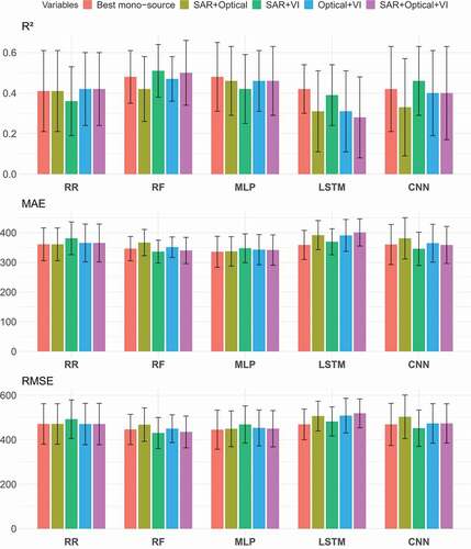
In Figure 6, we illustrate the average performances of the models considering four combination scenarios of the multi-source data: SAR and optical bands, SAR and VI, optical bands and VI and finally SAR, optical bands, and VI. For comparison purpose, we also reported the best performances obtained with mono-source data. Except RF and CNN models, we note lower or similar performances to those previously obtained by the models. Considering $R^2$ metric, RF improves from 0.48 to 0.51, while CNN improves from 0.42 to 0.46. Both models obtained their best scores with SAR and VI combination scenario which is also more effective than other scenarios in the case of LSTM. However, such combination scenario performs worst for RR and MLP models. Overall, the multi-source (SAR and optical) combination did not systematically improve the millet yield estimation. Also, observed improvements seem to be tightly linked with the modelling approach.

Figure 6. Average performances (standard deviation as error bar) of Ridge Regression (RR), Random Forest (RF), Multi-Layer Perceptron (MLP), Long Short-Term Memory (LSTM), and Convolutional Neural Network (CNN) models over the 10 repeated 3-fold cross validation procedure considering the four combination scenarios of predictor variables (i.e. SAR+Optical, SAR+VI, Optical+VI, SAR+Optical+VI). We referred to as ‘Best mono-source’ the best performances obtained from individual feature set (within optical and VI time series)

3.2. Forecasting of millet yields

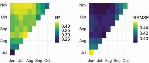
In order to deal with the millet yield forecasting, we employed the RF model with SAR and VI combination as input, since it gave the best performances regarding the estimation approach (see Figure 6). Figure 7 illustrates the yield forecast results from the emergence to senescence stage considering various time windows shortened by 15-day increments. We note that the forecast accuracy increases significantly, as considered time windows get close to the harvest period in late October. The RF model achieved acceptable results for a prediction period that ranges from mid-August to late October. Even the best results, considering the evaluation metrics, were obtained for the time period that spans from mid-July to mid-August ($R^2=0.44$), stable predictions are clearly achieved from mid-October ($R^2=0.43$), around 2 weeks before the end of the cropping season. In addition, the forecast accuracy is, overall, not highly sensitive to the length of time windows, since similar performances can be achieved for a specific prediction period. Note, however, that late time windows (within early September and late October) probably achieved lower results since predictions are mainly based on senescence stage information.

Figure 7. Average performances (considering $R^2$ and Relative RMSE metrics) of the Random Forest (RF) model with SAR and VI combination as input for forecasting millet yields from the emergence to senescence stage via time windows shortened by 15-day increments from the beginning. The x (resp. y) axis represents the beginning (resp. the end) of the time window

3.3. Mapping of millet yields

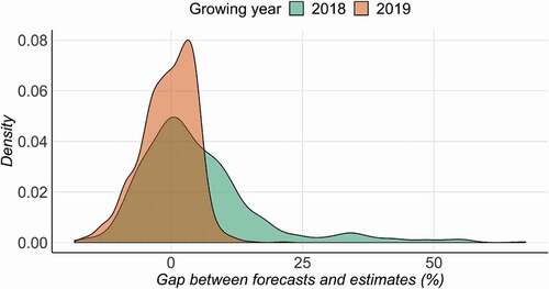
Lastly, Figure 8 illustrates the millet yield mapping for 2018 and 2019 millet patches, considering the RF model with SAR and VI predictors as input. In addition, we have computed the gap between yield forecasts and yield estimates with the aim to evaluate misestimations of the yield forecasting around 2 weeks before the end of the season, i.e. in mid October. This analysis was not carried out in 2017 due to budgetary limitations that prevented the production of land cover map for this specific year (see Millet patches section). First, we observe that yield maps (Figures 8(a,c)) exhibit notable spatial variability in both years, even for contiguous patches. Average yield estimates for millet patches were of 965 kg/ha with a coefficient of variation of 8% in 2018 (respectively 1080 kg/ha with a coefficient of variation of 17% in 2019). Not surprisingly, comparatively high yields were obtained in the fertility ring, i.e. patches surrounding living areas (villages) while remote patches exhibit much more lower yields. An example is given by the former fallow areas (the entire western part of the 2018 map), grown in 2019, which exhibit low yields. As regards the gaps between forecasts and yield estimates (Figures 8(b,d)), the RF model clearly overestimates final yields in 2018, especially in the fertility ring, while, in 2019, final yields are overall underestimated for this particular area. Average gaps were about 5% in 2018 and −0.5% in 2019. Accordingly, there is no clear tendency from one year to the next with respect to the gaps exhibited by a same area. However, most of the prediction errors for the millet patches remain low, indicating satisfactory forecasting capabilities, as evidenced by their distributions in Figure 9.

Figure 8. Millet yield mapping and gap between forecasts and estimates for 2018 and 2019 agricultural seasons using the Random Forest (RF) model and SAR as well as VI combination as input. Yield forecasting was achieved at mid October. A quantile discretization was applied to the maps. Bing Maps images are displayed in background. The maps were created with https://www.qgis.org/fr/site/forusers/download.htmlQGIS 3.14

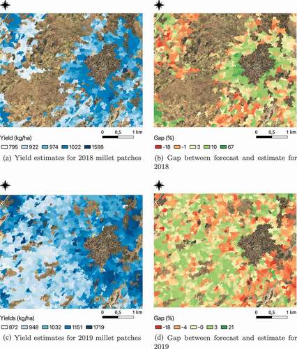
Figure 9. Distribution of gaps between yield forecasts and yield estimates for 2018 and 2019 millet patches. Most of the prediction errors are low

4. Discussion

In this work, we proposed to perform as baseline approach for the millet yield estimation, a simple LR model using the highest NDVI value observed over the growing cycle as unique predictor. The baseline failed to explain the millet yield variability in the study site ($R^2$=0.08). The potential of this approach has already been highlighted in various studies (Azzari, Jain, and Lobell 2017; Jain et al. 2016; Lambert et al. 2018). However, in this work, the peak activity period (around early/mid-September) is poorly covered by optical images due to the ubiquitous cloudiness. Therefore, the maximum NDVI value observed over the growing season is probably underestimated and such a factor could have seriously impacted the quality of the linear regression.

Among other approaches, DL models i.e. LSTM and CNN have performed lower than common regression methods in crop yield modelling, namely RF and MLP. Considering recent trends in literature (Wolanin et al. 2020; You et al. 2017), these results are unexpected but we should note that our study context is quite challenging for DL approaches. Such methods have mainly exhibited their effectiveness, with respect to common machine learning techniques, in scenarios where they learn from large scale data. Therefore, we consider that the small size dataset we dispose in this study (66 samples fields) is not sufficient to allow DL models to learn useful and generalizable representations associated to the task of yield modelling. This is probably the reason why the best performances of the DL models (CNN and LSTM) were achieved with the VI as input ($R^2$=0.42) instead of the raw data (SAR backscatter or optical bands). The VI input can be seen as handcrafted features since they are derived from a combination of raw data. Nonetheless, it is noteworthy that the CNN, in particular, has exhibited potential even in this challenging scenario. Average performances are overall not so far from RF and MLP ($R^2$=0.48) and Figure 5 has especially highlighted better agreements in favour of CNN, as regards the scatter plots of the observed versus predicted yields.

Another key aspect investigated in this work was linked to the assessment of millet yield using multi-source remote sensing data i.e. SAR and optical. We first employed each source separately and achieved better results considering optical/VI instead of SAR predictors. Despite the successful use of SAR data in various crop monitoring studies (Fieuzal and Baup 2017), such result is not surprising, since biophysical processes information supplied by optical data are probably more meaningful here than the SAR backscatter, which mainly contains information on the structure (leaves and canopy), moisture content of the vegetation and the underlying soil. Subsequently, we combined the multi-source data by investigating four possible scenarios. Among tested configurations, only SAR and VI combination overall improves our results but, as observed, such improvements were tightly linked to the modelling approach. Since SAR and optical signals are known to be complementary (Ienco et al. 2019; Jin et al. 2019), it is surprising that only RF and CNN were able to effectively exploit them to improve the millet yield modelling, while other models (RR, MLP, and LSTM) were not. However, such result with MLP exists in the literature. Fieuzal, Marais-Sicre, and Baup (2017) used microwave data (TerraSAR-X and Radarsat-2) and optical data (Formosat-2 and Spot-4/5) to model corn yield on about 30 sample fields in southwestern France. Among various configurations including interactions between the multi-source data (SAR backscatter in various polarizations and optical wavelengths), the best estimation was obtained in the red wavelength while no gain in performances was achieved by combining the multi-source information. Following similar setting, Fieuzal and Baup (2017) forecasts wheat yield from SAR and optical data and, as in this case, the best in-season yield forecast was not achieved using a multi-source (i.e. radar and optical) combination. It is conceivable that in the challenging context of limited samples which defines most of crop yield monitoring studies, particularly in smallholder farming systems, not all modelling approaches are suitable to leverage multi-source dependencies like in crop type/land cover mapping scenarios (Denize et al. 2019; Gbodjo et al. 2020) where more data is available.

In this work, we have also conducted the forecasting of millet yields throughout the cropping season in order to figure out a suitable period before harvest where satisfactory forecasts of millet yields could be obtained on the study area. Given the explanatory power of the RF model, stable and satisfying forecasts were obtained in mid-October i.e. 2 weeks before the end of season. Early estimates in the growing season can considerably improve the efficiency of political responses to food shortage issues and it is noteworthy that in Senegal, official crop yield statistics are available few months after the harvest period, typically at the end of November. These statistics are obtained traditionally from field campaigns using stratified sample strategies which are time consuming and costly (Jacques and Defourny 2019). As observed here, remote sensing-based regression modelling methods remain useful tools that can help speed up the collection of crop production information in the study area and then improve the response time to emergency situations. However, rather than replace traditional ground-based collection efforts, we argue that these approaches should complement them. Successively, we conducted the millet yield mapping over the study area, at field scale, using 2018 and 2019 millet patches. Besides the pure crop acreage and crop yield estimate applications, mapping crop yields in SSA smallholder farms can further help analyse spatial heterogeneity and give insights on appropriate strategies aiming to guide agronomic practices and minimize such disparities. For instance, Jin et al. (2019) and Leroux et al. (2020) investigated for maize and millet crops, respectively, the drivers of yield spatial variability among management practices and biophysical factors like soil nutrients. Here, the high yield values obtained for millet patches close to living areas with respect to remote patches, suggest that livestock manure intakes are a determinant of the spatial heterogeneity in the study area, since they are mainly spread out around households. In addition, we analysed the gap between forecasts and estimates for 2018 and 2019 millet patches. Forecasts were mainly overestimated in 2018 and underestimated in 2019. Overall, we did not found any clear spatial tendency between the years regarding the gaps exhibited for a particular area. Several factors linked to the inter-annual variability existing in SSA smallholder agriculture may be worth considering to explain these dissimilarities. For instance, environmental effects (e.g. onset of the rainy season) or agricultural practices (e.g. crop rotation, inter-cropping, amount of organic or chemical input applied) are all elements which cause heterogeneity of cropping seasons between years. Therefore, it can be problematic to obtain similar trends between years by considering the same time windows for predictor variables in the forecasting approach. Lastly, we would like to remind that the whole analysis which results from the millet yield mapping is intrinsically linked to the quality of input land cover mapping, thus classification confusion errors can introduce possible biases in the subsequent reasoning.

We also emphasize that our study was conducted on a small scale area of around 17 km², owing mainly to the paucity of observed data and we highlight that the availability of ground truth data, especially for staple crops like millet, is the major factor that still prevents the scalability of numerous smallholder crop yield monitoring research studies in SSA countries.

5. Conclusion

A sustainable growth in SSA countries can be achieved through proper policies and investments aiming at improving smallholder agriculture productivity. In order to inform and assist decision-makers, timely and accurate monitoring of smallholder farming systems is critical. While remote sensing remains a major asset for crop yield monitoring at a fine scale, few studies have leveraged multi-source (SAR and optical) satellite images in the context of small-scale agriculture in SSA. In addition, promising modelling approaches such as DL techniques have only received little attention for crop yield monitoring in SSA countries. This study tackles the estimation and forecasting of pearl millet yields using multi-source (SAR and optical) remote sensing data and regression modelling approaches in the Senegalese groundnut basin. A large panel of modelling approaches was employed, ranging from the usual regression models in crop yield modelling to DL techniques designed to deal with multivariate time series. Among the tested approaches, an RF model explains up to 50% of the millet yield variability in the study area, while CNN shows promise results but performs lower. The combination of multi-source data, particularly SAR polarizations and vegetation indices, improved the crop yield modelling task, but such improvement was tightly linked to the modelling approach, namely RF and CNN. Using the RF model, we forecast the millet yields and reached stable and satisfactory accuracy 2 weeks before the end of the season. Our results reinforce the use of RF, a well known and established approach to assess crop yields, notably in the context of small scale agriculture and, last but not least, show the potential of DL approaches, especially CNN, which could become a standard also for crop yield monitoring in SSA countries with strategies like self or semi-supervised learning (Jing and Tian 2020; Yang et al. 2021) instead of end-to-end supervised learning that requires more ground reference data. As an alternative to collecting more reference data in order to enhance the capabilities of DL or empirical modelling approaches in general, one strategy can be to focus on determining further relevant explanatory variables. One way could be to densify the optical time series using acquisitions from multi-platforms (e.g. Sentinel-2, PlanetScope, or Véns). This approach is expected to fill common gaps at critical phenological stages of the cropping season that influence final yields. Another direction could be complementing pure remote sensing-based predictors with a set of bioclimatic/soil-related variables as well as yield correlated outputs generated from crop simulation models, which have been found to improve empirical methods (Azzari, Jain, and Lobell 2017; Leroux et al. 2019). Finally, another possible future work can be devoted to investigate the synergistic use of UAVs and satellite data as a potential way to improve crop yield prediction in SSA smallholder agriculture.

Acknowledgements

The authors are very thankful to PhD students (Sophie Djiba, Adama Tounkara, and Medoune Mbengue) for sharing their agronomic data for the 2017 cropping season.

Disclosure statement

No potential conflict of interest was reported by the author(s).

Additional information

Funding

This work was supported by the French National Research Agency under the Investments for the Future Program, referred as ANR-16-CONV-0004 (DigitAg), the LYSA project (DAR-TOSCA 4800001089) funded by the French Space Agency (CNES), the SERENA project funded by the Cirad-INRA metaprogramme GloFoodS, the SIMCo project (agreement number 201403286-10) funded by the Feed The Future Sustainable Innovation Lab (SIIL) through the USAID AID-OOA-L-14-00006 and the CGIAR Research Program on Grain Legumes and Dryland Cereals (GLDC);Agence Nationale de la Recherche;

Appendix A

Summary of variables used for millet yield prediction

Table

Type of variables	List of variables
SAR (Sentinel-1)	Backscatter coefficient in C band with co and cross polarization VV and VH
Optical bands (Sentinel-2)	B2,B3,B4,B8,B5,B6,B7,B8A,B11,B12
Optical vegetation indices (Sentinel-2)	NDVI, NDWI, MSAVI, EVI, GDVI, CIgreen et CIrededge

References

- Azzari, G., M. Jain, and D. B. Lobell. 2017. “Towards Fine Resolution Global Maps of Crop Yields: Testing Multiple Methods and Satellites in Three Countries.” Remote Sensing of Environment 202: 129–141. In press. doi:https://doi.org/10.1016/j.rse.2017.04.014.
- Becker-Reshef, I., B. Barker, M. Humber, E. Puricelli, A. Sanchez, R. Sahajpal, K. McGaughey, et al. 2019. “The GEOGLAM Crop Monitor for AMIS: Assessing Crop Conditions in the Context of Global Markets.” Global Food Security 23: 173–181. doi:https://doi.org/10.1016/j.gfs.2019.04.010.
- Breiman, L. 2001. “Random Forests.” Machine Learning 45 (1): 5–32. doi:https://doi.org/10.1023/A:1010933404324.
- Burke, M., and D. B. Lobell. 2017. “Satellite-based Assessment of Yield Variation and Its Determinants in Smallholder African Systems.” Proceedings of the National Academy of Sciences 114 ( 9): 2189–2194.
- Cai Gao, B. 1996. “NDWI—A Normalized Difference Water Index for Remote Sensing of Vegetation Liquid Water from Space.” Remote Sensing of Environment 58 (3): 257–266. doi:https://doi.org/10.1016/S0034-4257(96)00067-3.
- Davis, B., S. Di Giussepe, and A. Zezza. 2017. “Are African Households (Not) Leaving Agriculture? Patterns of Households’ Income Sources in Rural Sub-Saharan Africa.” Food Policy 67: 153–174. doi:https://doi.org/10.1016/j.foodpol.2016.09.018.
- Denize, J., L. Hubert-Moy, J. Betbeder, S. Corgne, J. Baudry, and E. Pottier. 2019. “Evaluation of Using Sentinel-1 and −2 Time-Series to Identify Winter Land Use in Agricultural Landscapes.” Remote Sensing 11 (1): 37. doi:https://doi.org/10.3390/rs11010037.
- Dumoulin, V., and F. Visin. 2016. “A Guide to Convolution Arithmetic for Deep Learning.”
- Félix, G. F., I. Diedhiou, M. Le Garff, C. Timmermann, C. Clermont-Dauphin, L. Cournac, J. C. J. Groot, and P. Tittonell. 2018. “Use and Management of Biodiversity by Smallholder Farmers in Semi-arid West Africa.” Global Food Security 18: 76-85.
- Fieuzal, R., and F. Baup. 2017. “Forecast of Wheat Yield Throughout the Agricultural Season Using Optical and Radar Satellite Images.” International Journal of Applied Earth Observation and Geoinformation 59: 147–156. doi:https://doi.org/10.1016/j.jag.2017.03.011.
- Fieuzal, R., C. Marais-Sicre, and F. Baup. 2017. “Estimation of Corn Yield Using Multi-temporal Optical and Radar Satellite Data and Artificial Neural Networks.” International Journal of Applied Earth Observation and Geoinformation 57: 14–23. doi:https://doi.org/10.1016/j.jag.2016.12.011.
- Foley, J. A., N. Ramankutty, K. A. Brauman, E. S. Cassidy, J. S. Gerber, M. Johnston, N. D. Mueller, et al. 2011. “Solutions for a Cultivated Planet.” Nature 478 (7369): 337–342. doi:https://doi.org/10.1038/nature10452.
- Fritz, S., L. See, I. A. N. Mccallum, L. You, A. Bun, E. Moltchanova, M. Duerauer, et al. 2015. “Mapping Global Cropland and Field Size.” Global Change Biology 21 (5): 1980–1992. doi:https://doi.org/10.1111/gcb.12838.
- Gbodjo, Y., J. Eudes, D. Ienco, L. Leroux, R. Interdonato, R. Gaetano, and B. Ndao. 2020. “Object-Based Multi-Temporal and Multi-Source Land Cover Mapping Leveraging Hierarchical Class Relationships.” Remote Sensing 12 (17): 2814. doi:https://doi.org/10.3390/rs12172814.
- Gitelson, A. A., Y. Gritz, and M. N. Merzlyak. 2003. “Relationships between Leaf Chlorophyll Content and Spectral Reflectance and Algorithms for Non-destructive Chlorophyll Assessment in Higher Plant Leaves.” Journal of Plant Physiology 160 (3): 271–282. doi:https://doi.org/10.1078/0176-1617-00887.
- Godfray, H. C. J., J. R. Beddington, I. R. Crute, L. Haddad, D. Lawrence, J. F. Muir, J. Pretty, S. Robinson, S. M. Thomas, and C. Toulmin. 2010. “Food Security: The Challenge of Feeding 9 Billion People.” Science 327 (5967): 812–818. doi:https://doi.org/10.1126/science.1185383.
- Goodfellow, I., Y. Bengio, and A. Courville. 2016. Deep Learning. MIT Press. https://www.deeplearningbook.org/
- Herrero, M., P. K. Thornton, B. Power, J. R. Bogard, R. Remans, S. Fritz, J. S. Gerber, et al. 2017. “Farming and the Geography of Nutrient Production for Human Use: A Transdisciplinary Analysis.” The Lancet Planetary Health 1 (1): e33–e42. doi:https://doi.org/10.1016/S2542-5196(17)30007-4.
- Hochreiter, S., and J. Schmidhuber. 1996. “LSTM Can Solve Hard Long Time Lag Problems.” In Advances in Neural Information Processing Systems 9, NIPS, Denver,CO, USA, December 2-5, 1996, edited by Michael Mozer, Michael I. Jordan, andThomas Petsche, 473–479. MIT Press.
- Hoerl, A. E., and R. W. Kennard. 1970. “Ridge Regression: Biased Estimation for Nonorthogonal Problems.” Technometrics 12 (1): 55–67. doi:https://doi.org/10.1080/00401706.1970.10488634.
- Ienco, D., R. Interdonato, R. Gaetano, and D. H. T. Minh. 2019. “Combining Sentinel-1 and Sentinel-2 Satellite Image Time Series for Land Cover Mapping via a Multi-source Deep Learning Architecture.” ISPRS Journal of Photogrammetry and Remote Sensing 158: 11–22. doi:https://doi.org/10.1016/j.isprsjprs.2019.09.016.
- Inglada, J., A. Vincent, M. Arias, B. Tardy, D. Morin, and I. Rodes. 2017. “Operational High Resolution Land Cover Map Production at the Country Scale Using Satellite Image Time Series.” Remote Sensing 9 (1): 95. doi:https://doi.org/10.3390/rs9010095.
- Jacques, D. C., and P. Defourny. 2019. “Accuracy Requirements for Early Estimation of Crop Production in Senegal.”
- Jain, M., A. Srivastava, R. Joon, A. McDonald, K. Royal, M. Lisaius, and D. Lobell. 2016. “Mapping Smallholder Wheat Yields and Sowing Dates Using Micro-Satellite Data.” Remote Sensing 8 (10): 860. doi:https://doi.org/10.3390/rs8100860.
- Jiang, Z., A. R. Huete, K. Didan, and T. Miura. 2008. “Development of a Two-band Enhanced Vegetation Index without a Blue Band.” Remote Sensing of Environment 112 (10): 3833–3845. doi:https://doi.org/10.1016/j.rse.2008.06.006.
- Jin, Z., G. Azzari, M. Burke, S. Aston, and D. B. Lobell. 2017. “Mapping Smallholder Yield Heterogeneity at Multiple Scales in Eastern Africa.” Remote Sensing 9 (9): 931. doi:https://doi.org/10.3390/rs9090931.
- Jin, Z., G. Azzari, C. You, S. Di Tommaso, S. Aston, M. Burke, and D. B. Lobell. 2019. “Smallholder Maize Area and Yield Mapping at National Scales with Google Earth Engine.” Remote Sensing of Environment 228: 115–128. doi:https://doi.org/10.1016/j.rse.2019.04.016.
- Jing, L., and Y. Tian. 2020. “Self-supervised Visual Feature Learning with Deep Neural Networks: A Survey.” IEEE Transactions on Pattern Analysis and Machine Intelligence 43 (11): 4037-4058.
- Kamir, E., F. Waldner, and Z. Hochman. 2020. “Estimating Wheat Yields in Australia Using Climate Records, Satellite Image Time Series and Machine Learning Methods.” ISPRS Journal of Photogrammetry and Remote Sensing 160: 124–135. doi:https://doi.org/10.1016/j.isprsjprs.2019.11.008.
- Kaneko, A., T. Kennedy, L. Mei, C. Sintek, M. Burke, S. Ermon, and D. Lobell. 2017. “Deep Learning for Crop Yield Prediction in Africa.” International Conference on Machine Learning AI for Social Good Workshop,Long Beach Convention Center, Long Beach, California, 2019 1–5.
- Khaki, S., L. Wang, and S. V. Archontoulis. 2020. “A CNN-RNN Framework for Crop Yield Prediction.” Frontiers in Plant Science 10 (January): 1–14. doi:https://doi.org/10.3389/fpls.2019.01750.
- Kim, N., H. Kyung-Ja, N.-W. Park, J. Cho, S. Hong, and Y.-W. Lee. 2019. “A Comparison between Major Artificial Intelligence Models for Crop Yield Prediction: Case Study of the Midwestern United States, 2006–2015.” ISPRS International Journal of Geo-Information 8 (5): 240. doi:https://doi.org/10.3390/ijgi8050240.
- Kingma, D. P., and J. Ba. 2014. “Adam: A Method for Stochastic Optimization.” 3rd International Conference on Learning Representations, ICLR 2015, San Diego, CA, USA, May 7-9, 2015, Conference Track Proceedings. CoRR. abs/1412.6980.
- Kogan, F., N. Kussul, T. Adamenko, S. Skakun, O. Kravchenko, O. Kryvobok, A. Shelestov, A. Kolotii, O. Kussul, and A. Lavrenyuk. 2013. “Winter Wheat Yield Forecasting in Ukraine Based on Earth Observation, Meteorological Data and Biophysical Models.” International Journal of Applied Earth Observation and Geoinformation 23: 192–203. doi:https://doi.org/10.1016/j.jag.2013.01.002.
- Lambert, M.-J., P. S. Traoré, X. Blaes, P. Baret, and P. Defourny. 2018. “Estimating Smallholder Crops Production at Village Level from Sentinel-2 Time Series in Mali’s Cotton Belt.” Remote Sensing of Environment 216: 647-657.
- LeCun, Y., B. E. Boser, J. S. Denker, D. Henderson, R. E. Howard, W. E. Hubbard, and L. D. Jackel. 1989. “Backpropagation Applied to Handwritten Zip Code Recognition.” Neural Computation 1 (4): 541–551. doi:https://doi.org/10.1162/neco.1989.1.4.541.
- Leroux, L., G. N. Falconnier, A. A. Diouf, B. Ndao, J. E. Gbodjo, L. Tall, A. A. Balde, et al. 2020. “Using Remote Sensing to Assess the Effect of Trees on Millet Yield in Complex Parklands of Central Senegal.” Agricultural Systems 184: 102918. doi:https://doi.org/10.1016/j.agsy.2020.102918.
- Leroux, L., A. Jolivot, A. Bégué, D. Lo Seen, and B. Zoungrana. 2014. “How Reliable Is the MODIS Land Cover Product for Crop Mapping Sub-Saharan Agricultural Landscapes?” Remote Sensing 6 (9): 8541–8564. doi:https://doi.org/10.3390/rs6098541.
- Leroux, L., M. Castets, C. Baron, M.-J. Escorihuela, A. Bégué, and D. L. Seen. 2019. “Maize Yield Estimation in West Africa from Crop Process-induced Combinations of Multi-domain Remote Sensing Indices.” European Journal of Agronomy 108: 11–26. doi:https://doi.org/10.1016/j.eja.2019.04.007.
- Li, Z., and J. Chen. 2015. “Superpixel Segmentation Using Linear Spectral Clustering.” In IEEE Conference on Computer Vision and Pattern Recognition, IEEE Computer Society, Boston, MA, USA., 1356–1363.
- Lobell, D. B. 2013. “The Use of Satellite Data for Crop Yield Gap Analysis.” Field Crops Research 143: 56–64. doi:https://doi.org/10.1016/j.fcr.2012.08.008.
- Lobell, D. B., S. Di Tommaso, C. You, I. Y. Djima, M. Burke, and T. Kilic. 2019. “Sight for Sorghums: Comparisons of Satellite- and Ground-Based Sorghum Yield Estimates in Mali.” Remote Sensing 12 (1): 100. doi:https://doi.org/10.3390/rs12010100.
- Marteau, R., B. Sultan, V. Moron, A. Alhassane, C. Baron, and S. B. Traoré. 2011. “The Onset of the Rainy Season and Farmers’ Sowing Strategy for Pearl Millet Cultivation in Southwest Niger.” Agricultural and Forest Meteorology 151 (10): 1356–1369. doi:https://doi.org/10.1016/j.agrformet.2011.05.018.
- Mueller, M. D., J. S. Gerber, M. Johnston, D. K. Ray, N. Ramankutty, and J. A. Foley. 2012. “Closing Yield Gaps through Nutrient and Water Management.” Nature, UK 490 (7419): 254–257. doi:https://doi.org/10.1038/nature11420.
- Parkes, B., D. Defrance, B. Sultan, P. Ciais, and X. Wang. 2018. “Projected Changes in Crop Yield Mean and Variability over West Africa in a World 1.5 K Warmer than the Pre-industrial Era.” Earth System Dynamics 95194 (1): 119–134. doi:https://doi.org/10.5194/esd-9-119-2018.
- Pedregosa, F., G. Varoquaux, A. Gramfort, V. Michel, B. Thirion, O. Grisel, M. Blondel, et al. 2011. “Scikit-learn: Machine Learning in Python.” Journal of Machine Learning Research 12: 2825–2830.
- Qi, J., A. Chehbouni, A. R. Huete, Y. H. Kerr, and S. Sorooshian. 1994. “A Modified Soil Adjusted Vegetation Index.” Remote Sensing of Environment 48 (2): 119–126. doi:https://doi.org/10.1016/0034-4257(94)90134-1.
- Quegan, S., and J. J. Yu. 2001. “Filtering of Multichannel SAR Images.” IEEE Transactions on Geoscience and Remote Sensing 39 (11): 2373–2379. doi:https://doi.org/10.1109/36.964973.
- Rembold, F., C. Atzberger, I. Savin, and O. Rojas. 2013. “Using Low Resolution Satellite Imagery for Yield Prediction and Yield Anomaly Detection.” Remote Sensing 5 (11): 1704–1733. doi:https://doi.org/10.3390/rs5041704.
- Rouse, J. W., R. H. Hass, J. A. Schell, and D. W. Deering. 1973. “Monitoring Vegetation Systems in the Great Plains with ERTS.” Third Earth Resources Technology Satellite (ERTS) symposium 1: 309–317. Washington, D.C.
- Rumelhart, D. E., G. E. Hinton, and R. J. Williams. 1986. “Learning Representations by Back-propagating Errors.” Nature 323 (6088): 533–536. doi:https://doi.org/10.1038/323533a0.
- Sakamoto, T., A. A. Gitelson, and T. J. Arkebauer. 2013. “MODIS-based Corn Grain Yield Estimation Model Incorporating Crop Phenology Information.” Remote Sensing of Environment 131: 215–231. doi:https://doi.org/10.1016/j.rse.2012.12.017.
- Samberg, L. H., J. S. Gerber, N. Ramankutty, M. Herrero, and P. C. West. 2016. “Subnational Distribution of Average Farm Size and Smallholder Contributions to Global Food Production.” Environmental Research Letters 11 (12): 124010. doi:https://doi.org/10.1088/1748-9326/11/12/124010.
- Sileshi, G. W. 2016. “The Magnitude and Spatial Extent of Influence of Faidherbia Albida Trees on Soil Properties and Primary Productivity in Drylands.” Journal of Arid Environments 132: 1-14.
- Tucker, C. J. 1979. “Red and Photographic Infrared Linear Combinations for Monitoring Vegetation.” Remote Sensing of Environment 8 (2): 127–150. doi:https://doi.org/10.1016/0034-4257(79)90013-0.
- Veloso, A., S. Mermoz, A. Bouvet, T. Le Toan, M. Planells, J. F. Dejoux, and E. Ceschia. 2017. “Understanding the Temporal Behavior of Crops Using Sentinel-1 and Sentinel-2-like Data for Agricultural Applications.” Remote Sensing of Environment 199: 415–426. doi:https://doi.org/10.1016/j.rse.2017.07.015.
- Waha, K., M. T. van Wijk, S. Fritz, L. See, P. K. Thornton, J. Wichern, and M. Herrero. 2018. “Agricultural Diversification as an Important Strategy for Achieving Food Security in Africa.” Global Change Biology 24 (8): 3390–3400. doi:https://doi.org/10.1111/gcb.14158.
- Whitcraft, A. K., I. Becker-Reshef, and C. O. Justice. 2015. “A Framework for Defining Spatially Explicit Earth Observation Requirements for A Global Agricultural Monitoring Initiative (GEOGLAM).” Remote Sensing 7 (2): 1461–1481. doi:https://doi.org/10.3390/rs70201461.
- Wolanin, A., G. Mateo-Garciá, G. Camps-Valls, L. Gómez-Chova, M. Meroni, G. Duveiller, Y. Liangzhi, and L. Guanter. 2020. “Estimating and Understanding Crop Yields with Explainable Deep Learning in the Indian Wheat Belt.” Environmental Research Letters 15 (2): 024019. doi:https://doi.org/10.1088/1748-9326/ab68ac.
- Yang, X., Z. Song, I. King, and Z. Xu. 2021. “A Survey on Deep Semi-supervised Learning.” CoRR. abs/2103.00550.
- You, J., L. Xiaocheng, M. Low, D. Lobell, and S. Ermon. 2017. “Deep Gaussian Process for Crop Yield Prediction Based on Remote Sensing Data.” 31st AAAI Conference on Artificial Intelligence,San Francisco, California, USA.1-7.