Assessing spatial variability and estimating mean crown diameter in boreal forests using variograms and amplitude spectra of very-high-resolution remote sensing data

ABSTRACT

The retrieval of forest variables from optical remote sensing data using physically-based models is an ill-posed problem and does not make full use of the high spatial resolution imagery that is becoming available globally. A possible solution to this is to use prior information about the retrieved variables, which constrains the possible solutions and reduces uncertainty in forest variable estimation. Therefore, we tried to quantify physically-based parameters that could be retrieved using the second-order statistics of measured and simulated very-high-resolution (pixel size less than 1 m) images of Finnish boreal forests. These forests have a well-defined structure and are usually not closed, i.e. the reflected signal has a considerable contribution from a green forest floor. We retrieved the second-order statistics using variograms and Fourier amplitude spectra. We found, in line with previous studies, that the range of variograms correlates well ($r=0.83$) with the mean crown diameter for spatially homogeneous forest patches, and it can be used to estimate crown diameters with reasonable accuracy (RMSE $=0.42$ m). We present a novel approach, which uses the Fourier amplitude spectrum to study the spatial structure of a forest. The approach provided encouraging results with the measured data: despite the lower accuracy (RMSE $=0.67$ m) compared with variograms, we found that it could also be used to estimate mean crown diameters for heterogeneous forest areas. The Fourier amplitude spectrum approach did not work with the simulated images. Our results highlight the possibility to obtain further information from very-high-resolution images of forests to solve the ill-posed problem of forest variable estimation from optical remote sensing data using physically-based models.

1. Introduction

Forests play a significant role in the water and carbon cycle but they also have a great influence on the earth’s energy budget. Globally, forests play a major role in climate change mitigation. The boreal forest is the largest continuous land ecosystem on earth covering nearly one third of the global forest area (Gauthier et al. 2015). Out of all biomes, the boreal forest has the greatest biogeophysical effect on annual mean global temperature (Bonan 2008). It has a regulating influence on the global climate, mainly because of its important role in the global carbon cycle and its effect on the radiation balance.

Forests can be characterized by biophysical variables, such as tree height, basal area, canopy cover, and leaf area index. Accurate and reliable measurements of forest characteristics are important for forest management. Additional information about the distribution, structure and biomass of forests also provides opportunities for sustainable forest management and enhancing forest ecosystem services (Pan et al. 2013). Remote sensing techniques are valuable and low-cost tools for frequent forest monitoring purposes.

The vast majority of forest-related optical satellite remote sensing research uses data with a pixel size larger than a single tree crown, for example. The use of very-high-resolution (VHR, spatial resolution 1 m or better) remote sensing data has been of limited value (White et al. 2016). Simple regression-based statistical (empirical) methods for retrieving forest variables from remote sensing data assume the existence of a characteristic spectral reflectance value for a forest stand (or plot) with specific structural and biochemical properties (Poso, Häme and Paananen 1984; Stenberg, Mõttus and Rautiainen 2008). Methods for forest variable retrieval based on physically-based radiative transfer models (RTMs), also known as forest reflectance models, offer more robustness compared with the empirical methods. However, the inversion of RTM for the retrieval of any biophysical variable is by nature ill-posed; no unique solution exists, and different combinations of parameters may yield identical spectral signatures. This issue can only be solved by including other data sources, e.g. from ground measurements or independent remote sensing techniques. One option for this would be the use of VHR imagery, where forest structure modifies image structure, not only the average forest-reflected spectral radiance. This data is becoming increasingly available from drones and new satellite sensors. Due to the physical nature, RTMs can simulate the reflectance signal of any forest. However, they are computationally very expensive (not economically invertible, Verrelst et al. 2019), especially when the full three-dimensional structure of the forest is included in the model (Widlowski et al. 2015). This makes it difficult to utilize efficient physically-based forest reflectance models, e.g. hybrid geometric-optical ones (Stenberg, Mõttus and Rautiainen 2008), in inverting high-resolution remote sensing imagery. To combine the advantages of VHR imagery with the potential of physical reflectance model inversion in forest-related remote sensing, new, physically-based parameters must be retrieved from the VHR imagery that can also be simulated with the model in a computationally efficient way. This would increase the prior information available for model inversion, and potentially constrain the solutions and reduce uncertainty in forest variable estimation.

A variogram is a second-order spatial statistic (Treitz 2001) and a measure of spatial continuity (Zawadzki et al. 2005). It can be computed using reflectance data of remote sensing imagery and it is always represented as a plot that depicts the scale and pattern of spatial variability between data pairs (Curran 1988). Since the late 1980s, when the variogram was introduced to the remote sensing community (Curran 1988), it has been readily applied to investigate image structure (van der Meer 2012). The utility of variograms is affected by the spatial resolution of the sensor. A decrease in the spatial resolution reduces the usefulness of variograms, and typically only high-resolution remote sensing imagery is considered suitable for variogram analyses (Zawadzki et al. 2005). Due to the complex texture of forests, they exhibit higher variability than most other remote sensing targets. For that reason, variogram analyses should only be applied to homogeneous forest areas as heterogeneity has an unfavourable influence on estimation accuracies (Muinonen et al. 2001).

Since the early 1990s, several studies on variograms in forest ecosystems have been published. A study by Cohen, Spies and Bradshaw (1990) was one of the first to explore variograms for evaluating forest structure, and they established that range and sill are the two key parameters of variogram. They used variograms to study coniferous forest canopy structure in the United States, and noticed that variograms can provide accurate estimations of forest structure parameters. Further, St-Onge and Cavayas (1997) built regression models from computer-generated images to connect variogram parameters to forest structure parameters. The method provided relatively accurate estimations for mean crown diameter, for instance. Another study by Lévesque and King (1999) explored the benefits of variograms in discrimination of forest structural damage variations. Variograms proved to be relevant in the estimation of canopy cover and crown size.

In studies conducted in the 1990s, it was noted that the range of variogram is typically associated with the proportion of the area covered by a dominant object in high-resolution imagery, and that in forest canopies this dominant object is often the tree crown (Lévesque and King 1999; Treitz and Howarth 2000). For instance, Lévesque and King (1999) noticed that range correlates well with crown size, and also with mean height that has a natural connection to the crown size. Learnt from previous studies, Feng, Li and Tokola (2010) and Suhardiman, Tsuyuki and Setiawan (2016) had as a premise in their studies that the range should correlate well with crown size (or diameter). Feng, Li and Tokola (2010) estimated the mean crown diameters of different stands with several canopy densities by applying variograms in Chinese pine and poplar plantations. Their results indicated that relatively accurate estimates can be obtained for the mean crown diameter, and that accuracy decreases with decreasing canopy density. Suhardiman, Tsuyuki and Setiawan (2016) also predicted mangrove forest crown diameter with low error using the range. Results from the aforementioned studies encouraged us to investigate whether the range also correlates well with mean crown diameter in Finnish boreal forests where the forest floor is typically covered by a green understorey layer, or if another dominant structural variable influencing the spatial variability exists.

Two-dimensional Fourier transformation has been used for textural analyses in studies focusing on vegetation. For instance, Couteron (2002) characterized vegetation patterns with strong periodic features in Burkina Faso, Barbier et al. (2006) studied the influences of drought and human activities on vegetation patterns in Niger, and Couteron, Barbier and Gautier (2006) compared and classified landscape patterns in Cameroon. Further, in the forest sector several studies have taken place in French Guiana where Couteron et al. (2005) predicted stand structure parameters of a tropical rain forest and Proisy, Couteron and Fromard (2007) estimated tropical mangrove biomass. In addition, Renshaw and Ford (1983) analysed Scots pine canopy structure in the United Kingdom. Nevertheless, approaches based on Fourier analysis have seldom been investigated in boreal forests, and their application to study spatial variability has not been sufficiently addressed. In this study, we aim to exploit Fourier amplitude spectra to provide new information about the spatial variability of Finnish boreal forests. We use the Fourier spectra to investigate structural information of forests and quantify crown size.

Tree crown size (or crown diameter) is a very important forest canopy parameter, as it influences the rate of energy and carbon exchanges between the atmosphere and forest ecosystems (Song 2007). In addition, tree crowns are among the most important clustering levels in boreal forests (Nilson 1999). Hence, crown diameter is also an important input parameter for different energy transfer models, such as forest reflectance models.

In this paper, we address the need for independent prior information when retrieving structural properties of forests from their spectral signatures using physically-based models. We use the second-order statistics of reflectance factors in very-high-resolution imagery to estimate the mean crown diameter and investigate the spatial variability in Finnish boreal forests. We retrieve the second-order statistics using the variogram and the Fourier amplitude spectrum. The specific study objectives of this paper are: 1) to retrieve mean crown diameter in Finnish boreal forests; 2) to investigate structural information of boreal forests at canopy and tree crown levels; and 3) to explore the possibilities provided by very-high-resolution remote sensing data for assessing variability in the spatial structure of boreal forests.

2. Materials

2.1. Study site

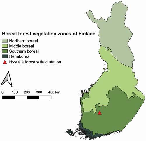
Our study site is located at Hyytiälä forestry field station (61°50'44”N, 24°17'10”E) in Juupajoki, Finland. The site belongs to the southern boreal forest zone (Figure 1), and the dominant overstorey species are Norway spruce (Picea abies), Scots pine (Pinus sylvestris) and birch (Betula pendula, Betula pubescens), either as mixed or single species stands. The study site is mostly covered by managed boreal forests growing on Podzolic soils, agricultural fields and wetlands. Different mosses, lichens and shrubs cover the forest floor. The growing season normally begins in early May and senescence in late August. The 30-year average annual mean temperature is 3.5 °C and annual precipitation is 711 mm (Pirinen et al. 2012). Elevation in the vicinity of the study site ranges from 135 to 198 m above sea level (Vastaranta et al. 2012).

Figure 1. Map of Finland and its boreal forest vegetation zones. Our study site is located in the vicinity of Hyytiälä forestry field station (61°50'44”N, 24°17'10”E) in the southern boreal forest zone.

2.2. Open forest data and test areas

In Finland, the forest resource inventory data is gathered by combining field measurements and remote sensing methods, namely airborne laser scanning (ALS) and aerial images. The inventory unit for which the forest data is originally estimated is a $16\mathrm{m}\times 16\mathrm{m}$ grid cell. Data for a grid cell is estimated with empirical imputation models that have been developed for each forest variable using the field measurements and the remote sensing data. A more detailed description of the laser scanning-based forest resource inventory is provided by Maltamo et al. (2011) and Holopainen et al. (2015). A summary of the inventory process used by the Finnish Forest Centre can be found in Halme, Pellikka and Mõttus (2019).

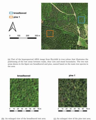
The forest resource inventory data is distributed as open data by the Finnish Forest Centre (Creative Commons Attribution 4.0 International, CC BY 4.0). We selected 20 homogeneous $70\mathrm{m}\times 70\mathrm{m}$ (0.49 ha) forest areas with different forest characteristics from the vicinity of the Hyytiälä forestry field station as our test areas (Table 1). We used the open forest data to select the test areas by locating clusters of grid cells for each of the three dominant overstorey species in Finnish boreal forests – pine, spruce, broadleaved (birch) – and additionally Siberian larch (Larix sibirica).

Table 1. Forest data for the test areas. The main tree species is indicated by the name of the test area. The coordinates in the centre point column correspond approximately to the centre of each test area

Test area	Centre	Basal	Stem	Mean	Crown
	point	area	count	height	diameter
	(lat, long)	(m^2 ha^–1)	(stems ha^–1)	(m)	(m)
pine 1	61°50'30”N, 24°18'29”E	19.8	921	17.1	3.4
pine 2	61°50'09”N, 24°20'50”E	23.4	643	21.0	4.0
pine 3	61°48'21”N, 24°20'29”E	20.7	556	20.5	4.1
pine 4	61°51'41”N, 24°16'14”E	21.9	795	18.3	3.3
pine 5	61°51'41”N, 24°15'22”E	18.1	1336	13.2	2.9
pine 6	61°51'25”N, 24°14'40”E	25.7	875	20.7	3.7
pine 7	61°49'24”N, 24°20'06”E	15.1	626	16.8	3.4
pine 8	61°49'29”N, 24°19'56”E	29.6	679	23.6	4.2
pine 9	61°51'37”N, 24°15'44”E	20.2	1449	13.6	2.8
spruce 1	61°49'28”N, 24°18'39”E	36.2	636	27.0	4.9
spruce 2	61°50'31”N, 24°16'16”E	22.5	1010	17.6	3.5
spruce 3	61°50'43”N, 24°18'01”E	34.8	632	26.1	4.9
spruce 4	61°49'34”N, 24°21'51”E	33.9	711	24.7	4.5
spruce 5	61°51'05”N, 24°17'01”E	32.3	616	26.2	4.8
spruce 6	61°49'35”N, 24°18'50”E	37.4	639	27.2	5.0
spruce 7	61°49'46”N, 24°20'31”E	33.8	896	22.6	4.0
spruce 8	61°50'26”N, 24°20'03”E	31.7	698	24.3	4.5
spruce 9	61°49'21”N, 24°22'00”E	32.0	669	24.2	4.3
larch	61°51'01”N, 24°18'04”E	19.4	669	20.7	5.6
broadleaved	61°50'36”N, 24°18'53”E	16.9	1070	18.2	4.5

We used the grid cell data from 2018 covering our study site, and averaged basal area, stem count, mean height and crown diameter from the grid cells overlaying our test areas (Table 1). Crown diameter was not included in the forest resource dataset. Hence, it was estimated for the grid cells using allometric regression models from tree height and diameter at breast height (DBH) used as independent variables. For pine and spruce, we used linear regressions developed by Rautiainen et al. (2008) for the same geographical area; for other species we used a model by Jakobsons (1970) developed for northern Sweden.

2.3. Remote sensing data

We used the remote sensing data by hyperspectral AISA imager (128 bands, 400–1000 nm, spatial resolution 0.7 m). The hyperspectral data was acquired under clear sky conditions on 15 June 2017 (08:38–09:12 UTC). During the data acquisition, the field of view of the AISA Eagle II hyperspectral scanner (Specim, Oulu, Finland) was 37.7°, the solar zenith angle changed from 42.3° to 40.3°, and the solar azimuth angle increased from 144° to 155°. Seven lines were flown 1 km above ground, approximately parallel to the direction of sunrays. The data was geolocated using the Atcor software package (ReSe Applications GmbH, Switzerland), converted to top-of-canopy reflectance with the Atcor package (ReSe Applications GmbH, Switzerland), resampled onto an orthogonal grid, and mosaicked. The processing chain is described in detail by Markiet, Hernández-Clemente and Mõttus (2017).

The test areas were clipped from the hyperspectral remote sensing image. The square-shaped test areas were 100 pixels in width (70 m), which was the maximum size that could be considered to provide enough data for a proper variogram analysis. We used the hyperspectral image to visually determine suitable forest areas as our test areas, i.e. areas without crossing roads and loggings (Figure 2). The homogeneity of the chosen test areas was tested by comparing the variance and sill from the sample variogram. If the sill did not equal the variance, the area was not considered homogeneous enough. The homogeneity was studied using spectral data from near infrared (NIR) band ($\lambda =835$ nm), which should provide more spatial variability than spectral bands recorded in the visible part of the spectrum (Chavez 1992).

Figure 2. The hyperspectral AISA image was used to determine suitable forest areas for our test areas, which had a size of $70\mathrm{m}\times 70\mathrm{m}$.

2.4. Simulated images

In addition to real data, we used seven simulated forest images based on individual tree data to test the validity of the hypothesis in actual boreal forests. The synthetic images were created using a Monte Carlo ray tracing model, where the paths of photons are traced within a 3D canopy until they either get absorbed or exit through the top of the canopy. Our model uses cyclic boundary conditions, where a photon exiting from one side of the canopy re-enters from the opposite side.

Tree data used in the Monte Carlo simulations was originally collected in the vicinity of Hyytiälä forestry field station. There are numerous permanent plots in Hyytiälä for which trees have been accurately positioned and measured (Hovi et al. 2016). The positioning of the trees was initially carried out using a total station or a photogrammetric method, which applies the monoplotting principle and airborne LiDAR data (Korpela, Tuomola and Välimäki 2007; Korpela et al. 2010).

The tree data used in the simulations belonged to seven different plots. The plots were measured during the summer months of 2013–2015. The used plots included trees that were re-measured during summer 2013 and 2014 and trees that were accurately mapped and measured for the first time in summer 2015. There were several variables measured for each located tree during the field measurement campaigns. The variables relevant for this study were DBH and tree species. In addition, tree height, crown base height and a few other tree growth-related measurements were carried out for a set of sample trees during the campaigns.

We calculated missing tree heights with the Näslund model (Näslund 1936; Siipilehto and Kangas 2015) using the sample trees. For trees (typically suppressed trees) without DBH values but where tree height was available, the Näslund model was inverted for DBH. Tree leaf area used in the simulations was calculated using dry leaf weight (Repola 2008, 2009) and specific leaf area, similarly to Majasalmi et al. (2013).

The tree crowns were modelled as ellipsoids of turbid medium, whose scattering elements corresponded to randomly oriented bi-Lambertian leaves. We used birch leaf transmittance and reflectance data measured by Hovi, Raitio and Rautiainen (2017) regardless of the actual species of the modelled tree, as we were only investigating the spatial correlation distances and not the level of contrast in the images. The solar azimuth angle was set to 150° and the solar zenith angle to 41° with the sensor at zenith. The simulated images had the same pixel size and dimensions as the test areas.

We simulated two scenarios (Table 2) for each plot: (1) a canopy with a completely absorbing understorey and the direct-to-global irradiance ratio was equal to one, i.e. direct solar sunlight was the only source of irradiance (the so-called ‘ideal’ scenario), and (2) a canopy with an understorey with non-zero reflectance and diffuse-sky irradiance was included (the so-called ‘realistic’ scenario). Understorey reflectance measurements by Rautiainen et al. (2011) were used in the realistic scenario. The direct-to-global irradiance ratio was calculated with the 6S atmospheric radiative transfer model (Vermote et al. 1997) using the same input parameters as Mõttus et al. (2015).

Table 2. The values of the canopy spectral variables for the two scenarios used in the Monte Carlo simulations. The used wavelength was 835 nm

	Understorey reflectance	Leaf reflectance	Leaf transmittance	Direct-to-global irradiance ratio
ideal	0.0	0.476	0.426	1.0
realistic	0.283	0.476	0.426	0.883

3. Methods

3.1. Variogram

3.1.1. Sample variogram computation

The sample variogram is created with a two-step procedure where we first compute a scatterplot of squared sample value differences, i.e. the variogram cloud, and secondly group the points of the cloud into distance classes (Figure 3).

Figure 3. Flowchart of the used methodology. The same methods were also used for the simulated images.

If we have $n$ samples at locations $x_1,\dots ,x_n$, the variogram cloud is the scatterplot of all squared sample value differences $s_{\mathrm{i}\mathrm{j}}=[z(x_i)-z(x_j){]}^2$ as a function of distance d(x_i, x_j). The sample variogram is created from the variogram cloud by binning the points into successive distance classes, for which we used a bin size of 0.5 m. For each distinct distance class, we computed the gammavariance (Bachmaier and Backes 2011) as half of the sample average of all squared differences (Equation 1(1) $\hat{\gamma }(d)=\frac{1}{2}\frac{1}{N(d)}\sum _{\parallel x_i-x_j\parallel \approx d}[z(x_i)-z(x_j){]}^2,$(1) ),

(1) $\hat{\gamma }(d)=\frac{1}{2}\frac{1}{N(d)}\sum _{\parallel x_i-x_j\parallel \approx d}[z(x_i)-z(x_j){]}^2,$(1)

where $N(d)$ is the number of data pairs separated by a distance of approximately $d$.

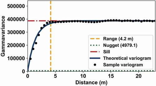
The gammavariance increases with distance, until the increase flattens out. This distance where the sample variogram first flattens out is known as the range (Figure 4), which is the measure of spatial dependency and it corresponds to the decorrelation distance. Sample locations separated by distances closer than the range are spatially autocorrelated, whilst locations further apart than the range are not. The gammavariance corresponding to the range is called the sill (Figure 4), which describes the data variability. For second-order stationary processes (e.g. homogeneous forest stand), the sill equals the variance. The gammavariance at $d=0$ is known as the nugget (or nugget variance), which depicts the small-scale variability of the data.

Figure 4. Variogram analysis for test area ‘pine 8’ ($\lambda =835$ nm).

3.1.2. Theoretical variogram fitting

We fitted the gammavariances from the sample variogram with the exponential model

(2) $\gamma (d)={\sigma }^2(1-e^{-\frac{3d}{r}}),$(2)

where $d$ is distance, $r$ is range and ${\sigma }^2$ is sill (i.e. variance).

The exponential model provided good fit in tests (data not shown), and it suited our purpose whereby we wanted to avoid any visual inspection when determining range r and nugget n.

3.2. Amplitude spectrum

3.2.1. Averaged amplitude spectrum

We performed two-dimensional discrete fast Fourier transform on a single band of an image ($\lambda =835$ nm). The obtained amplitude spectrum $S(p,q)$ of an $N\times N$ image is given by

(3) $S(p,q)=\frac{\left|F(p,q)\right|}{N^2},$(3)

where $F$ is the Fourier transform and $(p,q)$ are indices in the frequency domain, i.e. spatial frequencies and equivalent to $(x,y)$ in the spatial domain. The greatest amplitude in the amplitude spectrum corresponds to zero frequency which, by convention, is typically defined as the centre point of the spectrum (Field 1987).

Finally, we averaged the Fourier amplitude spectrum over all orientations as a function of spatial frequency ($f$). Only frequencies above the zero frequency and below the highest resolvable Nyquist frequency ($N/2$) were included: $1\le f\le N/2$.

3.2.2. Structure of averaged amplitude spectrum

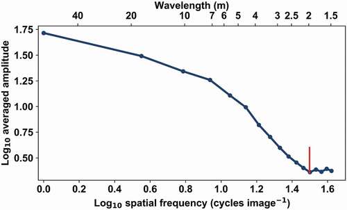
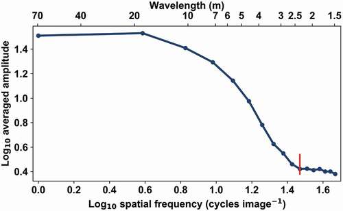
We studied the averaged amplitude spectra of our test areas and found structures that correlated with forest characteristics. We used a point where the average amplitude flattens out in the high frequencies to quantify the structure in the averaged amplitude spectrum of a test area. We designated the point as the breaking point (Figure 6).

Figure 5. Relationships between the allometric mean crown diameters of the test areas and the estimations from (a) variogram and (b) amplitude spectrum analyses. The metrics used in the graphs are Pearson correlation coefficient (r), root-mean-square error (RMSE), and relative root-mean-square error (rRMSE).

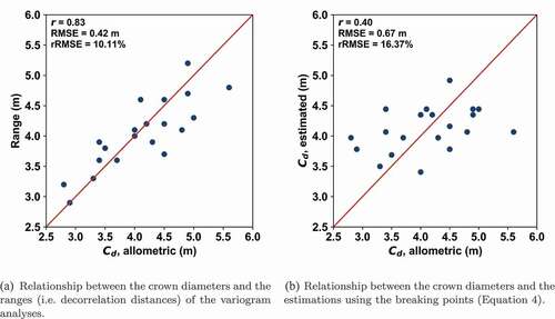
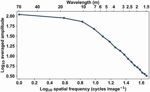
Figure 6. Averaged amplitude spectrum of measured reflectance (λ = 835 nm) for the test area ‘spruce 6’ in log-log coordinates. The red line corresponds to the visually located breaking point at 2.35 m.

The breaking point $P_{bp}$ was gathered for each test area in metres. We assumed that it is a parameter characterizing the geometric properties of a crown and looked for a linear relationship between the crown diameter $C_d$ and the breaking point $P_{bp}$ as

(4) $C_d=K_{bp}{P}_{bp},$(4)

where $K_{bp}$ is a proportionality coefficient.

4. Results

4.1. Variograms

The spatial variability and dependency within our test areas were studied using the variograms (Figure 4). We focused only on the range, because the nugget effect was small (data not shown), i.e. $<3\mathrm{\%}$ and in most cases $<2\mathrm{\%}$ of the sill (i.e. variance).

The correlation between the ranges and the mean crown diameter was good (Pearson correlation $r=0.83$). The relative root-mean-square error was approximately $10\mathrm{\%}$ (Figure 5). In general, the ranges were of similar order of magnitude between all test areas. They ranged from 3.6 m to 5.2 m. The largest absolute error for estimating mean crown diameter with range was 0.8 m for ‘broadleaved’ and ‘larch’ test areas. Other less accurate estimations were obtained for ‘spruce 5’ and ‘spruce 6’ (absolute errors 0.7 m). The absolute errors for rest of the test areas were all less than or equal to half a metre. The obtained estimation errors had no clear connection to any of the forest characteristics (Table 3).

Table 3. Connection between the absolute estimation errors of the variogram analyses and the forest characteristics of our test areas (Table 1)

Forest variable	Basal area (m^2 ha^−1)	Stem count (stems ha^−1)	Mean height (m)	Crown diameter (m)
Pearson correlation coefficient (r)	-0.10	-0.15	0.13	0.50

4.2. Amplitude spectra

The averaged amplitude spectra of our test areas were also used to study the spatial variability and structure. In the high frequencies of the amplitude spectra of our test areas, we detected decreasing average amplitudes and small horizontal plateaus. For some test areas the plateau was very explicit (e.g. for test area ‘spruce 6’ in Figure 6) and for some others it was more ambiguous (data not shown). We referred to the point between the decreasing slope of amplitudes and the plateau as the breaking point $P_{bp}$ (in metres). We gathered the breaking points for each of our test areas and used them to estimate mean crown diameters using Equation 4(4) $C_d=K_{bp}{P}_{bp},$(4) . We observed that the most accurate estimations are obtained with $K_{bp}=1.89$. The absolute errors of the mean crown diameter estimations ranged from 0.1 m to 1.5 m. The largest absolute error was obtained for test area ‘larch’ (1.5 m). Large absolute errors were also obtained for ‘pine 9’ (1.2 m), ‘pine 1’ (1.0 m) and ‘pine 5’ (0.9 m). Out of all the 20 estimations, 10 had an accuracy under or equal to half a metre and 16 had an accuracy under or equal to 0.7 m. It should be noted that the errors include the inaccuracy of the allometric regression models, i.e. the reference values.

A relatively weak correlation existed (Pearson correlation $r=0.40$) between the mean crown diameter and the estimations utilizing the breaking point (Figure 5). The relative root-mean-square error was approximately $16\mathrm{\%}$.

4.3. Simulated forest images

We created two different radiation scenarios in boreal forests using the Monte Carlo simulations: an ideal and a realistic scenario (Figure 7). The ranges of variograms, which predicted the mean crown diameters, were quite similar for both scenarios (Table 4).

Figure 7. Monte Carlo simulated forest of Plot 1 (‘realistic’ scenario). The simulated forest can be seen at the centre of the image with spatial dimensions of 70 m $\times$ 70 m. Measured reflectance data by the hyperspectral AISA imager was used as visualisation on the background. The used wavelength for the spectral data was 835 nm. Note that we used birch leaf spectrum for all modelled trees, whilst most of the real trees in the AISA image are conifers with lower 835 nm reflectance. We also traced $2\times {10}^9$ photons to ensure low Monte Carlo noise in the images.

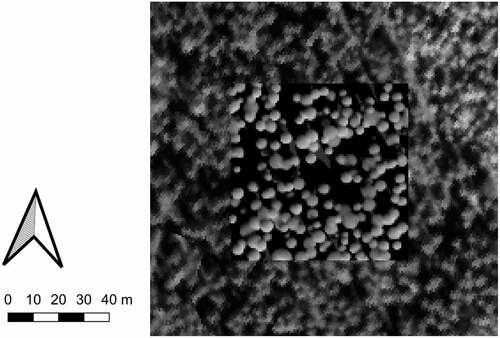
Table 4. Ranges of the variograms of the simulated forest images. ‘Ideal’ and ‘realistic’ describe the used simulation scenarios (Table 2)

Plot name	Crown	Range,	Range,
	diameter (m)	ideal (m)	realistic (m)
Plot 1	4.6	4.5	4.9
Plot 2	3.7	5.7	5.6
Plot 3	4.1	4.3	4.4
Plot 4	5.2	5.2	4.6
Plot 5	3.5	3.2	3.4
Plot 6	4.8	5.4	5.3
Plot 7	5.4	5.6	5.5

Simulated ‘Plot 2’ forests were clear outliers, as both ideal and realistic forests had an inaccurate estimate (absolute errors 2.0 m and 1.9 m, respectively). In addition, simulated ‘Plot 6’ forest had slightly weaker estimation accuracy than the others, since with ideal and realistic forests the absolute errors were 0.6 m and 0.5 m, respectively. The estimation for realistic ‘Plot 4’ forest also had larger absolute error compared to others (0.6 m). Absolute errors for the other simulated forests were all less than or equal to 0.3 m. In general, there were more overestimations than underestimations. Relative root-mean-square error was $18.0\mathrm{\%}$ for ideal and $17.8\mathrm{\%}$ for realistic forests. Ignoring the outlier, i.e. ‘Plot 2’, decreased the relative root-mean-square errors to $6.5\mathrm{\%}$ and $8.0\mathrm{\%}$, respectively.

The amplitude spectrum analysis, as introduced in the present paper, did not apply to the simulated images. The averaged amplitude spectra did not show any structure in the high spatial frequencies (Figure 8). Each spectrum of the 14 simulated forests exhibited a clear linear decrease in the higher frequencies (approximately after 10 m).

Figure 8. Averaged amplitude spectrum of simulated reflectance for ideal ‘Plot 4’. The spectrum does not show any clear structure in the high frequencies. The estimation accuracy for the mean crown diameter using variogram was 0.0 m for the same simulated image (Table 4).

5. Discussion

5.1. Information content of very-high-resolution imagery

In this study, we assessed the spatial variability in Finnish boreal forests using very-high-resolution imagery. We used two different approaches to study the second-order statistics of reflectance factors: a variogram, which is a central geostatistical method, and an averaged amplitude spectrum that we obtained from a two-dimensional Fourier transform. Several past studies had demonstrated the use of the variogram approach, whereas the amplitude spectrum approach, as it is presented in this paper, was a novel approach to explore the spatial structure of a forested area.

The very-high-resolution data suited the variogram and amplitude spectrum analyses well, and we retrieved information on forest characteristics successfully. We were able to study spatial variability and investigate structural information on Finnish boreal forests at the canopy level using both approaches.

The variogram analysis worked well with the used imagery, and we estimated mean crown diameter with reasonable accuracy. The estimation results using variograms were consistent with what past studies had reported. The amplitude spectrum analysis was less successful since we were not able to achieve similar estimation accuracy for crown diameter as with variograms. Further, the amplitude spectrum approach did not apply to the simulated forest images used in the study, which ignored within-crown distribution of foliage.

5.2. Spatial variability expressed by variograms

When applying geostatistics, such as variograms, to remote sensing image analysis, it is important to realize when stationarity is a reasonable assumption. In general, it can be debated whether it is fair to assume and apply stationarity to real-world processes when using geostatistical techniques (van der Meer 2012). Typical geostatistical assumptions may not hold for vast remote sensing image scenes but locally and on smaller areas the assumptions can be reasoned. In forest ecosystems, variograms should be computed from relatively large areas because of the complex texture of forests (Zawadzki et al. 2005). At the same time, unnecessarily large forest areas may become heterogeneous, which influences the correlation structure, and overly small forest areas restrain the computation of variograms. The scale at which the variogram is applicable needs to be determined from a test of stationarity.

In Finland, forests are managed at stand level. Stands are aggregations of trees that are sufficiently uniform in species composition, size, arrangement and age, and they are delineated subjectively to be relatively homogeneous. Furthermore, forest stands in Finland are typically heavily homogenized as a result of intensive silviculture. In Finnish boreal forests, however, the understorey can have a major effect on the homogeneity. Due to gaps in the canopy, local differences in reflectance and transmittance within a stand are inevitable. The structure and optical properties of the green forest floor make a considerable contribution to the reflected and measured signal. Regardless of this, it is still possible to find spatially homogeneous forest patches within the stands. Considering the above, the forests of our test areas were selected to be sufficiently large to allow the variogram computation and they had been tested to be as homogeneous as possible, i.e. dominant overstorey species existed and the sill equalled the variance as it is assumed for second-order stationary processes.

Our results from variograms were consistent with what previous studies had reported, as the range exhibited a clear positive correlation with the mean crown diameter (Pearson correlation $r=0.83$) and the relative root-mean-square error was approximately $10\mathrm{\%}$ (RMSE $=0.42$ m), which can be regarded as reasonable accuracy when considering typical crown diameters in Finnish boreal forests. St-Onge and Cavayas (1997) estimated stand crown diameter with a median error of 0.3 m. Suhardiman, Tsuyuki and Setiawan (2016) predicted mangrove forest crown diameter with relatively low error ($6.19\mathrm{\%}$ and less than 0.5 m) using the range. Feng, Li and Tokola (2010) were able to estimate mean crown diameter in Chinese pine and poplar plantations with errors ranging from approximately $4\mathrm{\%}$ to $18\mathrm{\%}$ for very high ($\sim 2000$ stems ha⁻¹) and moderate ($\sim 800$ stems ha⁻¹) canopy densities, respectively. Based on their study, the estimation accuracy decreased with decreasing density, which was not evident in our study. Further, Feng, Li and Tokola (2010) found that estimations were better in stands where variation in crown size is low. In our study, this could be checked only for the simulated images for which we had individual tree data available. However, we did not notice any effect of the crown size variation.

To the best of our knowledge, this is the first study to use variograms to assess the spatial variability within Finnish forests using very-high-resolution hyperspectral remote sensing data and Monte Carlo simulated images. The reference values of crown diameter for the simulated images had good accuracy and reliability. To this end, the accurate estimations for the simulated images also prove that the range can be used to estimate mean crown diameter, and that canopy structure affects the spatial variability of reflectance factors in Finnish boreal forests together with mutual tree shading and self-shading.

Differences in crown diameter estimations in terms of tree species could be examined reliably only for pine and spruce, because we only had a single test area for broadleaved and larch. In general, estimations for pine were more accurate than for spruce. We had nine test areas for both species, but we achieved estimation errors below 0.1 m only for pine (for four different test areas). The smallest error for spruce was 0.1 m (for two test areas). The largest errors for pine and spruce were 0.5 m and 0.7 m, respectively. In terms of estimations for pine, we had only one underestimation and four overestimations, whereas for spruce we had five underestimations and four overestimations. The median absolute error for pine and spruce test areas were 0.1 m and 0.3 m, respectively. The allometric linear regressions, which were used to compute the reference values for crown diameter using the averaged grid cell data, were more accurate for pine in the study by Rautiainen et al. (2008) in which the regressions were originally presented. Considering this, the more accurate estimations for pine seemed reasonable.

5.3. Spatial information exhibited by amplitude spectra

The Fourier-transformed amplitude spectra of our test areas consisted of two plateaus and a transition between them (Figure 6). The plateaus have spectra of white noise at high and low frequencies (wavelength below 2.5 m and above 20 m, respectively). This indicates that the canopy has no clear structure at the corresponding scales. At the low end of the spectrum, this indicates a regular homogeneous forest, and at higher frequencies, no regular structural elements of sizes larger than the inverse of Nyquist frequency – in our case, 1.4 m. This is in line with the theoretical expectations.

A lack of a point of maximum curvature at high frequencies in the Fourier-transformed simulated images requires further investigation, especially considering that crown size information could be retrieved from them using variogram analysis. In simulated images, crowns were simulated as objects with sharp edges, filled continuously with reflective matter. The AISA images, on the other hand, were formed by leaves and other plant elements in varying shade (i.e. penumbra) and smoothed by the point spread function (PSF) of the sensor. A lack of a clear indicator of crown size in the latter could be explained by the masking of the signal by high-frequency components created by sharp crown edges (Figure 7). As we ignored the absolute amplitude of the spectrum and only investigated its dependence on frequency, using a different, well-defined spectrum makes sense. However, together with unrealistic representation of crown edges, it did increase the sharp contrasts with the dark shadows. In our opinion, ignoring the sensor PSF had an effect on the interpretation of the Fourier spectrum. Whilst the PSF was constant for the whole image, the shapes of the curves varied between the test areas, although we could not fully explain the variation.

The problem with the amplitude spectra of the simulated images predicts difficulties in simulating the spatial statistics with forest reflectance models, assuming the scene consists of geometric crown shapes with sharp edges. A more feasible approach would be the retrieval of crown diameter from very-high-resolution imagery as described in the present paper and using forest reflectance models to retrieve other forest variables utilizing the spatially averaged reflectance spectra of a forest. Alternatively, the retrieved crown diameter could be used to constrain reflectance model inversion.

In the amplitude spectrum analysis, as presented in this paper, the determination of the breaking point $P_{bp}$ is done visually, which can be ambiguous. For the future, an automated detection of $P_{bp}$ would be an advisable option. Nevertheless, we considered the visual determination performed in this study to be sufficient and successful, as we also managed to estimate mean crown diameters for heterogeneous and non-stationary forests (Appendix A). We hypothesized that the averaged amplitude spectra could be applicable also to heterogeneous, partly logged, forest areas where variograms do not work. To check this, we created five additional test regions, similar to our original test areas. We observed that the averaged amplitude spectrum detects the most important structure from the partly logged image, i.e. the forest, and gives less value for the barren deforested area. The use of the partly logged regions substantiated the applicability of the proposed cooperative use of the averaged amplitude spectra and the breaking points when estimating mean crown diameter.

6. Conclusions

We estimated the mean crown diameter and investigated the spatial variability in Finnish boreal forests using the second-order statistics of reflectance factors in very-high-resolution imagery (airborne hyperspectral data and simulated images). The second-order statistics were retrieved using variograms and Fourier amplitude spectra.

Variograms, which are an established geostatistical method, estimated mean crown diameters with reasonable accuracy for the hyperspectral and simulated data, which is in line with past studies. The wider applicability of the variogram is limited by non-stationarity over large areas. Forest ecosystems typically exhibit higher variability than most other remote sensing targets. Therefore, any heterogeneity should be minimized, as variograms only apply on smaller scales to spatially homogeneous forest patches. The test areas used in this study were selected after careful consideration. The Fourier amplitude spectrum approach presented in this study is a novel approach to explore the spatial structure of a forest stand. The Fourier spectrum yielded weaker accuracies than the variogram when estimating mean crown diameter but was applicable also to heterogeneous and non-stationary forests. The results are encouraging, and this method has the potential to study spatial variability within a forested area instead of using only the mean reflectance to characterize the structural properties. For the simulated images, however, the amplitude spectra did not work. Further research would be required to explain this discrepancy.

Our results highlight the need for high spatial resolution when there is an interest in studying variability within a forest stand. The high spatial resolution enabled the retrieval of mean crown diameter from the used imagery. This study contributes to retrieval of more detailed forest information from very-high-resolution imagery in boreal forests.

Acknowledgements

We would like to acknowledge assistance from the University of Helsinki and Ilkka Korpela for providing us with the field measured tree data from Hyytiälä.

Disclosure statement

No potential conflict of interest was reported by the author(s).

Additional information

Funding

This work was supported by the Academy of Finland under Grant [317387].

Appendix A.

Analysis of heterogeneous areas

We hypothesized that the averaged Fourier amplitude spectrum approach could also be applicable to heterogeneous areas where variograms are not applicable. To check this, we created additional test regions (Figure A1), and tested whether we could use the averaged amplitude spectrum to also retrieve mean crown diameter from an image that is partly covered by a deforested area.

The variogram did not work, because the image was not homogeneous enough (Figure A2). The averaged amplitude spectrum, however, detected the most important spatial structure from the image, i.e. the forest, and gave less value for the barren deforested area. The averaged amplitude spectrum exhibited structure similar to the other test areas used in the study. We used Equation 4(4) $C_d=K_{bp}{P}_{bp},$(4) to calculate the estimation for the mean crown diameter using the breaking point (Figure A3). The estimation error for the region presented here was 0.1 m.

The use of the partly logged test regions substantiated the applicability of the proposed cooperative use of the averaged amplitude spectra and the breaking points when estimating mean crown diameter in Finnish boreal forests. Furthermore, this method proved itself suitable for analysing inner variations of a forest (stand), and it can be considered as a new potential approach for exploring the spatial variability within the stand instead of using only the mean reflectance to characterize the structural properties.

Figure A1. One of the additional test regions, which were used to test the hypothesis. Mean crown diameter for the forested area was 3.6 m.

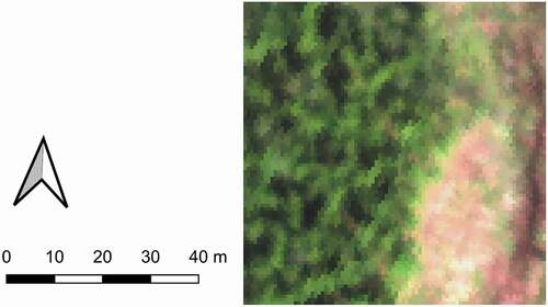
Figure A2. Variogram analysis for one of the additional test regions ($\lambda =835$ nm). The analysis did not succeed for the partly logged forest area.

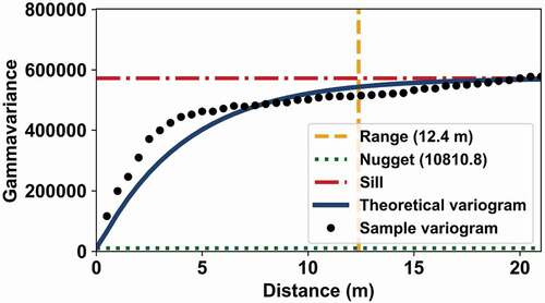
Figure A3. Averaged amplitude spectrum of measured reflectance ($\lambda =835$ nm) for one of the additional test regions in log-log coordinates. The red line corresponds to the visually located breaking point at 1.98 m.

References

- Bachmaier, M. and M. Backes. 2011. “Variogram or Semivariogram? Variance or Semivariance? Allan Variance or Introducing a New Term?” Mathematical Geosciences 43 (6): 735–740. doi:https://doi.org/10.1007/s11004-011-9348-3.
- Barbier, N., P. Couteron, J. Lejoly, V. Deblauwe, and O. Lejeune. 2006. “Self-Organized Vegetation Patterning as a Fingerprint of Climate and Human Impact on Semi-Arid Ecosystems.” The Journal of Ecology 94 (3): 537–547. doi:https://doi.org/10.1111/j.1365-2745.2006.01126.x.
- Bonan, G. B. 2008. “Forests and Climate Change: Forcings, Feedbacks, and the Climate Benefits of Forests.” Science 320 (5882): 1444–1449. doi:https://doi.org/10.1126/science.1155121.
- Chavez, P. S. 1992. “Comparison of Spatial Variability in Visible and Near-Infrared Spectral Images.” Photogrammetric Engineering and Remote Sensing 58 (7): 957–964.
- Cohen, W. B., T. A. Spies, and G. A. Bradshaw. 1990. “Semivariograms of Digital Imagery for Analysis of Conifer Canopy Structure.” Remote Sensing of Environment 34 (3): 167–178. doi:https://doi.org/10.1016/0034-4257(90)90066-U.
- Couteron, P. 2002. “Quantifying Change in Patterned Semi-Arid Vegetation by Fourier Analysis of Digitized Aerial Photographs.” International Journal of Remote Sensing 23 (17): 3407–3425. doi:https://doi.org/10.1080/01431160110107699.
- Couteron, P., N. Barbier, and D. Gautier. 2006. “Textural Ordination Based on Fourier Spectral Decomposition: A Method to Analyze and Compare Landscape Patterns.” Landscape Ecology 21 (4): 555–567. doi:https://doi.org/10.1007/s10980-005-2166-6.
- Couteron, P., R. Pelissier, E. Nicolini, and D. Paget. 2005. “Predicting Tropical Forest Stand Structure Parameters from Fourier Transform of Very High-Resolution Remotely Sensed Canopy Images.” The Journal of Applied Ecology 42 (6): 1121–1128. doi:https://doi.org/10.1111/j.1365-2664.2005.01097.x.
- Curran, P. J. 1988. “The Semivariogram in Remote Sensing: An Introduction.” Remote Sensing of Environment 24 (3): 493–507. doi:https://doi.org/10.1016/0034-4257(88)90021-1.
- Feng, Y., Z. Li, and T. Tokola. 2010. “Estimation of Stand Mean Crown Diameter from High-Spatial-Resolution Imagery Based on a Geostatistical Method.” International Journal of Remote Sensing 31 (2): 363–378. doi:https://doi.org/10.1080/01431160902887867.
- Field, D. J. 1987. “Relations Between the Statistics of Natural Images and the Response Properties of Cortical Cells.” Journal of the Optical Society of America A 4 (12): 2379–2394. doi:https://doi.org/10.1364/JOSAA.4.002379.
- Gauthier, S., P. Bernier, T. Kuuluvainen, A. Z. Shvidenko, and D. G. Schepaschenko. 2015. “Boreal Forest Health and Global Change.” Science 349 (6250): 819–822. doi:https://doi.org/10.1126/science.aaa9092.
- Halme, E., P. Pellikka, and M. Mõttus. 2019. “Utility of Hyperspectral Compared to Multispectral Remote Sensing Data in Estimating Forest Biomass and Structure Variables in Finnish Boreal Forest.” International Journal of Applied Earth Observation and Geoinformation 83: 101942. doi:https://doi.org/10.1016/j.jag.2019.101942.
- Holopainen, M., T. Tokola, M. Vastaranta, J. Heikkilä, H. Huitu, R. Laamanen, and P. Alho. 2015. ”Metsätalouteen, maatalouteen ja vesistöihin liittyviä paikka-tietosovelluksia.” In Geoinformatiikka luonnonvarojen hallinnassa, University of Helsinki Department of Forest Sciences Publications 7, Chap. 14, pp. 121–130 http://hdl.handle.net/10138/166765. Finland: Department of Forest Sciences, University of Helsinki. [In Finnish].
- Hovi, A., L. Korhonen, J. Vauhkonen, and I. Korpela. 2016. “LiDAR Waveform Features for Tree Species Classification and Their Sensitivity to Tree- and Acquisition Related Parameters.” Remote Sensing of Environment 173: 224–237. doi:https://doi.org/10.1016/j.rse.2015.08.019.
- Hovi, A., P. Raitio, and M. Rautiainen. 2017. “A Spectral Analysis of 25 Boreal Tree Species.” Silva Fennica 51 (4). doi:https://doi.org/10.14214/sf.7753.
- Jakobsons, A. 1970. “The Correlation Between the Diameter of Tree Crown and Other Tree Factors — Mainly the Breastheight Diameter.” In Vol. 14 of Research Notes. Sweden: Department of Forest, Survey, Royal College of Forestry.
- Korpela, I., H. O. Ørka, M. Maltamo, T. Tokola, and J. Hyyppä. 2010. “Tree Species Classification Using Airborne LiDAR – Effects of Stand and Tree Parameters, Downsizing of Training Set, Intensity Normalization, and Sensor Type.” Silva Fennica 44 (2): 319–339. doi:https://doi.org/10.14214/sf.156.
- Korpela, I., T. Tuomola, and E. Välimäki. 2007. “Mapping Forest Plots: An Efficient Method Combining Photogrammetry and Field Triangulation.” Silva Fennica 41 (3): 457–469. doi:https://doi.org/10.14214/sf.283.
- Lévesque, J. and D. J. King. 1999. “Airborne Digital Camera Image Semivariance for Evaluation of Forest Structural Damage at an Acid Mine Site.” Remote Sensing of Environment 68 (2): 112–124. doi:https://doi.org/10.1016/S0034-4257(98)00104-7.
- Majasalmi, T., M. Rautiainen, P. Stenberg, and P. Lukeš. 2013. “An Assessment of Ground Reference Methods for Estimating LAI of Boreal Forests.” Forest Ecology and Management 292: 10–18. doi:https://doi.org/10.1016/j.foreco.2012.12.017.
- Maltamo, M., P. Packalén, E. Kallio, J. Kangas, J. Uuttera, and J. Heikkilä. 2011. “Airborne Laser Scanning Based Stand Level Management Inventory in Finland.” In Proceedings of SilviLaser 2011, 11th International Conference on LiDAR Applications for Assessing Forest Ecosystems, University of Tasmania, Australia, 16-20 October 2011, 1–10 . Conference Secretariat. http://www.iufro.org/download/file/8239/5065/40205-silvilaser2011.pdf
- Markiet, V., R. Hernández-Clemente, and M. Mõttus. 2017. “Spectral Similarity and PRI Variations for a Boreal Forest Stand Using Multi-Angular Airborne Imagery.” Remote Sensing 9 (10): 1005. doi:https://doi.org/10.3390/rs9101005.
- Mõttus, M., T. L. H. Takala, P. Stenberg, Y. Knyazikhin, B. Yang, and T. Nilson. 2015. “Diffuse Sky Radiation Influences the Relationship Between Canopy PRI and Shadow Fraction.” ISPRS Journal of Photogrammetry and Remote Sensing 105 (3): 54–60. doi:https://doi.org/10.1016/j.isprsjprs.2015.03.012.
- Muinonen, E., M. Maltamo, H. Hyppänen, and V. Vainikainen. 2001. “Forest Stand Characteristics Estimation Using a Most Similar Neighbor Approach and Image Spatial Structure Information.” Remote Sensing of Environment 78 (3): 223–228. doi:https://doi.org/10.1016/S0034-4257(01)00220-6.
- Näslund, M. 1936. ”Skogsförsöksanstaltens gallringsförsök i tallskog.” In Meddelanden från Statens Skogsförsöksanstalt 29 (Stockholm: Statens skogsförsöksanstalt. Publisher), p. 169. [In Swedish].
- Nilson, T. 1999. “Inversion of Gap Frequency Data in Forest Stands.” Agricultural and Forest Meteorology 98–99: 437–448. doi:https://doi.org/10.1016/S0168-1923(99)00114-8.
- Pan, Y., R. A. Birdsey, O. L. Phillips, and R. B. Jackson. 2013. “The Structure, Distribution, and Biomass of the World’s Forests.” Annual Review of Ecology, Evolution, and Systematics 44 (1): 593–622. doi:https://doi.org/10.1146/annurev-ecolsys-110512-135914.
- Pirinen, P., H. Simola, J. Aalto, J. P. Kaukoranta, P. Karlsson, and R. Ruuhela. 2012. ”Tilastoja Suomen ilmastosta 1981–2010.” In Vol. 1 of Reports 2012. Finnish Meteorological Institute 32–33. http://hdl.handle.net/10138/35880. [In Finnish].
- Poso, S., T. Häme, and R. Paananen. 1984. “A Method for Estimating the Stand Characteristics of a Forest Compartment Using Satellite Imagery.” Silva Fennica 18 (3): 261–292. doi:https://doi.org/10.14214/sf.a15398.
- Proisy, C., P. Couteron, and F. Fromard. 2007. “Predicting and Mapping Mangrove Biomass from Canopy Grain Analysis Using Fourier-Based Textural Ordination of IKONOS Images.” Remote Sensing of Environment 109 (3): 379–392. doi:https://doi.org/10.1016/j.rse.2007.01.009.
- Rautiainen, M., M. Mõttus, J. Heiskanen, A. Akujärvi, T. Majasalmi, and P. Stenberg. 2011. “Seasonal Reflectance Dynamics of Common Understory Types in a Northern European Boreal Forest.” Remote Sensing of Environment 115 (12): 3020–3028. doi:https://doi.org/10.1016/j.rse.2011.06.005.
- Rautiainen, M., M. Mõttus, P. Stenberg, and S. Ervasti. 2008. “Crown Envelope Shape Measurements and Models.” Silva Fennica 42 (1): 19–33. doi:https://doi.org/10.14214/sf.261.
- Renshaw, E. and E. D. Ford. 1983. “The Interpretation of Process from Pattern Using Two-Dimensional Spectral Analysis: Methods and Problems of Interpretation.” Journal of the Royal Statistical Society. Series C (Applied Statistics) 32 (1): 51–63.
- Repola, J. 2008. “Biomass Equations for Birch in Finland.” Silva Fennica 42 (4): 605–624. doi:https://doi.org/10.14214/sf.236.
- Repola, J. 2009. “Biomass Equations for Scots Pine and Norway Spruce in Finland.” Silva Fennica 43 (4): 625–647. doi:https://doi.org/10.14214/sf.184.
- Siipilehto, J. and A. Kangas. 2015. ”Näslundin pituuskäyrä ja siihen perustuvia malleja läpimitan ja pituuden välisestä riippuvuudesta suomalaisissa talousmetsissä.” Metsätieteen aikakauskirja 4: 215–236 https://www.metsatieteenaikakauskirja.fi/pdf/article6584.pdf. [In Finnish].
- Song, C. 2007. “Estimating Tree Crown Size with Spatial Information of High Resolution Optical Remotely Sensed Imagery.” International Journal of Remote Sensing 28 (15): 3305–3322. doi:https://doi.org/10.1080/01431160600993413.
- St-Onge, B. A. and F. Cavayas. 1997. “Automated Forest Structure Mapping from High Resolution Imagery Based on Directional Semivariogram Estimates.” Remote Sensing of Environment 61 (1): 82–95. doi:https://doi.org/10.1016/S0034-4257(96)00242-8.
- Stenberg, P., M. Mõttus, and M. Rautiainen. 2008. Modeling the Spectral Signature of Forests: Application of Remote Sensing Models to Coniferous Canopies, pp. 147–171. Dordrecht: Springer Netherlands.
- Suhardiman, A., S. Tsuyuki, and Y. Setiawan. 2016. ”Estimating Mean Tree Crown Diameter of Mangrove Stands Using Aerial Photo.” Procedia Environmental Sciences 33: 416–427 . 2nd International Symposium on LAPAN-IPB Satellite (LISAT) for Food Security and Environmental Monitoring. doi:https://doi.org/10.1016/j.proenv.2016.03.092.
- Treitz, P. 2001. “Variogram Analysis of High Spatial Resolution Remote Sensing Data: An Examination of Boreal Forest Ecosystems.” International Journal of Remote Sensing 22 (18): 3895–3900. doi:https://doi.org/10.1080/01431160110069890.
- Treitz, P. and P. Howarth. 2000. “High Spatial Resolution Remote Sensing Data for Forest Ecosystem Classification: An Examination of Spatial Scale.” Remote Sensing of Environment 72 (3): 268–289. doi:https://doi.org/10.1016/S0034-4257(99)00098-X.
- van der Meer, F. 2012. “Remote-Sensing Image Analysis and Geostatistics.” International Journal of Remote Sensing 33 (18): 5644–5676. doi:https://doi.org/10.1080/01431161.2012.666363.
- Vastaranta, M., I. Korpela, A. Uotila, A. Hovi, and M. Holopainen. 2012. “Mapping of Snow-Damaged Trees Based on Bitemporal Airborne LiDAR Data.” European Journal of Forest Research 131 (4): 1217–1228. doi:https://doi.org/10.1007/s10342-011-0593-2.
- Vermote, E. F., D. Tanré, J. L. Deuzé, M. Herman, and J.-J. Morcette. 1997. “Second Simulation of the Satellite Signal in the Solar Spectrum, 6S: An Overview.” IEEE Transactions on Geoscience and Remote Sensing 35 (3): 675–686. doi:https://doi.org/10.1109/36.581987.
- Verrelst, J., Z. Malenovský, C. Van der Tol, G. Camps-Valls, J.-P. Gastellu-Etchegorry, P. Lewis, P. North, and J. Moreno. 2019. “Quantifying Vegetation Biophysical Variables from Imaging Spectroscopy Data: A Review on Retrieval Methods.” Surveys in Geophysics 40 (3): 589–629. doi:https://doi.org/10.1007/s10712-018-9478-y.
- White, J. C., N. C. Coops, M. A. Wulder, M. Vastaranta, T. Hilker, and P. Tompalski. 2016. “Remote Sensing Technologies for Enhancing Forest Inventories: A Review.” Canadian Journal of Remote Sensing 42 (5): 619–641. doi:https://doi.org/10.1080/07038992.2016.1207484.
- Widlowski, J.-L., C. Mio, M. Disney, J. Adams, I. Andredakis, C. Atzberger, and J. Brennan et al.2015. ”The Fourth Phase of the Radiative Transfer Model Intercomparison (RAMI) Exercise: Actual Canopy Scenarios and Conformity Testing.” Remote Sensing of Environment 169: 418–437. doi:https://doi.org/10.1016/j.rse.2015.08.016.
- Zawadzki, J., C. J. Cieszewski, M. Zasada, and R. C. Lowe. 2005. “Applying Geostatistics for Investigations of Forest Ecosystems Using Remote Sensing Imagery.” Silva Fennica 39 (4): 599–617. doi:https://doi.org/10.14214/sf.369.