A remote sensing-based approach to estimating the fire spread rate parameter for individual burn patch extraction

ABSTRACT

For the past two decades, satellite-derived activef fire data have been used in a multitude of operational applications and in a large and growing body of research on the role of fire within the Earth system. More recent work with satellite-based active fire data has been directed toward estimating what are in effect broad-scale fire spread rates that are in turn used as an important temporal parameter for the extraction of individual-fire boundaries from burned area maps. Here we use data mining to identify active fire clusters that serve as an input to a fire spread reconstruction algorithm to derive optimal global fire spread rates suitable for fire-perimeter extraction. The spread rates calculated for the active fire clusters, which are useful for applications beyond perimeter extraction, correlate with the spread rates based on reference fire boundaries (R² = .82, NRMSE = 2.6%) and are generally compatible with other studies, despite key differences in data acquisition methods and quantities measured.

KEYWORDS:

• wildfire
• active fire
• remote sensing
• spread
• MODIS

1. Introduction

For the past two decades, satellite-derived fire data have been used in a multitude of operational applications and in a large and growing body of research on the role of fire within the Earth system. Such products can be separated into active fire products that indicate actively burning locations at the time of the sensor overpass, like the MODIS MOD14/MYD14 Active Fire products (Giglio, Schroeder and Justice 2016), and burned area products that indicate locations affected by surface fires based on changes in spectral properties, like the MODIS MCD64A1 Burned Area product (Giglio et al. 2018). Both categories of products are fundamentally raster-based in that, at least initially, they detect or map fire activity within individual pixels or sensor footprints.

More recent work has been directed toward the extraction of fire-level (versus pixel-level) information from these raster products, in particular with the goal of identifying the boundaries of individual fires. Such ‘fire extraction’ algorithms attempt to identify individual burn scars, or patches, from burned area datasets (e.g. Archibald and Roy 2009; Archibald et al. 2013; Hantson et al. 2015; Oom et al. 2016; Laurent et al. 2018; Andela et al. 2019; Artés et al. 2019). The algorithms leverage existing global burned area datasets that can capture details in burn shapes (Humber, Boschetti and Giglio 2020) and which also estimate the day on which a pixel (or cell) burned. Extraction of individual burn scars is typically accomplished using a common flood-fill algorithm that evaluates whether adjacent pixels burned within a set number of days (Archibald and Roy 2009). This implicitly creates a free temporal parameter, τ, representing the number of days allotted for a fire to spread from one pixel to a neighboring pixel, and is thus inversely related to the rate of spread (RoS) over the scale of the sensor footprint.

To date, the particular value chosen for this sensor-dependent parameter has neither been established on a theoretical basis nor informed by ground-based measurements, but instead defined by other criteria such as the product’s temporal uncertainty (e.g. Archibald and Roy 2009 chose τ = 8 days to match the temporal uncertainty of the MCD45A1 burned area product), visual inspection and adjustment (e.g. Hantson et al. 2015; adjusted the Archibald and Roy 2009 value to τ  = 14 days to minimise the influence of cloud cover), or other criteria (e.g. Laurent et al. 2018 used τ = {3, 5, 9, 14} days based values selected by other studies). Previous studies (Table 1.) have implemented a range of fixed values for τ, from 2 days (Archibald et al. 2013) to 14 days (Hantson et al. 2015; Hantson, Pueyo and Chuvieco 2015). However, the use of a static, global threshold assumes that all fires spread at the same rate when, in reality, there are significant differences based on factors like wind, fuel moisture, fire type, and canopy type (Cruz, Alexander and Wakimoto 2005; Cruz et al. 2015). While recent work by Andela et al. (2017, 2019) is unique in that τ is defined dynamically based on the observed fire frequency (i.e. the number of times a cell burned during the study period) at a given location, neither study actually demonstrated that there is a relationship between the two variables.

Table 1. Spread rate thresholds from selected studies

Spread Rate Threshold(s)	Reference
8 days	(Archibald and Roy 2009)
2 days	(Archibald et al. 2013)
14 days	(Hantson et al. 2015; Hantson, Pueyo and Chuvieco 2015)
2, 8, and 14 days*	(Oom et al. 2016)
2, 3, 4, or 5 days^^	(Andela et al. 2017)
3, 5, 9, and 14 days*	(Laurent et al. 2018)
4, 6, 8, or 10 days^^	(Andela et al. 2019)
5 days	(Artés et al. 2019)

*Each threshold applied separately and globally; ^threshold varies spatially depending on fire frequency

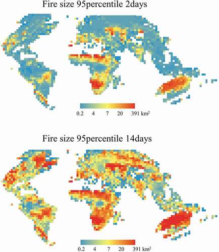
These approaches are problematic because the number and size of fires identified using such approaches are directly linked to the value of τ, and inappropriate selection of the value can severely impact the results. The sensitivity of the standard flood-fill algorithm to changes in τ is demonstrated in Figure 1. when applied to the MCD64A1 burned area product. Although the sensitivity to changes in τ is small within similar climatological zones, the differences between zones are more pronounced. For example, increasing τ from 2 days to 14 days results in large increases in apparent fire size in both Eastern Canada and the Brazilian Cerrado. In areas more prone to large, isolated fires like Eastern Canada, the 14-day temporal parameter yields reasonable results, while the same value is likely to result in over-aggregation within regions with high burning frequencies like the Cerrado. This observation corroborates the warning of Hantson et al. (2015) that the 14-day threshold ‘[…] could also result in an artificial increase in large fires for areas with a high burned fraction, which increases the chance that neighboring burn scars touch and are counted as one’. The variability in the result of flood-fill algorithm to the temporal threshold underscores the need to define the local variations in the speed at which fire spreads, even at coarse spatial resolutions. This, in turn, influences downstream analyses conducted on the individual fire level and enable better characterisation of fire behavior (e.g. Artés et al. 2019; Andela et al. 2019), emissions (Yue et al. 2014), and fire impact (Lasslop et al. 2019).

Figure 1. 95th percentile fire size calculated with temporal parameters of 2-days and 14-days using the standard flood-fill algorithm implementation. Note that fire size increases monotonically as the temporal parameter representing the threshold of cell-to-cell spread (in days) also increases.

In this work, we provide a method for defining an optimally-tuned Coarse-Resolution Rate of Spread (CRoS), ρ, for large regions according to the biome and vegetation cover using satellite detections of active fires. The resulting estimates of ρ, reported in km day⁻¹, at coarse spatial resolutions (250-m and coarser) can be used to make regional, empirically-driven adjustments to flood-fill algorithms, even with the comparatively low spatial precision of the measurements. These estimates can then be used as an input to inform the temporal parameter used by flood-fill algorithms at the pixel-level by recasting ρ into the time domain as $\tau =\delta /\rho$, where $\delta$ represents the (center-to-center) distance between a cell of a classified image and its neighbor (Figure 2). This work will therefore help reduce errors from over- and under-aggregation of individual fires by increasing the sensitivity of downstream fire extraction algorithms to differences in RoS based on satellite observations.

Figure 2. Proposed application of CRoS metric to burn patch extraction. (a) all available MCD14ML active fire locations are used as input to the (b) DBSCAN clustering and (c) fire spread tracking phases (see Figure 3 for additional details). (d) summary metrics, e.g., median CRoS (?), are calculate for each combination of Biomes-per-Realms and tree-cover category and converted into e) spatially explicit cell-to-cell ?-thresholds used to control f) flood-fill algorithms for individual burn patch extraction.

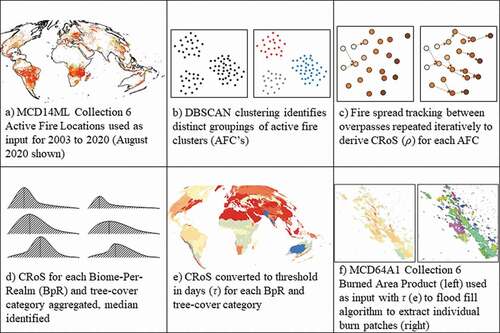
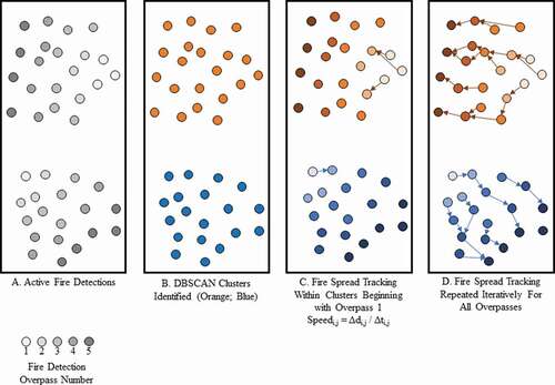
Figure 3. Illustration of the DBSCAN clustering and fire tracking approaches, with successive algorithm steps shown from left to right. Panel A shows two patches of MODIS fire pixels prior to clustering and tracking. Two fire clusters (orange and blue) are identified in panel B. MCD14ML detections from the first overpass are identified in each cluster in panel C the spread is “tracked,” assuming spread to the spread to the nearest (spatiotemporal) neighbour in subsequent overpasses. The spread tracking is repeated iteratively until no more neighbours are found within the spatiotemporal search radius.

2. Data

2.1. MODIS active fire data

The MODIS Collection 6 MCD14 ML (Giglio, Schroeder and Justice 2016) monthly active fire location product¹ provides a record of the daytime and nighttime detections from the Aqua and Terra platforms, including the location and time of detection of each active fire identified. The products are known to have a low rate of commission errors of 5% or less globally, except in Equatorial Asia, where the commission error rate was shown to be approximately 8% (Schroeder et al. 2008; Giglio, Schroeder and Justice 2016); thus, fires that are detected by the product can be used confidently. The detection algorithm primarily exploits electromagnetic radiation emitted in the middle-infrared portion of the spectrum, which is largely unaffected by the presence of smoke. However, there are instances in which thick clouds obscure active fires, which cannot be accounted for.

Though the product’s nominal cell size (at nadir) is 1 km, the algorithm is sensitive at the sub-pixel level and can detect flaming fires as small as ~50 m² in size under ideal conditions (Giglio et al. 2003). The active fire locations must consequently be considered approximate since the spatial quantisation of the pixel necessarily results in a loss of spatial precision. Both daytime and nighttime observations were used in the analysis. Only observations where the scan angle was within ±46.7° were used, corresponding to a maximum along-scan pixel dimension of 2 km. This restriction was used to limit the negative impacts of random artifacts stemming from the MODIS bowtie effect and pixel-center assignment of active fire locations. Importantly, active fire observations have lower temporal uncertainties than burned area products, enabling the calculation of ρ with higher accuracy than would be achievable using burned area products (Chuvieco et al. 2018; Boschetti et al. 2019; Humber et al. 2019).

2.2. Reference fire boundaries

Independently derived fire boundaries were used to identify the set of active fire locations belonging to the same event to facilitate the calculation of the CRoS. The importance of fire boundaries is magnified when using coarse satellite observations, where multiple distinct fires might occur in the same sensor sample. Unfortunately, official data about individual fires are not available in most countries. Eight sources of reference data covering nine countries were identified as useful for evaluating the results of this work (Table 2.).

Table 2. Fire boundary data from external sources

Official Name	Country	Region	Agency	Years	Citation
MTBS (fire perimeters)	US	Conterminous United States	MTBS	1984–2017	Picotte et al. (2020)
ABoVE (Wildfire Date of Burning within Fire Scars)	US, Canada	Alaska and Canada	NASA (ORNL DAAC)	2001–2015	Loboda and Hall (2017
BRazilian Fire-Land-Atmosphere System (BrFLAS)	Brazil	Brazilian Cerrado	BrFLAS	2015	Rodrigues et al. (2019)
EFFIS	Greece, Portugal, Spain	Whole country	JRC	2000–2020	San-Miguel-Ayanz et al. (2012)
̶	Russia	Kolyma River Basin in northeastern Siberia	NASA (ORNL DAAC)	1969–2007	Berner et al. (2016)
Data SA (Last Bushfire and Prescribed Burn Boundaries)	Australia	National Parks and Wildlife South Australia (NPWSA) reserves	Government of South Australia Department for Environment and Water	1931–2020	Data.SA (2020)
NAFI – Northern Australian Fire Information	Australia	Australian rangelands, excluding western NSW	Landgate WA, Geoscience Australia	2000–2019	NAFI (2019)
̶	Chile	Whole country	Universidad Mayor	2016–2018	P. Oliva (personal comm.)

An examination of the data showed that most datasets include records that fall into one or more of the following categories: (i) multiple records of the same fire; (ii) incompletely mapped fires, i.e. the fire started before or ended after scene pairs used for photointerpretation; (iii) cloud-obscured or otherwise unmapped areas were IMPROPERLY identified; (iv) implausible aggregation of separate fires into a single record. Records falling into any of these categories were removed, as were fires smaller than 200 ha, consistent with previous studies (Benali et al. 2016). While we assume that the reference fires are correctly classified, not all reference datasets are well-distributed within their respective countries and cannot be considered fully representative of the area’s fire regime.

2.3. Yearly forest/mixed/non-forest cover definitions

Clusters of active fires, defined in the Methods section, were categorised into forested, mixed, and non-forested land cover types depending on the proportion (specified below) of active fires coincident with forested and non-forested pixels defined in the Global Forest Change (GFC) dataset (Hansen et al. 2013). Each active fire location was compared to the GFC classification maps and was labeled as a fire-in-forest if the cell that burned was labeled as either extant forest (as of 2020) or was still forest at the time of the fire, e.g. the fire was labeled fire-in-forest if the fire occurred in 2005 and forest cover loss occurred in 2005 or later. Fires and forest cover losses occurring in the same year were labeled as fire-in-forest, as we assume that the fire caused the loss of forest. The mismatch of spatial resolutions (1 km and 30 m for the MCD14 ML and GFC datasets, respectively) was resolved by aggregating the GFC dataset to the 1-km MODIS resolution to generate annual binary forest/non-forest classifications where a cell received a ‘forest’ label if the simple majority of the contributing cells were identified as forest for a given year.

Fire clusters were extracted and categorised based on the percentage of the active fire locations labeled as fire-in-forest as follows: clusters with 90% or more of active fire locations located in forests were labeled as forest fires; clusters with between 10% and 90% of active fire locations located in forests were labeled as mixed fires; clusters with 10% or less of active fire locations located in forests were labeled as non-forest fires. While there are several definitions of the per cent tree cover that constitutes forest and non-forest, we elected to use these stricter thresholds to create more ‘pure’ classes.

2.4. Yearly cropland mask

Mapping fire activity in agricultural areas remains a known challenge (Hall et al. 2016; Boschetti et al. 2019). Specifically, in the context of this work, cropland burning can cause spurious results due to the proximity of many independent fires to one another, i.e. several agricultural fires can appear as single wildfire at coarse spatial resolutions. We used the Landcover CCI (ESA 2017) product to create yearly crop masks by aggregating the cropland and cropland-natural vegetation mosaic classes. Fire clusters with more than 10% of the active fire locations in cropland were discarded. The threshold was applied for each year in the study period, and the years that postdate the Landcover CCI product were assigned the value for 2018.

2.5. Biomes

Prior works stratified fire patterns at the ecoregion level by forest/non-forest covers (Abatzoglou et al. 2018; Zubkova et al. 2019). We similarly used the Ecoregions 2017 dataset (Dinerstein et al. 2017) to apply the forest/mixed/non-forest stratification at the biome level². Biomes were further separated by realms that approximately represent continents to distinguish between the same biome present in multiple continents (Figure S1).

3. Methods

3.1. Pixel-scale rate of spread calculation

We aimed to reconstruct the propagation of individual fires using MCD14 ML fire locations, ultimately generating a large sample of pixel-scale fire spread observations distributed globally. Our approach is based on the Fire Spread Reconstruction (FSR) method described by Loboda and Csiszar (2007). The FSR method uses the time series of active fire detections to track the likely path of a fire boundary across the land surface through time within a specific active fire cluster (AFC). The most likely path is reconstructed by identifying the nearest neighbor within spatial and temporal search radii, beginning with the overpass of the first active fire detection and proceeding iteratively through each subsequent overpass. The pixel-scale speed of the fire between satellite observations is then calculated based on the displacement between the locations of the active fire detections and the time between the overpasses. In the original implementation, thresholds of 2.5 km and 4 days were used as the spatial and temporal search radii, respectively. Despite its obvious shortcomings, the nearest neighbor assumption was adopted in the original algorithm implementation as a ‘reasonable assumption of fire behavior’ by the authors (Loboda and Csiszar 2007).

FSR has two components: (i) identification of active fire clusters and (ii) calculation of the pixel-scale CRoS (ρ). The first component of the FSR approach – identification of AFCs – is arguably too computationally intensive to apply globally using the Loboda and Csiszar (2007) method and benefits from a priori knowledge of specific AFCs. Unfortunately, as documented in other works (Boschetti et al. 2019), high-quality reference datasets that capture fire activity over large areas are rare. Therefore, we used a data mining approach to identify AFCs representing distinct fire events from 2001 to 2019. AFCs consist of multiple active fire detections (i.e. including the location and time) corresponding to one distinct fire. These clusters were selected from a database of all MCD14 ML records using the density-based spatial clustering of applications with noise (DBSCAN) clustering algorithm (Ester et al. 1996) implemented in the Python Scikit-Learn library (Pedregosa et al. 2011). DBSCAN is a commonly used density-based clustering algorithm that identifies clusters of points by searching for core points and establishing their connectivity to non-core points based on distance. A point is determined to be a core point if it has more than the minimum number of neighbors within a specified search radius. Points located within the search radius of the core point are added to the cluster, and the process is repeated iteratively until all points are either assigned to a cluster or are determined to be noise if the point is not a member of a cluster.

DBSCAN therefore requires two parameters: a neighborhood radius and a minimum cluster core size required to identify a cluster’s core points. The neighborhood radius parameter (ε) was set to 8050, based on the ‘worst-case’ parameters for the FSR spread rate calculation (i.e. the 3-dimensional Euclidean distance of the spatial search radius of 2,500 m and temporal window of 7,200 minutes, or 5 days). The FSR approach’s original thresholds informed the neighborhood radius parameter, i.e. 2.5 km and 4 days. However, we increased the temporal threshold to 5 days because the original FSR algorithm was implemented for Russia, which receives more satellite overpasses than lower-latitude regions of the world. The minimum cluster core size parameter – a threshold for the minimum number of active fire locations within the neighborhood radius required to form a cluster core – was set to 25 active fire locations. Increasing the minimum core size or decreasing the neighborhood radius favors the selection of larger fires, while decreasing the core size or increasing the search radius leads to over-aggregation of independent fires or inclusion of fires with too few data points to be representative of the CRoS. MCD14 ML locations and observation times were used as input to the DBSCAN algorithm, with the location coordinates transformed from the geographic coordinate system to the world equidistant cylindrical projection to reduce distance distortions.

The AFCs were used as input into the second component of the FSR approach to calculate the CRoS. Based on the approach outlined by Loboda and Csiszar (2007), the active fire locations within each AFC were analyzed iteratively to determine the most likely fire spread path, using the original 2.5 km spatial search radius but increasing the spatial search radius from 4 days to 5 days. The CRoS of each active fire location with a qualified nearest neighbor (within the spatial and temporal search radii) was calculated as the distance between the fire locations divided by the difference between the fire locations’ observation times. The calculated speed is omnidirectional, as it does not specify movement in a heading, flanking, or backing direction (Figure 3). A minimum threshold of 30 minutes between overpasses was implemented to reduce artifacts from Aqua and Terra overpasses at near coincident times. Such artifacts result in implausibly high speeds due to the random placement of the actual fire location within a ground sample, further exacerbated by the bowtie effect, that can make an active fire location appear to move a significant distance over a short period, resulting in high fire speed attributable to (random) view angle effects. The geodesic distance was calculated by applying the haversine transformation to the fire latitude/longitude coordinates rather than using a projected coordinate system with significant distance distortions at high latitudes.

The CRoS for each cluster was defined by the median and 95^th percentile speed for all pairs within a specific AFC. Each AFC was further associated with a biome, realm, and forest/mixed/non-forest label based on the mode of the active fire locations. The 95^th percentile was chosen as an indicator of the maximum fire speed observed that is more robust to outliers and processing artifacts than the maximum itself. The calculation accounts for only the scalar speed and should not be confused with the rate of forward spread. AFCs were discarded if the fire duration was less than 48 hours to reduce the contribution of noisy clusters.

At this point, it is necessary to disambiguate the CRoS derived from polar-orbiting observations calculated in this study from field observations. Specifically, field observations of the fire’s rate of spread pertain to the forward rate of fire spread during its most active period, over shorter time intervals, and with highly precise spatial and temporal measurements. In contrast, the active fire data derived from polar-orbiting sensors in this work are far less precise. Each MODIS sensor orbits the Earth approximately once per 90 minutes and can take two days to image a specific location on the surface, assuming clear-sky conditions. Furthermore, the uncertainty of the location of the fire within the cell is a function of the scan angle, the temperature of the fire, and the size of the fire. At nadir viewing geometry, the uncertainty is limited to approximately 500-m, or half of the width of a 1-km cell, with the maximum uncertainty increasing as the scan angle increases. Satellite-based measurements therefore have an inherently higher spatial uncertainty and are integrated over longer time intervals compared to field-based measurements.

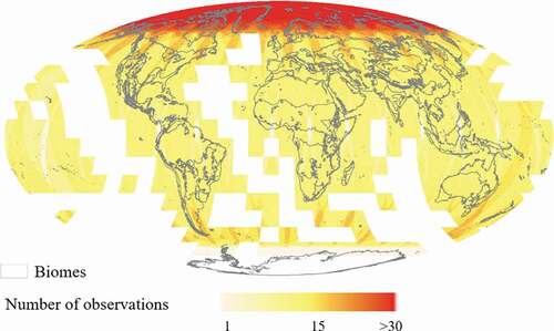
Consequently, there are two key distinctions between the spread rate metrics based on field observations and the metrics from the present method. First, the method described in this work does not specify the direction of the fire, i.e. it is not the forward rate of spread; rather, it is the overall spread rate in the heading, flanking, and backing directions. Second, the number of observations is constrained by the polar-orbiting nature of the satellites themselves, as illustrated in Figure 4. The number of times a location is imaged over a set period varies with latitude (and, as a corollary, so does time between observations). The worst-case scenario occurs at the Equator, where some locations will only be observed twice per day (morning and night overpasses), resulting in a mean re-imaging time of 12 hours. On the other hand, a location near the poles can be observed several dozen times per day, resulting in a mean re-imaging time of less than one hour. Because fires do not sustain their activity peaks over long periods (as a result of diurnal cycles at the macro-scale and variability of moisture, fuel loads, topography, and other factors at micro-scales), this method is more likely to observe the actual peak of the fire activity at high latitudes than near the Equator due to the shorter time between observations and the higher number of observations.

Figure 4. Number of MODIS observations (Aqua and Terra) on 1 July 2020, derived from the MOD09GA and MYD09GA products. White indicates regions with no observations.

3.2. Framework for accuracy assessment

Reference boundaries of known fires, determined by official or semi-official agencies (Table 2), were used to identify active fire locations belonging to the same fire event, analogous to the AFCs identified in the previous steps. Each combination of fire boundaries and active fire locations was visually inspected to ensure that the number of active fire detections was adequate to characterise the fire and that the boundary itself was of good quality. Active fire locations were considered to belong to the official/semi-official fire boundary if they overlapped the extent of the fire boundary and were detected on or between the start and end dates of the fire event, as reported by the agency. The set of active fire locations meeting these criteria forms the reference AFC.

The AFCs extracted using DBSCAN were compared to the reference AFC with the most common active fire locations. The success of the DBSCAN method was determined by the proportion of correctly selected active fire locations, i.e. the number of correctly identified fire locations relative to the set of unique fire locations in both the reference and extracted AFCs. To quantify the effects of the DBSCAN clustering accuracy on the CRoS, the CRoS of the extracted AFCs were compared to the CRoS of active fires overlapping the reference AFC dataset using the same FSR approach. The accuracy is reported using two metrics: the per cent of correctly identified active fire locations in an AFC and the active fire locations in the corresponding reference fire, and the CRoS calculated for corresponding AFC and reference data pairs.

4. Results

4.1. Global pixel-scale fire spread rates

The DBSCAN clustering operation identified a total of 168,777 AFCs from approximately 90 million MCD14 ML fire detections. The pixel-scale fire spread rates derived in this work are presented in Figure 5 and Table 3. For comparison with other works, the 95^th percentile CRoS, which more closely approximates the maximum fire spread rate, was calculated in addition to the median CRoS of each biome per realm (BpR).

Figure 5. Median CRoS in areas with fire activity (>0.005 active fires km-1 yr-1) masked by (a) forest (>=90% tree cover), (b) mixed (tree cover >10% and <90%), and non-forested (<=10% tree cover) land covers. Only ecoregions with >0.05% mean annual burned area are shown, determined using the MCD64A1 Collection 6 Burned Area Product (Giglio et al. 2018).

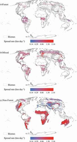
Table 3. CRoS (ρ; km day^-1) per biome disaggregated by forested (≥90% tree cover), mixed (10≥% tree cover <90), and non-forested (<10% tree cover) land covers. Agricultural fires excluded (>10% fires in agricultural land covers). Biomes with <30 fire clusters excluded

Realm	Biome	Forest		Mixed		Non-Forest
		Median	95^th	Median	95^th	Median	95^th
Afrotropic	Deserts & Xeric Shrublands	-	-	0.29	2.39	1.94	15.09
Afrotropic	Flooded Grasslands & Savannas	1.18	7.91	0.59	14.01	1.69	18.17
Afrotropic	Mangroves	-	-	0.06	6.11	0.10	5.72
Afrotropic	Mediterranean Forests, Woodlands & Scrub	0.88	3.34	1.14	10.47	1.25	10.25
Afrotropic	Montane Grasslands & Shrublands	-	-	0.86	10.41	0.61	14.01
Afrotropic	Tropical & Subtropical Dry Broadleaf Forests	0.58	15.74	0.59	9.71	0.62	13.15
Afrotropic	Tropical & Subtropical Grasslands, Savannas & Shrublands	0.73	15.98	0.76	16.59	1.30	17.67
Afrotropic	Tropical & Subtropical Moist Broadleaf Forests	0.68	13.77	0.61	14.67	0.91	16.04
Australasia	Deserts & Xeric Shrublands	1.43	4.72	1.43	7.13	1.61	13.57
Australasia	Mediterranean Forests, Woodlands & Scrub	0.95	7.07	0.85	11.48	0.78	10.24
Australasia	Temperate Broadleaf & Mixed Forests	0.71	9.66	0.75	8.41	0.32	4.28
Australasia	Temperate Grasslands, Savannas & Shrublands	-	-	0.68	4.21	0.76	7.11
Australasia	Tropical & Subtropical Dry Broadleaf Forests	-	-	0.06	11.20	0.09	5.54
Australasia	Tropical & Subtropical Grasslands, Savannas & Shrublands	1.25	7.03	0.75	8.58	1.30	15.16
Australasia	Tropical & Subtropical Moist Broadleaf Forests	0.33	8.71	0.72	7.47	0.26	8.61
Indomalayan	Deserts & Xeric Shrublands	-	-	1.18	10.15	1.74	11.26
Indomalayan	Mangroves	0.32	8.52	0.39	9.56	-	-
Indomalayan	Temperate Broadleaf & Mixed Forests	0.40	2.16	0.43	3.86	-	-
Indomalayan	Tropical & Subtropical Coniferous Forests	0.99	4.65	0.98	5.08	-	-
Indomalayan	Tropical & Subtropical Dry Broadleaf Forests	0.35	4.82	0.49	14.44	0.65	14.67
Indomalayan	Tropical & Subtropical Grasslands, Savannas & Shrublands	0.85	4.74	0.84	3.21	-	-
Indomalayan	Tropical & Subtropical Moist Broadleaf Forests	0.61	7.68	0.59	9.09	0.09	11.02
Nearctic	Boreal Forests/Taiga	0.71	14.85	0.69	14.69	0.61	12.23
Nearctic	Deserts & Xeric Shrublands	-	-	0.82	13.33	0.36	17.70
Nearctic	Mediterranean Forests, Woodlands & Scrub	0.65	6.12	1.04	11.23	1.30	9.26
Nearctic	Temperate Broadleaf & Mixed Forests	0.79	16.85	0.94	13.93	0.10	5.13
Nearctic	Temperate Conifer Forests	0.45	9.81	0.49	11.35	1.07	16.79
Nearctic	Temperate Grasslands, Savannas & Shrublands	0.42	15.05	0.85	17.60	1.61	28.17
Nearctic	Tropical & Subtropical Coniferous Forests	0.58	3.44	0.72	5.57	0.99	7.34
Nearctic	Tundra	0.62	12.37	0.56	11.82	0.59	12.33
Neotropic	Deserts & Xeric Shrublands	-	-	0.19	11.15	0.07	6.26
Neotropic	Flooded Grasslands & Savannas	0.62	7.50	0.88	9.91	1.05	9.53
Neotropic	Mangroves	0.75	2.51	0.95	9.62	0.92	9.25
Neotropic	Mediterranean Forests, Woodlands & Scrub	-	-	0.94	6.39	0.65	3.33
Neotropic	Montane Grasslands & Shrublands	-	-	0.92	6.65	1.08	8.45
Neotropic	Temperate Broadleaf & Mixed Forests	0.55	3.96	0.68	10.89	0.07	4.54
Neotropic	Temperate Grasslands, Savannas & Shrublands	1.45	4.51	0.75	3.21	1.84	20.30
Neotropic	Tropical & Subtropical Coniferous Forests	0.59	10.17	0.79	8.86	0.65	9.49
Neotropic	Tropical & Subtropical Dry Broadleaf Forests	0.58	10.24	0.66	10.84	0.82	9.43
Neotropic	Tropical & Subtropical Grasslands, Savannas & Shrublands	0.62	9.55	1.02	13.97	1.63	16.78
Neotropic	Tropical & Subtropical Moist Broadleaf Forests	0.52	10.04	0.62	11.84	1.41	15.32
Oceania	Tropical & Subtropical Dry Broadleaf Forests	-	-	0.01	11.79	0.01	1.81
Oceania	Tropical & Subtropical Moist Broadleaf Forests	-	-	0.01	0.99	0.07	1.20
Palearctic	Boreal Forests/Taiga	0.58	11.19	0.56	13.39	0.26	15.52
Palearctic	Deserts & Xeric Shrublands	0.06	0.66	1.38	20.38	0.09	24.65
Palearctic	Flooded Grasslands & Savannas	1.25	15.67	2.82	28.02	0.09	25.07
Palearctic	Mediterranean Forests, Woodlands & Scrub	0.78	4.23	0.94	15.74	0.09	6.31
Palearctic	Montane Grasslands & Shrublands	-	-	0.69	13.77	0.17	15.15
Palearctic	Temperate Broadleaf & Mixed Forests	0.88	17.14	1.59	24.83	0.07	14.67
Palearctic	Temperate Conifer Forests	0.62	14.62	1.02	21.38	2.17	19.12
Palearctic	Temperate Grasslands, Savannas & Shrublands	0.66	13.26	1.14	21.21	0.85	28.05
Palearctic	Tropical & Subtropical Moist Broadleaf Forests	0.68	2.46	0.91	10.24	0.07	1.57
Palearctic	Tundra	0.56	10.09	0.58	12.79	0.16	13.42

In 22 out of 36 BpR with significant fire activity in forested and non-forested land, the 95^th percentile CRoS (used to approximate the maximum CRoS) in non-forested areas was greater than the 95^th percentile CRoS in forested areas. Similarly, 26 out of 36 BpR demonstrated the same pattern when considering the median CRoS. The fastest fires were found in the Palearctic and Nearctic realms’ Temperate Grasslands, Savannas & Shrublands biome (28.17 and 28.05 km day⁻¹ respectively), due to the spread of massive fires observed yearly in Russia’s Jewish Autonomous Oblast along the Amur River in the Palearctic realm and yearly prairie fires observed in the central United States in the Nearctic realm. CRoS in Palearctic Temperate Grasslands, Savannas & Shrublands were among the fastest observed in this study due to large fast-moving fires in the Kazakh Steppe, which were also annual occurrences. Slower fires (less than .2 km day⁻¹) were observed in BpR’s characterised by very low biomass (e.g. Deserts & Xeric Shrublands in the Neotropic and Palearctic realms) or high precipitation (e.g. Mangroves in Oceania). In the most fire-prone continents, Africa and Australia, the fastest fires, by median CRoS, were associated with high inter-annual variability in rainfall (Fatichi, Ivanov and Caporali 2012), e.g. Deserts & Xeric Shrublands.

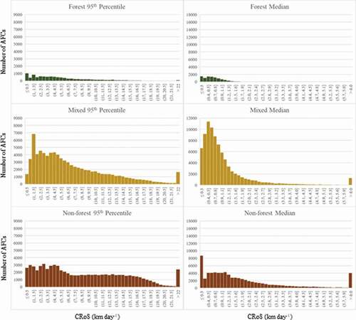
The distribution of pixel-scale fire spread rates is strongly right-skewed, favoring lower CRoS with few (but very fast-moving) outliers (Figure 6). In line with expectations, the CRoS tended to be highest for non-forest fires, followed by mixed forest/non-forest fires, while forest fires had the slowest CRoS, as indicated by the relative proportion of fires in higher CRoS bins from fastest to slowest.

Figure 6. Histogram of fire speeds in forested (top), mixed (middle), and non-forested (bottom) land covers.

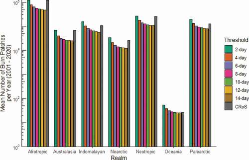
When adjusting for the distance between cells, these results show that, in most biomes, the cell-to-cell spread time, τ, for 500-meter MODIS cells is typically less than two days – well below many of the thresholds used previously (Table 1). Applying the τ thresholds, calculated from ρ values, to the burn patch extraction workflow (Figure 2) yields plausible results and, qualitatively, compares favorably to the Fire Atlas (Andela et al. 2019) in regions where fires overlap and merge throughout the year (Figure 7). To demonstrate the effects of different τ thresholds on burn patch extraction, the standard flood-fill algorithm described by Archibald and Roy (2009) was implemented for τ = {2, 4, 6, 8, 10, 12, 14} days, spanning the range of values used in other studies (e.g. Table 1). The number of burn patches identified within the range of values was compared to the same method implementing the CRoS, ρ (km day⁻¹), transformed into τ (days pixel⁻¹), calculated for each BpR in this study. The results were aggregated to realms, excluding Antarctica. Given that the flood-fill algorithm is a complete segmentation of the pixels classified as burned by the MCD64A1 product, the number of burn patches identified per year decreases monotonically as τ increases (Figure 8). In the Afrotropic, Australasian, and Neotropic realms, the CRoS-based method behaves most similarly to τ = 2 days, while the Indomalayan, Nearctic, and Palearctic realms are more similar to τ = 4 days. In Oceania, the CRoS behavior is most similar to τ = 12 days. Even at the coarser realm levels, these differences underline the importance of selecting appropriate τ for different spatial locations to provide realistic representations of individual burn patches that are sensitive to changes in the underlying drivers of fire spread.

Figure 7. Burn patch extraction examples for two scenes in 2015 from Kazakhstan (top row) and Australia (bottom row). Boxes (a) and (d) show the input MCD64A1 Collection 6 burned area product, boxes (b) and (e) show the Fire Atlas “perimeters” dataset for comparison, and boxes (c) and (f) illustrate the result of burn patch identification using the proposed CRoS threshold approach. For the Fire Atlas and CRoS-derived patches, each unique colour represents a distinct burn patch.

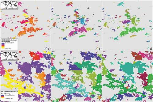
Figure 8. Mean number of burn patches identified per year for a range of threshold values (?) between 2001 and 2020. The CRoS-based parameter is implemented at the BpR unit for the forest/mixed/non-forest cover types and adjusted for displacement of the sinusoidal projection using the haversine transformation, with results aggregated to the realm unit.

4.2. Clustering accuracy assessment

The correspondence between AFCs extracted using the DBSCAN method and the reference dataset is depicted in Figure 9. Comparison to the independent reference data shows that the performance of the DBSCAN clustering method is best in the datasets covering North America, Australia, and Siberia. In contrast, the performance is more variable and less accurate in Portugal, Chile, Spain, and Brazil. The best performance is found in areas where the reference dataset was characterised by either large or isolated fires, while areas with smaller reference fires do not perform as well. Therefore, spatial resolution may be a limiting factor in the clustering operation.

Figure 9. Box plots of the percent of active fire locations correctly identified by AFCs compared to reference datasets. The sample size for each dataset can be found in Table 3.

The impact of errors in AFC identification on the CRoS is generally low, with a mean error of less than ±.09 km day⁻¹ except in Canada and Alaska, where the mean error was −.96 km day⁻¹ (Table 4). The impact of random errors at high latitudes (discussed in the Methods section) is a likely driver of the higher errors in Canada and Alaska. The Normalised RMSE (NRMSE) indicates that errors in the spread rate were less than 10% for all reference datasets except Portugal and Chile. The CRoS error and the number of fire locations identified in the cluster were weakly correlated in all cases, indicating that the number of samples does not bias the CRoS.

Table 4. Accuracy assessment of the rate of spread from the DBSCAN clustering method and reference fire boundaries

Location	# Fires	Mean Error (km day^−1)	RMSE (km day^−1)	NRMSE (%)	Error-Size Correlation (r)
All	2229	−.06	0.39	2.58	−.12
Australia (Data SA)	225	−.04	0.23	6.96	0.00
Australia (NAFI)	520	−.03	0.23	3.52	−.08
Brazil	44	−.11	0.46	8.59	−.19
Canada, AK (ABoVE)	542	−.96	0.25	3.00	−.14
Chile	29	0.04	0.24	18.68	−.04
CONUS (MTBS)	583	−.05	0.54	5.97	−.03
Greece	35	0.01	0.36	7.19	0.14
Portugal	131	−.09	0.70	13.36	−.02
Siberia	23	−.01	0.20	8.79	0.02
Spain	96	0.03	0.48	6.77	0.04

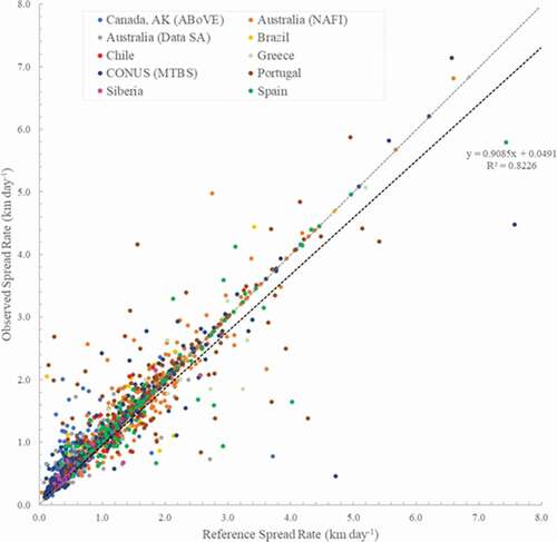
The relationship between the CRoS of AFCs and reference fires is shown in Figure 10. The overall agreement between reference and observed values is high (R² = .82), though the fastest-moving fires’ speed tends to be somewhat underestimated using the DBSCAN clustering method, resulting in an overall slope of .91.

Figure 10. Scatterplot of the median spread rate of individual fires for reference and observed AFCs.

5. Discussion and conclusions

In this work, we estimated pixel-scale fire CRoS for different biomes in forested, mixed, and non-forested land covers. This variable is suitable for improving fire patch extraction algorithms using coarse resolution burned area products. Individual fire events were defined by extracting AFCs by mining the entire MCD14 ML archive using the DBSCAN clustering algorithm. The CRoS was calculated using the FSR approach (Loboda and Csiszar 2007) applied to each AFC. The median and 95^th percentile CRoS’s were presented for each terrestrial biome with fire activity, and the accuracy of the CRoS was evaluated by comparison to active fires within independently derived reference fire boundaries.

CRoS values calculated in this work generally agree with other published works (McCaw et al. 2012; Dupire et al. 2019; Gould and Sullivan 2020), and these results replicate the original algorithm implementation in Russia by Loboda and Csiszar (2007). Cruz et al. (2018) reviewed CRoS ranges from field observations of wildfires and prescribed fires, compiling a comprehensive list of previously published studies in different biomes/realms, which vary from .1–20 m min⁻¹ (~.15–28.8 km day⁻¹) in forests to .2–160 m min⁻¹ (~.3–230.4 km day⁻¹) in grassland. However, comparisons of spread rates observed using our method and those obtained by field observation should be viewed critically because the measurements are made at fundamentally different spatial and temporal scales with large differences in the instruments’ precision. Key differences between the two types of observations include: field studies may seek out powerful and faster-moving fires (McCaw et al. 2012); field studies may observe fires over smaller distances and shorter time intervals than can be detected by MCD14 ML (Cruz et al. 2010; Johnston et al. 2018; N’Dri et al. 2018); other studies measure fires during the peak of the fire season and in the middle of the day when fires are most intense (Sullivan 2010; McCaw et al. 2012) while our study also includes fire spread overnight and outside of the main burning season (Matthews et al. 2012); and, as in the original algorithm implementation, we assume active fires spread to their nearest neighbor in subsequent satellite overpasses – while we agree this is a reasonable assumption, it is an omnidirectional measure of the fire spread that necessarily results in fire spread covering the shortest possible distance over time and will therefore tend to underestimate the true speed of the fire spread.

In light of these findings, we also acknowledge some potential future improvements that could be made to this method. One such improvement would be to normalise the time and space dimensions of the active fire observations to prevent over-weighting the time dimension in the DBSCAN search radius parameter. While it is unlikely that the non-normalisation of the input data biased the results because of the CRoS calculation restrictions, more clusters could likely have been detected overall using a more well-balanced time-space threshold. Additionally, an unknown level of error can be attributed to the MODIS sensor’s coarse spatial resolution. As the length of the newer Visible Infrared Imaging Radiometer Suite (VIIRS) archive increases and the associated active fire products mature, the finer 375-m spatial resolution of the VIIRS instrument would likely improve these results. Unfortunately, any such improvements would have to be balanced against the loss of the Terra-like morning overpass.

Similarly, there is evidence that the performance of the GFC dataset used to stratify the forest/mixed/non-forest land cover types may vary depending on the type of tree cover loss (harvest or fire) in some regions (Guindon et al. 2018). It is, therefore, possible that the CRoS calculated in this work may propagate underestimation errors related to forest regrowth in the GFC product, causing forest fires to be included in the mixed or non-forest classes.

A limitation of this work stems from the use of polar-orbiting satellite observations. The CRoS calculated near the poles will more closely replicate field observations taken at the fire activity peak because the time between images is short, and there are more observations in total. In contrast, the values calculated near the Equator, with more time between observations, will average short periods of high fire activity with long periods of low fire activity, likely biasing the CRoS toward the low end of observed values. Geostationary observations could solve this problem, but no reliable, harmonised product with global coverage exists at the time of this work.

The method presented in this work uses a subset of the total available data, derived by discarding active fire detections for which satellite overpasses were temporally close or where the sensor scan angle was unfavorable to reduce the effects of the random locations of fires within the sensor’s instantaneous field of view (IFOV). Such concessions are necessary because, in a worst-case scenario, the same fire may be observed by near-coincident satellite overpasses at far off-nadir viewing geometry. In such a scenario, the actual displacement of the fire between observations would be near-zero, and the time between observations would also be near-zero. However, random effects can lead to an observed displacement of several kilometers; thus the numerator of the rate, consisting almost entirely of noise, leads to high calculated CRoS while the actual CRoS is close to zero. In effect, removing such data points leads to metrics calculated over larger distances where the signal (distance between active fires) is much greater than the noise (random location of actual active fires within the IFOV). This theoretically reduces the sensitivity of our approach over short timeframes, but in practice, this is outweighed by the reduction of implausibly high CRoS values based on observation noise.

This work also relies on the selection of two free parameters, the neighborhood radius parameter (ε) and the minimum cluster core size. The thresholds used in this work (8050 and 25, respectively) were selected based on visual inspection of many different thresholds. In extreme cases, smaller minimum cluster core sizes and/or larger radius parameters caused all fire activity in areas with high fire activity (e.g. Africa and Australia) to be selected into a single fire event each fire season. On the other hand, larger minimum cluster core sizes and/or smaller radius parameters resulted in significant increases in the number of fires excluded from the dataset in the mid-latitudes, where the number of daily satellite overpasses and fire activity are lower.

Ultimately, the goal of this work was to provide a global baseline estimate of the CRoS of wildfires at coarse spatial resolution (pixel scale) to improve the delineation of individual fires from global burned area products with flood-fill-based algorithms. Our finding that the value of τ, derived from coarse resolution observations, is less than two days for many regions suggests that flood-fill fire extraction algorithms that apply a uniform temporal parameter are likely using values that are too large in most of the world, which can lead to over-aggregation of distinct burns into one fire. The CRoS values in this paper can provide a basis for modifying the parameter regionally and based on land cover type. The active fire product used in this study can be considered independent of the burned area products used for burn patch extraction in downstream workflows. Consequentially, these results can be used to improve the accuracy of fire extraction algorithms by providing location-adjusted estimates of cell-to-cell fire spread based on historical observations.

Acknowledgments

This work was funded by NASA grants 80NSSC18K0739 and 80NSSC18K0619. We thank Dr. Patricia Oliva (Universidad Mayor, Chile) for providing Chilean fire boundaries data (Project name: ‘Using Sentinel-2 images to develop an automatic burned area mapping algorithm’, Project Reference: FONDECYT Iniciación #11181331).

Supplementary material

Supplemental data for this article can be accessed here.

Disclosure statement

No potential conflict of interest was reported by the author(s).

Data availability statement

The data that support the findings of this study are available from the corresponding author, M.H., upon reasonable request.

Additional information

Funding

The work was supported by the Goddard Space Flight Center [80NSSC18K0619,80NSSC18K0739]

References

- Abatzoglou, J. T., A. P. Williams, L. Boschetti, M. Zubkova, and C. A. Kolden. 2018. “Global Patterns of Interannual Climate–fire Relationships.” Global Change Biology 24 (11): 5164. doi:https://doi.org/10.1111/gcb.14405.
- Albini, F. A. 1985. “A Model for Fire Spread in Wildland Fuels.” Combustion Science and Technology 42 (5–6): 229. doi:https://doi.org/10.1080/00102208508960381.
- Alexander, M. E. and M. G. Cruz. 2013. “Limitations on the Accuracy of Model Predictions of Wildland Fire Behaviour: A State-of-the-Knowledge Overview.” The Forestry Chronicle 89 (3): 372. doi:https://doi.org/10.5558/tfc2013-067.
- Alexandridis, A., D. Vakalis, C. I. Siettos, and G. V. Bafas. 2008. “A Cellular Automata Model for Forest Fire Spread Prediction: The Case of the Wildfire That Swept Through Spetses Island in 1990.” Applied Mathematics and Computation 204 (1): 191. doi:https://doi.org/10.1016/j.amc.2008.06.046.
- Andela, N., D. C. Morton, L. Giglio, R. Paugam, Y. Chen, S. Hantson, G. R. van der Werf, and J. T. Randerson. 2019. “The Global Fire Atlas of Individual Fire Size, Duration, Speed and Direction.” Earth System Science Data 11 (2): 529. doi:https://doi.org/10.5194/essd-11-529-2019.
- Andela, N., D. C. Morton, L. Giglio, Y. Chen, G. R. van der Werf, P. S. Kasibhatla, R. S. DeFries et al. 2017. ”A Human-Driven Decline in Global Burned Area.” Science 356 (6345): 1356. doi:https://doi.org/10.1126/science.aal4108.
- Archibald, S., C. E. R. Lehmann, J. L. Gomez-Dans, and R. A. Bradstock. 2013. “Defining Pyromes and Global Syndromes of Fire Regimes.” Proceedings of the National Academy of Sciences 110 (16): 6442. doi:https://doi.org/10.1073/pnas.1211466110.
- Archibald, S. and D. P. Roy. 2009. “Identifying Individual Fires from Satellite-Derived Burned Area Data.” In International Geoscience and Remote Sensing Symposium (IGARSS), Vol. 3. doi:https://doi.org/10.1109/IGARSS.2009.5417974.
- Artés, T., D. Oom, D. de Rigo, T. H. Durrant, P. Maianti, G. Libertà, and J. San-Miguel-Ayanz. 2019. “A Global Wildfire Dataset for the Analysis of Fire Regimes and Fire Behaviour.” Scientific Data 6 (1): 296. doi:https://doi.org/10.1038/s41597-019-0312-2.
- Benali, A., A. Russo, A. C. L. Sá, R. M. S. Pinto, O. Price, N. Koutsias, and J. M. C. Pereira. 2016. “Determining Fire Dates and Locating Ignition Points with Satellite Data.” Remote Sensing 8 (4): 326. doi:https://doi.org/10.3390/rs8040326.
- Berner, L. T., P. S. A. Beck, M. M. Loranty, H. D. Alexander, M. C. Mack, and S. J. Goetz. 2016. ”Siberian Boreal Forest Aboveground Biomass and Fire Scar Maps, Russia, 1969-2007.” Ornl Daac, doi:https://doi.org/10.3334/ORNLDAAC/1321.
- Boschetti, L., D. P. Roy, L. Giglio, H. Huang, M. Zubkova, and M. L. Humber. 2019. “Global Validation of the Collection 6 MODIS Burned Area Product.” Remote Sensing of Environment 235 (December): 111490. doi:https://doi.org/10.1016/j.rse.2019.111490.
- Chuvieco, E., J. Lizundia-Loiola, M. L. Pettinari, R. Ramo, M. Padilla, K. Tansey, F. Mouillot et al. 2018. ”Generation and Analysis of a New Global Burned Area Product Based on MODIS 250-M Reflectance Bands and Thermal Anomalies.” Earth System Science Data 10 (4): 2015. doi:https://doi.org/10.5194/essd-10-2015-2018.
- Cruz, M. G., J. S. Gould, M. E. Alexander, A. L. Sullivan, W. L. McCaw, and S. Matthews. 2015. “Empirical-Based Models for Predicting Head-Fire Rate of Spread in Australian Fuel Types.” Australian Forestry 78 (3): 118. doi:https://doi.org/10.1080/00049158.2015.1055063.
- Cruz, M. G., M. E. Alexander, A. L. Sullivan, J. S. Gould, and M. Kilinc. 2018. “Assessing Improvements in Models Used to Operationally Predict Wildland Fire Rate of Spread.” Environmental Modelling & Software 105 (July): 54. doi:https://doi.org/10.1016/j.envsoft.2018.03.027.
- Cruz, M. G., M. E. Alexander, and R. H. Wakimoto. 2005. “Development and Testing of Models for Predicting Crown Fire Rate of Spread in Conifer Forest Stands.” Canadian Journal of Forest Research 35 (7): 1626. doi:https://doi.org/10.1139/x05-085.
- Cruz, M. G., S. Matthews, J. Gould, P. Ellis, M. Henderson, I. Knight, and J. Watters. 2010. “Fire Dynamics in Mallee-Heath: Fuel, Weather and Fire Behaviour Prediction in South Australian Semi-Arid Shrublands.” Bushfire Cooperative Research Centre, Report A 10 1–140 .
- Data.SA. 2020. Last Bushfire and Prescribed Burn Boundaries. Government of South Australia. https://data.sa.gov.au/data/dataset/last-fire.
- Dinerstein, E., D. Olson, A. Joshi, C. Vynne, N. D. Burgess, E. Wikramanayake, N. Hahn et al. 2017. ”An Ecoregion-Based Approach to Protecting Half the Terrestrial Realm.” BioScience 67 (6): 534. doi:https://doi.org/10.1093/biosci/bix014.
- Duff, T. J., D. M. Chong, and K. G. Tolhurst. 2013. “Quantifying Spatio-Temporal Differences Between Fire Shapes: Estimating Fire Travel Paths for the Improvement of Dynamic Spread Models.” Environmental Modelling & Software 46 (August): 33. doi:https://doi.org/10.1016/j.envsoft.2013.02.005.
- Dupire, S., T. Curt, S. Bigot, and T. Fréjaville. 2019. “Vulnerability of Forest Ecosystems to Fire in the French Alps.” European Journal of Forest Research 138 (5): 813. doi:https://doi.org/10.1007/s10342-019-01206-1.
- ESA. 2017. “Land Cover CCI Product User Guide Version 2.” Tech. Rep. http://maps.elie.ucl.ac.be/CCI/viewer/download/ESACCI-LC-Ph2-PUGv2_2.0.pdf
- Ester, M., H.-P. Kriegel, J. Sander, and X. Xu. 1996. “A Density-Based Algorithm for Discovering Clusters in Large Spatial Databases with Noise.” Kdd 96: 226.
- Fatichi, S., V. Y. Ivanov, and E. Caporali. 2012. “Investigating Interannual Variability of Precipitation at the Global Scale: Is There a Connection with Seasonality?” Journal of Climate 25 (16): 5512. doi:https://doi.org/10.1175/JCLI-D-11-00356.1.
- Giglio, L., J. Descloitres, C. O. Justice, and Y. J. Kaufman. 2003. “An Enhanced Contextual Fire Detection Algorithm for MODIS.” Remote Sensing of Environment 87 (2): 273. doi:https://doi.org/10.1016/S0034-4257(03)00184-6.
- Giglio, L., L. Boschetti, D. P. Roy, M. L. Humber, and C. O. Justice. 2018. “The Collection 6 MODIS Burned Area Mapping Algorithm and Product.” Remote Sensing of Environment 217: 72. doi:https://doi.org/10.1016/j.rse.2018.08.005.
- Giglio, L., W. Schroeder, and C. O. Justice. 2016. “The Collection 6 MODIS Active Fire Detection Algorithm and Fire Products.” Remote Sensing of Environment 178 (June): 31. doi:https://doi.org/10.1016/j.rse.2016.02.054.
- Gould, J. S. and A. L. Sullivan. 2020. “Two Methods for Calculating Wildland Fire Rate of Forward Spread.” International Journal of Wildland Fire 29 (3): 272. doi:https://doi.org/10.1071/WF19120.
- Guindon, L., P. Bernier, S. Gauthier, G. Stinson, P. Villemaire, and A. Beaudoin. 2018. “Missing Forest Cover Gains in Boreal Forests Explained.” Ecosphere 9 (1): e02094. doi:https://doi.org/10.1002/ecs2.2094.
- Hall, J. V., T. V. Loboda, L. Giglio, and G. W. McCarty. 2016. “A MODIS-Based Burned Area Assessment for Russian Croplands: Mapping Requirements and Challenges.” Remote Sensing of Environment 184 (October): 506. doi:https://doi.org/10.1016/j.rse.2016.07.022.
- Hansen, M. C., P. V. Potapov, R. Moore, M. Hancher, S. A. Turubanova, A. Tyukavina, D. Thau et al. 2013. ”High-Resolution Global Maps of 21st-Century Forest Cover Change.” Science 342 (6160): 850. doi:https://doi.org/10.1126/science.1244693.
- Hantson, S., G. Lasslop, S. Kloster, and E. Chuvieco. 2015. “Anthropogenic Effects on Global Mean Fire Size.” International Journal of Wildland Fire 24 (5): 589. doi:https://doi.org/10.1071/wf14208.
- Hantson, S., S. Pueyo, and E. Chuvieco. 2015. “Global Fire Size Distribution is Driven by Human Impact and Climate.” Global Ecology and Biogeography 24 (1): 77. doi:https://doi.org/10.1111/geb.12246.
- Humber, M. L., L. Boschetti, and L. Giglio. 2020. “Assessing the Shape Accuracy of Coarse Resolution Burned Area Identifications.” IEEE Transactions on Geoscience and Remote Sensing 58 (3): 1516. doi:https://doi.org/10.1109/TGRS.2019.2943901.
- Humber, M. L., L. Boschetti, L. Giglio, and C. O. Justice. 2019. “Spatial and Temporal Intercomparison of Four Global Burned Area Products.” International Journal of Digital Earth 12: 4. doi:https://doi.org/10.1080/17538947.2018.1433727.
- Johnston, J. M., M. J. Wheatley, M. J. Wooster, R. Paugam, G. M. Davies, and K. A. DeBoer. 2018. “Flame-Front Rate of Spread Estimates for Moderate Scale Experimental Fires are Strongly Influenced by Measurement Approach.” Fire 1 (1): 16. doi:https://doi.org/10.3390/fire1010016.
- Lasslop, G., A. I. Coppola, A. Voulgarakis, C. Yue, and S. Veraverbeke. 2019. “Influence of Fire on the Carbon Cycle and Climate.” Current Climate Change Reports 5 (2): 112. doi:https://doi.org/10.1007/s40641-019-00128-9.
- Laurent, P., F. Mouillot, C. Yue, P. Ciais, M. V. Moreno, and J. M. P. Nogueira. 2018. “FRY, a Global Database of Fire Patch Functional Traits Derived from Space-Borne Burned Area Products.” Scientific Data 5 (July): 180132. doi:https://doi.org/10.1038/sdata.2018.132.
- Loboda, T. V. and I. A. Csiszar. 2007. “Reconstruction of Fire Spread Within Wildland Fire Events in Northern Eurasia from the MODIS Active Fire Product.” Global and Planetary Change 56 (3): 258. doi:https://doi.org/10.1016/j.gloplacha.2006.07.015.
- Loboda, T. V. and J. V. Hall. 2017. “ABoVe: Wildfire Date of Burning Within Fire Scars Across Alaska and Canada, 2001-2015.” ORNL DAAC, December. doi:https://doi.org/10.3334/ORNLDAAC/1559.
- Matthews, S., A. L. Sullivan, P. Watson, and R. J. Williams. 2012. “Climate Change, Fuel and Fire Behaviour in a Eucalypt Forest.” Global Change Biology 18 (10): 3212. doi:https://doi.org/10.1111/j.1365-2486.2012.02768.x.
- McCaw, W. L., J. S. Gould, N. P. Cheney, P. F. M. Ellis, and W. R. Anderson. 2012. “Changes in Behaviour of Fire in Dry Eucalypt Forest as Fuel Increases with Age.” Forest Ecology and Management 271 (May): 170. doi:https://doi.org/10.1016/j.foreco.2012.02.003.
- N’-Dri, A. B., T. D. Soro, J. Gignoux, K. Dosso, M. Koné, J. K. N’-Dri, N. A. Koné, and S. Barot. 2018. “Season Affects Fire Behavior in Annually Burned Humid Savanna of West Africa.” Fire Ecology 14 (2): 5. doi:https://doi.org/10.1186/s42408-018-0005-9.
- NAFI. 2019. “Northern Australian Fire Information.” https://firenorth.org.au/nafi3/
- Oom, D., P. C. Silva, I. Bistinas, and J. M. C. Pereira. 2016. “Highlighting Biome-Specific Sensitivity of Fire Size Distributions to Time-Gap Parameter Using a New Algorithm for Fire Event Individuation.” Remote Sensing 8 (8). doi:https://doi.org/10.3390/rs8080663.
- Parks, S. A. 2014. “Mapping Day-of-Burning with Coarse-Resolution Satellite Fire-Detection Data.” International Journal of Wildland Fire 23 (2): 215. doi:https://doi.org/10.1071/WF13138.
- Pedregosa, F., G. Varoquaux, A. Gramfort, V. Michel, B. Thirion, O. Grisel, M. Blondel et al. 2011. ”Scikit-Learn: Machine Learning in Python.” Journal of Machine Learning Research 12:2825.
- Picotte, J. J., K. Bhattarai, D. Howard, J. Lecker, J. Epting, B. Quayle, N. Benson, and K. Nelson. 2020. “Changes to the Monitoring Trends in Burn Severity Program Mapping Production Procedures and Data Products.” Fire Ecology 16 (1): 16. doi:https://doi.org/10.1186/s42408-020-00076-y.
- Pinto, R. M. S., A. Benali, A. C. L. Sá, P. M. Fernandes, P. M. M. Soares, R. M. Cardoso, R. M. Trigo, and J. M. C. Pereira. 2016. “Probabilistic Fire Spread Forecast as a Management Tool in an Operational Setting.” SpringerPlus 5 (1): 1205. doi:https://doi.org/10.1186/s40064-016-2842-9.
- Rodrigues, J. A., R. Libonati, A. A. Pereira, J. M. P. Nogueira, F. L. M. Santos, L. F. Peres, A. Santa Rosa et al. 2019. ”How Well Do Global Burned Area Products Represent Fire Patterns in the Brazilian Savannas Biome? an Accuracy Assessment of the MCD64 Collections.” International Journal of Applied Earth Observation and Geoinformation 78 (June): 318. doi:https://doi.org/10.1016/J.JAG.2019.02.010.
- San-Miguel-Ayanz, J., E. Schulte, G. Schmuck, A. Camia, P. Strobl, G. Liberta, C. Giovando et al. 2012. ”Comprehensive Monitoring of Wildfires in Europe: The European Forest Fire Information System (EFFIS).” In Approaches to Managing Disaster - Assessing Hazards, Emergencies and Disaster Impacts, doi:https://doi.org/10.5772/28441.
- Schroeder, W., E. Prins, L. Giglio, I. Csiszar, C. Schmidt, J. Morisette, and D. Morton. 2008. “Validation of GOES and MODIS Active Fire Detection Products Using ASTER and ETM+ Data.” Remote Sensing of Environment 112 (5): 2711. doi:https://doi.org/10.1016/j.rse.2008.01.005.
- Sullivan, A. L. 2010. ”Chapter 5 - Grassland Fire Management in Future Climate.” In Advances in Agronomy, edited by D. L. Sparks, Vol. 106 vols., p. 173. Academic Press. doi:https://doi.org/10.1016/S0065-2113(10)06005-0.
- Thonicke, K., A. Spessa, I. C. Prentice, S. P. Harrison, L. Dong, and C. Carmona-Moreno. 2010. “The Influence of Vegetation, Fire Spread and Fire Behaviour on Biomass Burning and Trace Gas Emissions: Results from a Process-Based Model.” Biogeosciences 7 (6): 1991. doi:https://doi.org/10.5194/bg-7-1991-2010.
- Thorsteinsson, T., B. Magnusson, and G. Gudjonsson. 2011. “Large Wildfire in Iceland in 2006: Size and Intensity Estimates from Satellite Data.” International Journal of Remote Sensing 32 (1): 17. doi:https://doi.org/10.1080/01431160903439858.
- Veraverbeke, S., F. Sedano, S. J. Hook, J. T. Randerson, Y. Jin, and B. M. Rogers. 2014. “Mapping the Daily Progression of Large Wildland Fires Using MODIS Active Fire Data.” International Journal of Wildland Fire 23 (5): 655. doi:https://doi.org/10.1071/WF13015.
- Yue, C., P. Ciais, P. Cadule, K. Thonicke, and S. Archibald. 2014. “Modelling the role of fires in the terrestrial carbon balance by incorporating SPITFIRE into the global vegetation model ORCHIDEE–Part 1: simulating historical global burned area and fire regimes Geoscientific Model Development 7 6 2747–2767 doi:https://doi.org/10.5194/gmd-7-2747-2014 .” .
- Zubkova, M., L. Boschetti, J. T. Abatzoglou, and L. Giglio. 2019. “Changes in Fire Activity in Africa from 2002 to 2016 and Their Potential Drivers.” Geophysical Research Letters 46 (13): 7643. doi:https://doi.org/10.1029/2019GL083469.