Cloud removal from satellite imagery using multispectral edge-filtered conditional generative adversarial networks

ABSTRACT

We propose a Generative Adversarial Network (GAN) based architecture for removing clouds from satellite imagery. Data used for training comprises of visible light RGB and near-infrared (NIR) band images. The novelty lies in the structure of the discriminator in the GAN architecture, which compares generated and target cloud-free RGB images concatenated with their edge-filtered versions. Experimental results show that our approach to removing clouds outperforms both visually and according to metrics, a benchmark solution that does not take edge filtering into account, and that improvements are robust when varying both training dataset size and NIR cloud penetrability.

1. Introduction

Satellite imagery is pivotal for diverse areas such as environment monitoring, precision farming, or maritime applications. However, remote-sensing images are often covered by films of clouds. Due to the cloud cover, we face a loss of information leading to spatio-temporal discontinuity which degrades the quality and usefulness of satellite images. Benefits of cloud removal from satellite imagery and aerial photography is evident in various practical applications, e.g. building maintenance, surveying, natural forest management, etc. Thus, automatic techniques that replace cloud regions with adequate in-paintings are much sought-after.

Predicting the scene beneath a cloud is an under-constrained problem in the sense that it admits many different in-paintings. A possible solution is to impose additional constraints in the form of images of the same area captured by longer wavelengths, which yield cloud penetration capabilities. Two common sources of such information are near-infrared (NIR) and Synthetic Aperture Radar (SAR) images. We show that, despite lower penetrability compared to SAR, the information provided by NIR enables reconstruction of areas covered by filmy clouds.

We propose an approach based on Generative Adversarial Networks (GANs) (Goodfellow et al. 2014), which have demonstrated impressive capabilities in modeling the mapping function between input and output images belonging to target (Isola et al. 2017). In particular, we extend the Multispectral conditional GANs (McGANs) method (Enomoto et al. 2017).

Our approach, i.e. Multispectral Edge-filtered Conditional Generative Adversarial Networks (MEcGANs), is aimed at providing enhanced capabilities to reconstruct cloud-covered objects in built-up areas. The rationale for focussing on built-up areas is that we target applications where the interest is mainly in the correct identification of objects and not necessarily complete restoration of all the details, in particular the exact colors. We propose to extend McGANs by making the discriminator discern target and generated cloud-free images not only by considering them, but also by their edge-filtered versions. Experimental results show that the extension leads to improved structural similarity of the target and the generated optical images. Moreover, we condition the MEcGANs framework on clouded NIR images, going beyond the work of Enomoto et al. (Enomoto et al. 2017) considering only cloud-free NIR images. The use of clouded NIR makes our approach more realistic.

The rest of this study is organised as follows. First, related work is presented in Section 2. Next, data preparation is discussed in Section 3. Then, details on the proposed method are given in Section 4 and its evaluation is presented in Section 5. Finally, the work is concluded in Section 6.

2. Related work

A number of variants of GANs are introduced in the literature, including conditional GANs (cGANs) (Mirza and Osindero 2014) and Deep Convolutional GANs (DcGANs) (Radford, Metz and Chintala 2015). They are widely used for image restoration tasks related to ours, such as rain removal (Zhang, Sindagi and Patel 2020). McGANs are introduced for filmy cloud removal from RGB images with additional information provided by paired NIR images (Enomoto et al. 2017). This approach is modified to fuse SAR and optical multi-spectral images to generate cloud-free and haze-free multi-spectral optical images (Grohnfeldt, Schmitt and Zhu 2018). Further developments on deep neural network-based fusion of SAR and multi-spectral optical data for cloud removal are considered (Meraner et al. 2020; Gao et al. 2020).

Methods based on GANs along with a new redefined physical model of cloud distortion (Li et al. 2020) or dealing with masking of cirrus clouds (Schläpfer, Richter and Reinartz 2020) are proposed. Furthermore, the Cloud-GAN approach (Singh and Komodakis 2018) utilises purely visible range images. Interestingly, it does not require any explicit dataset of paired cloudy/cloud-free images.

3. Data preparation

We consider a collection of three types of image associated with a geographic region: (i) clouded RGB, (ii) target (ground-truth) cloud-free RGB, and (iii) clouded NIR co-registered with the clouded RGB. We use the WorldView-2 European Cities data collection (European Space Agency (ESA) (2020)) which contains 8-band multispectral images of the most populated areas in Europe captured by the WorldView-2 earth observation satellite at $0.4\mathrm{m}/\mathrm{p}\mathrm{x}$ resolution. To compile the datasets described in Section 5, we consider only the visible light and NIR bands, and crop the original images into pairs of co-registered RGB and NIR images of size $256\times 256$. ¹ We denote by $x_{\mathrm{R}\mathrm{G}\mathrm{B}}$ and $x_{\mathrm{N}\mathrm{I}\mathrm{R}}$ a clouded RGB and a co-registered clouded NIR image, respectively, while $y_{\mathrm{R}\mathrm{G}\mathrm{B}}^{\tau }$ and $y_{\mathrm{N}\mathrm{I}\mathrm{R}}^{\tau }$ stand for their target cloud-free RGB and NIR counterparts.

We synthesise $x_{\mathrm{R}\mathrm{G}\mathrm{B}}$ and $x_{\mathrm{N}\mathrm{I}\mathrm{R}}$ using a cloud insertion technique (Rafique, Blanton and Jacobs 2019). As shown in Figure 1, we generate a cloud mask, $y_{\mathrm{C}\mathrm{M}}$, being a matrix of size $256\times 256$ with values in $[0,1]$. The cloud mask is generated by first combining inner and outer masks which have uniformly random elliptic shapes with uniformly sampled locations, and then by multiplying the result by Perlin noise (Perlin 2002). The outer mask is used to create opaqueness gradually increasing toward the edges of a cloud, while the inner mask keeps the interior of the cloud mask white.

Figure 1. Cloud insertion procedure.

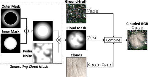
Next, a real cloud image, labeled ‘Clouds’ in Figure 1, is used. It is a four-band image extracted from a cloud image of the Landsat 8 Cloud Cover Assessment Validation Data (U.S. Geological Survey 2016) dataset obtained with the Landsat 8 Operational Land Imager (OLI) and Thermal Infrared Sensor (TIRS). The three RGB wavelengths are in the range 0.45–0.67 $\mu$m, while the NIR band wavelength is in the range 0.85–0.88 $\mu$m. The RGB and NIR bands are denoted $c_{\mathrm{R}\mathrm{G}\mathrm{B}}$ and $c_{\mathrm{N}\mathrm{I}\mathrm{R}}$, respectively. The clouded RGB image is obtained by

(1) $x_{\mathrm{R}\mathrm{G}\mathrm{B}}=(1-y_{\mathrm{C}\mathrm{M}}^{(3)})\odot y_{\mathrm{R}\mathrm{G}\mathrm{B}}^{\tau }+y_{\mathrm{C}\mathrm{M}}^{(3)}\odot c_{\mathrm{R}\mathrm{G}\mathrm{B}},$(1)

where $\odot$ is the element-wise product and $y_{\mathrm{C}\mathrm{M}}^{(3)}$ is comprised of three copies of $y_{\mathrm{C}\mathrm{M}}$, i.e. $y_{\mathrm{C}\mathrm{M}}^{(3)}=[y_{\mathrm{C}\mathrm{M}},y_{\mathrm{C}\mathrm{M}},y_{\mathrm{C}\mathrm{M}}]$. NIR wavelengths in 0.77–0.90 $\mu$m are longer than the optical RGB wavelengths in 0.45–0.69 $\mu$m and thus are known to have filmy cloud penetration capabilities. Therefore, the clouded NIR image is expected to carry additional information on the scenery beneath the cloud. To model this, we introduce the NIR cloud penetrability parameter denoted ${\eta }_{\mathrm{N}\mathrm{I}\mathrm{R}}\in [0,1]$, where ${\eta }_{\mathrm{N}\mathrm{I}\mathrm{R}}=0$ corresponds to no auxiliary information being provided. We then adapt the cloud insertion technique to synthesise clouded NIR images as follows:

(2) $x_{\mathrm{N}\mathrm{I}\mathrm{R}}=[1-(1-{\eta }_{\mathrm{N}\mathrm{I}\mathrm{R}})y_{\mathrm{C}\mathrm{M}}]\odot y_{\mathrm{N}\mathrm{I}\mathrm{R}}^{\tau }+(1-{\eta }_{\mathrm{N}\mathrm{I}\mathrm{R}})y_{\mathrm{C}\mathrm{M}}\odot c_{\mathrm{N}\mathrm{I}\mathrm{R}}.$(2)

4. Proposed method

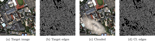
MEcGANs are aimed to provide enhanced object restoration capabilities in built-up areas covered by clouds. For this, they extend McGANs by considering edge-filtered clouded or target RGB images as additional input to the discriminator. Target RGB images of built-up areas are characterised by many edges in their edge-filtered counterparts, see Figure 2(a,b), while cloud-covered parts of these areas result in black, edge-free spots with edge-rich surroundings, see Figure 2(c,d). Thus, the generator is forced to exploit the extra information contained in co-registered clouded NIR images to generate cloud-free RGB images and their edge-filtered versions that resemble the ones from the target domain, i.e. the edge-free parts need to be filled with edges.

Figure 2. Example of target and clouded RGB images with their corresponding edge-filtered variants.

MEcGANs consists of a generator $G$ and a discriminator $D$ schematically depicted in Figure 3. The generator is fed with $x=(x_{\mathrm{R}\mathrm{G}\mathrm{B}},x_{\mathrm{N}\mathrm{I}\mathrm{R}})$ as in Enomoto et al. (2017), but here $x_{\mathrm{N}\mathrm{I}\mathrm{R}}$ is clouded. $G$ produces a pair $\hat{y}=({\hat{y}}_{\mathrm{R}\mathrm{G}\mathrm{B}},{\hat{y}}_{\mathrm{C}\mathrm{M}})$ of generated cloud-free RGB image (${\hat{y}}_{\mathrm{R}\mathrm{G}\mathrm{B}}$) and a corresponding cloud mask (${\hat{y}}_{\mathrm{C}\mathrm{M}}$), i.e. $\hat{y}:=G(x)$.

The generated or target RGB image is processed by edge detection, i.e. application of a Canny edge detection filter, denoted $\mathrm{e}(\cdot )$ (Canny 1986). The discriminator $D$ takes three inputs, instantiated in two different ways, as we explain here. The first parameter $x$, is always the clouded pair of RGB and NIR images. The second two parameters are either instantiated as $\hat{y},\hat{z}$ or $y^{\tau },z^{\tau }$. The former pair represents generated images and edge-filtered counterparts, i.e. $\hat{z}:=\mathrm{e}({\hat{y}}_{\mathrm{R}\mathrm{G}\mathrm{B}})$. The latter pair is the corresponding target images: the ground truth $y^{\tau }=(y_{\mathrm{R}\mathrm{G}\mathrm{B}}^{\tau },y_{\mathrm{c}\mathrm{l}\mathrm{o}\mathrm{u}\mathrm{d}}^{\tau })$ where $y_{\mathrm{c}\mathrm{l}\mathrm{o}\mathrm{u}\mathrm{d}}^{\tau }=y_{\mathrm{C}\mathrm{M}}\odot c_{\mathrm{N}\mathrm{I}\mathrm{R}}$ is a monochromatic cloud image, and $z^{\tau }:=\mathrm{e}(y_{\mathrm{R}\mathrm{G}\mathrm{B}}^{\tau })$ representing the ground truth after applying edge filtering. The novelty compared to Enomoto et al. (2017) is the introduction of the third edge-filtered parameter.

Given any $D$, generator $G$ is trained to minimise its loss function ${\mathbb{E}}_x[log(1-D(x,\hat{y},\hat{z}))]+\lambda {\mathcal{L}}_{\mathrm{L}1}(G)$, where $\lambda$ is a scaling factor and

(3) ${\mathcal{L}}_{\mathrm{L}1}(G)={\mathbb{E}}_{x,y^{\tau }}[\parallel y^{\tau }-\hat{y}{\parallel }_1]$(3)

is an L1 loss which imposes less blurring. As Enomoto et al., we set $\lambda =100$. Simultaneously, the training criterion for $D$, given any $G$, is to maximise the loss function

(4) $\mathcal{L}(G,D)={\mathbb{E}}_{x,y^{\tau }}[logD(x,y^{\tau },z^{\tau })]+{\mathbb{E}}_x[log(1-D(x,\hat{y},\hat{z}))].$(4)

Thus, $D$ and $G$ play a min-max game with the final objective to find an optimal generator

(5) $G^{\ast }=arg\underset{G}{min}\underset{D}{max}\mathcal{L}(G,D)+\lambda {\mathcal{L}}_{\mathrm{L}1}(G).$(5)

Apart from the modifications described above, we use the original McGAN architecture (Enomoto et al. 2017). In general, the layers of $G$ and $D$ are built as follows. They consist of a convolution (Conv) or a deconvolution (DeConv) component specified by four parameters: number of channels, kernel size, stride, and padding. The components are followed by a BatchNormalisation (BNorm) or a Dropout with ratio $0.5$ (Drop) module. Finally, the ReLU or LeakyReLU (LReLU) activation function is applied. $G$ has exactly the same encoder-decoder structure with skip connections as the generator of McGANs. Its input and output are $x=(x_{\mathrm{R}\mathrm{G}\mathrm{B}},x_{\mathrm{N}\mathrm{I}\mathrm{R}})$ and $\hat{y}=({\hat{y}}_{\mathrm{R}\mathrm{G}\mathrm{B}},{\hat{y}}_{\mathrm{C}\mathrm{M}})$, respectively. The architecture of $D$ is provided in Table 1.

Figure 3. Network architecture of the MEcGans framework.

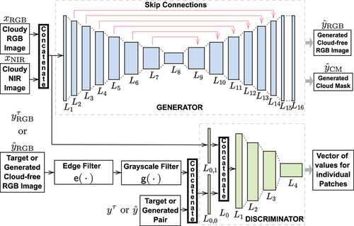
Table 1. Discriminator architecture

Discriminator $D$
In:	$(x,\hat{y}=({\hat{y}}_{\mathrm{R}\mathrm{G}\mathrm{B}},{\hat{y}}_{\mathrm{C}\mathrm{M}}),\hat{z})$ or
Layer	Architecture
$L_{0,0}$	$\mathrm{C}\mathrm{o}\mathrm{n}\mathrm{v}(32,4,2,1)(x)$; LReLU
$L_{0,1}$	$\mathrm{C}\mathrm{o}\mathrm{n}\mathrm{v}(32,4,2,1)((\hat{y},\hat{z})\mathrm{o}\mathrm{r}(y^{\tau },z^{\tau }))$;
	LReLU
$L_1$	$\mathrm{C}\mathrm{o}\mathrm{n}\mathrm{v}(128,4,2,1)$; BNorm; LReLU
$L_2$	$\mathrm{C}\mathrm{o}\mathrm{n}\mathrm{v}(256,4,2,1)$; BNorm; LReLU
$L_3$	$\mathrm{C}\mathrm{o}\mathrm{n}\mathrm{v}(512,4,2,1)$; BNorm; LReLU
$L_4$	$\mathrm{C}\mathrm{o}\mathrm{n}\mathrm{v}(1,3,1,1)$;
Out:	Vector of values for image patches

5. Evaluation

We evaluate MEcGANs against McGANs on two different datasets. For fairness of comparison, the McGANs are supplied with clouded NIR images and not cloud-free ones as in the original study.

Our hypothesis is that with the additional edge-filtered input, the discriminator of MEcGANs can more easily distinguish between target and generated input and thus drive the generator toward more exact reconstruction of cloud-covered areas. To verify this, we consider a dataset of images mainly containing built-up areas with their edge-filtered versions having many edges as, for example, in Figure 2(b). The dataset consists of $2039$ training and $160$ images obtained by cropping selected images of Berlin city from WorldView-2 European Cities. To assure that mainly images with built-up areas are included, we proceed as follows. First, we cluster the images with the uniformisation approach of Enomoto et al. (2017) utilising AlexNet to extract for each image a 4096-dimensional feature vector, which is then mapped with t-SNE to 2D space for clustering on a $32\times 32$ grid. However, differently from Enomoto et al. (2017), we do not sample uniformly from this space. Instead, based on visual inspection of the placement of the images on the grid, we specify a rectangular region of the grid where the built-up area-intensive images are placed and we form the ‘Berlin dataset’ from all the images in this region. From the total number of $2199$ images, we sample $160$ test images and the remaining $2039$ are used for training. The total size of the Berlin dataset is chosen to be similar to the size of the dataset used in Enomoto et al. (2017).

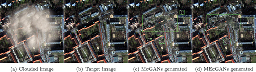
McGANs and MEcGANs are trained for $500$K iterations with ${\eta }_{\mathrm{N}\mathrm{I}\mathrm{R}}=1\mathrm{\%}$ and evaluated in terms of ${\mathcal{L}}_{\mathrm{L}1}$ on the test images after each $50$K iterations. We compare the results obtained with the best models of McGANs and MEcGANs, which in both cases were the ones at $500$K iterations. Although both methods generate images of similar quality at first sight, a careful inspection reveals that MEcGANs outperforms McGANs. To see this, we visualise the differences as follows. First, we compute the difference images between the target cloud-free image and the generated images of McGANs and MEcGANs with the structural_similarity function of the scikit-image Python package (Van der Walt et al. 2014). Next, with the OpenCV library (Bradski 2000), we compute the difference contours, i.e. contours of the regions where the McGANs- and MEcGANs-generated images differ with respect to the target image and the areas (in pixel) of these contours. Finally, we compute the bounding boxes of the contours for visualisation purposes. The obtained results for an example test image are shown in Figure 4, where the total difference contours area is reduced by MEcGANs from $3501$ px (McGANs) to $2955$ px (MEcGANs)².

Figure 4. Example of Berlin dataset test image results with ${\eta }_{\mathrm{N}\mathrm{I}\mathrm{R}}=1\mathrm{\%}$. for the generated images (c)-(d), the differences w.r.t. the target image (b) are highlighted by the contours (white) and their bounding boxes (green).

We perform a quantitative evaluation of the generated images. First, we consider the total difference contours area (TDCA) for the Berlin dataset test images with ${\eta }_{\mathrm{N}\mathrm{I}\mathrm{R}}=1\mathrm{\%}$, which is $744490$ px and $716115$ px for McGANs and MEcGANs, respectively. MEcGANs provides an improvement of $3.8\mathrm{\%}$. Notice that this result has to be interpreted in the light of the fact that MEcGANs is expected to provide improvement only in areas covered by filmy clouds, which usually constitutes a small portion of the total clouded area. Hence, we consider the improvement as significant. In terms of TDCA for individual test images, MEcGANs outperforms McGANs on $99$ images.

Next, we consider in this study three commonly used metrics: Peak Signal-to-Noise Ratio (PSNR), Structural Similarity Index (SSIM), and Spatial Correlation Coefficient (SCC), where target images are used as reference. MEcGANs outperforms McGANs with respect to all of them. Specifically, MEcGANs is better in terms of PSNR on $82$ test images. With respect to SSIM and SCC, which are considered more reliable image quality indicators, MEcGANs is respectively better on $101$ and $146$ test images. The medians of the metrics are provided in Table 2, while the boxplot summaries of SSIM and SCC are shown in Figure 5. The median and the mean of the two metrics are consistently higher for MEcGANs, see Figure 5(a,b). The same remains true for the edge-filtered versions of the generated images, see Figure 5(c,d). MEcGANs gain higher SSIM and SCC values for $130$ and $128$ edge-filtered test images, respectively.

Figure 5. Boxplot summary of SSIM and SCC results on the Berlin dataset test images (a)-(b) and their edge-filtered versions (c)-(d). the boxes extend from the lower to upper quartile values of the data, with an orange line at the median and a green triangle at the mean. the positions of whiskers and flier points are determined by Tukey’s original boxplot definition.

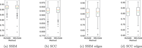
Table 2. Medians of the metrics on the Berlin dataset for different values of ${\eta }_{NIR}$. McG. and MEcG. stand for McGans and MEcGans, respectively; $\mathrm{△}$ is the percentage increase obtained by MEcGans w.R.t McGans

Medians	${\eta }_{\mathrm{N}\mathrm{I}\mathrm{R}}=0.1\mathrm{\%}$			${\eta }_{\mathrm{N}\mathrm{I}\mathrm{R}}=0.5\mathrm{\%}$			${\eta }_{\mathrm{N}\mathrm{I}\mathrm{R}}=1\mathrm{\%}$
	PSNR	SSIM	SCC	PSNR	SSIM	SCC	PSNR	SSIM	SCC
McG.	25.402	0.935	0.930	24.978	0.928	0.927	24.862	0.926	0.929
MEcG.	25.636	0.938	0.943	25.358	0.932	0.938	25.109	0.928	0.933
$\mathrm{\Delta }[\mathrm{\%}]$	0.92	0.38	1.48	1.52	0.43	1.25	0.99	0.25	0.37

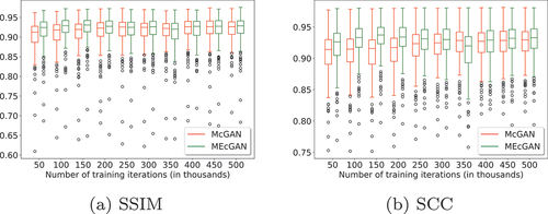
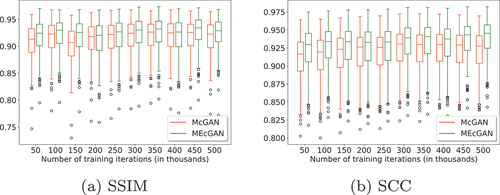
Moreover, as can be seen in Figure 6 which presents the number of test images on which MEcGANs are better/worse compared to McGANs in terms of SSIM, SCC, and TDCA after each 50 K iterations, the better performance of MEcGANs is consistent throughout the whole training procedure, with two exceptions at 350K and 400K. The boxplot summaries of the SSIM and SCC metrics throughout the training are shown in Figure 7. Furthermore, the SSIM and SCC results obtained for edge-filtered versions of the generated images show full supremacy of MEcGANs throughout the training (data available online via Mizera (2021)).

Figure 6. Number of Berlin dataset test images on which MEcGans performed better (blue bars) and worse (orange bars) with respect to McGans after each $50$k iterations of training.

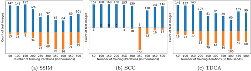
Figure 7. Comparison of MEcGans and McGans performance on the test images of the Berlin dataset throughout training.

We proceed with the evaluation by compiling a second, smaller dataset of approximately half the size of the Berlin dataset to investigate the robustness of MEcGANs with respect to training dataset size and to check how MEcGANs compares to McGANs in cases where no large training datasets are available. Again, we aim to focus on built-up areas, but we use a slightly different approach than for the Berlin dataset. We select satellite images of Paris from WorldView-2 European Cities that contain built-up areas to a large extent. We crop them into pairs of RGB and NIR images and apply the original uniformisation method of Enomoto et al. (2017) to uniformly sample 1000 positions in a 32 × 32 grid. This gives a total number of 1045 images (800 training and 245 test images) forming the ‘Paris dataset’ mainly consisting of built-up area images plus a small portion of other types of images.

As before, we train the two methods for 500K iterations with ${\eta }_{\mathrm{N}\mathrm{I}\mathrm{R}}=1\mathrm{\%}$ . In both cases, the best fitted models in terms of ${\mathcal{L}}_{\mathrm{L}1}$ are obtained at 500 K iterations. Example results are presented in Figure 8. The difference contours areas are reduced by MEcGANs from 2549.5 to 1942.5 (top row) and from 3058.5 to 2497.5 (bottom row). Cumulatively on all the 245 test images, TDCA is reduced from 1,084,694 (McGANs) to 1,015,855 (MEcGANs), which gives an improvement of 6.3%. Considering individual test images, MEcGANs outperforms McGANs on 215 of them. With respect to PSNR, SSIM, and SCC metrics, MEcGANs surpasses McGANs on 208, 233, and 244 test images, respectively. The medians of these metrics on the whole test subset are provided in Table 3. The boxplot summaries of SSIM and SCC are provided in Figure 9. Again, the median and the mean of the two metrics are consistently higher for MEcGANs both for the original and edge-filtered variants. In the case of edge-filtered test images, MEcGANs gained higher SSIM and SCC values for all 245 images.

Figure 8. Excerpt of Paris dataset testimage results with . for the generated images(c)-(d), the differences w.r.t. the target image (b) are highlighted by thecontours (white) and their bounding boxes (green).

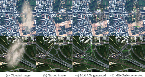
Figure 9. Boxplot summary of SSIM and SCC results on the Paris dataset test images (a)-(b) and their edge-filtered versions (c)-(d). the boxes extend from the lower to upper quartile values of the data, with an orange line at the median and a green triangle at the mean. the positions of whiskers and flier points are determined by Tukey’s original boxplot definition.

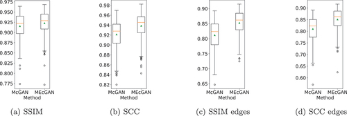
Table 3. Medians of the metrics on the Paris dataset for different values of ${\eta }_{\mathrm{N}\mathrm{I}\mathrm{R}}$. McG. and MEcG. stand for McGans and MEcGans, respectively; $\mathrm{△}$ is the percentage increase obtained by MEcGans w.R.t McGans

Medians	${\eta }_{\mathrm{N}\mathrm{I}\mathrm{R}}=0.1\mathrm{\%}$			${\eta }_{\mathrm{N}\mathrm{I}\mathrm{R}}=0.5\mathrm{\%}$			${\eta }_{\mathrm{N}\mathrm{I}\mathrm{R}}=1\mathrm{\%}$
	PSNR	SSIM	SCC	PSNR	SSIM	SCC	PSNR	SSIM	SCC
McG.	23.790	0.926	0.933	23.755	0.925	0.928	23.610	0.922	0.928
MEcG.	24.645	0.943	0.947	24.299	0.937	0.946	24.010	0.929	0.945
$\mathrm{\Delta }[\mathrm{\%}]$	3.59	1.86	1.46	2.29	1.28	1.94	1.70	0.72	1.90

As in the case of the Berlin dataset, also for the Paris dataset the supremacy of MEcGANs is consistent throughout the training as shown in Figure 10 and 11.

Figure 10. Number of Paris dataset test images on which MEcGans performed better (blue bars) and worse (orange bars) with respect to McGans after each $50.$k iterations of training.

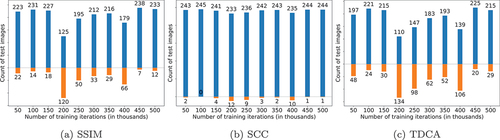
Figure 11. Comparison of MEcGans and McGans performance on the test images of the Paris dataset throughout training.

Since we were unable to find any suitable physical model of NIR penetration of clouds in the literature, we introduced the ${\eta }_{\mathrm{N}\mathrm{I}\mathrm{R}}$ parameter to simulate the enhanced cloud penetrability by NIR. Being aware that the model is physically not fully accurate, we proceed to evaluate the robustness of MEcGANs in cases where the NIR information is reduced. To this aim, we investigate the sensitivity of our method to ${\eta }_{\mathrm{N}\mathrm{I}\mathrm{R}}$ by repeating the experiments on the two datasets with ${\eta }_{\mathrm{N}\mathrm{I}\mathrm{R}}$ set to 0.5% and 0.1%. The TDCA values are provided in Table 4, while the medians for the PSNR, SSIM, and SCC metrics are given in Tables 2 and 3 for the Berlin and Paris datasets, respectively. The results show that MEcGANs provides a persistent improvement in terms of all the considered metrics across the two datasets for all the ${\eta }_{\mathrm{N}\mathrm{I}\mathrm{R}}$ values. In consequence, the performance of our method is robust with respect to different values of ${\eta }_{\mathrm{N}\mathrm{I}\mathrm{R}}$ and therefore we would expect MEcGANs to perform well for more physically accurate NIR penetrability models, too.

Table 4. TDCA for the two datasets with different ${\eta }_{\mathrm{N}\mathrm{I}\mathrm{R}}$ values. McG. and MEcG. stand for McGans and MEcGans, respectively; $\mathrm{△}$ is the percentage decrease obtained by MEcGans with respect to McGans

TDCA	${\eta }_{NIR}=0.1\mathrm{\%}$		${\eta }_{\mathrm{N}\mathrm{I}\mathrm{R}}=0.5\mathrm{\%}$		${\eta }_{\mathrm{N}\mathrm{I}\mathrm{R}}=1\mathrm{\%}$
	Berlin	Paris	Berlin	Paris	Berlin	Paris
McG.	698543.5	1058566.5	706482.5	1055105.0	744490.0	1084694.0
MEcG.	657507.5	907790.0	666663.5	929048.0	716115.0	1015855.0
$\mathrm{\Delta }[\mathrm{\%}]$	5.9	14.2	5.6	11.9	3.8	6.3

6. Conclusions and future work

We propose MEcGANs, a new framework for cloud removal in satellite imagery which extends the method of Enomoto et al. (2017) in two significant ways. Firstly, the new discriminator differentiates between target and generated cloud-free RGB images by additionally considering edge-filtered inputs. This drives the generator learning toward improved reconstruction of cloud-covered objects. Secondly, our approach is more realistic in that it takes as input clouded NIR images. The better translucency of NIR wavelengths with respect to the visible light spectrum is modeled by introducing an NIR cloud penetrability parameter.

We consider two datasets of synthesised clouded RGB and clouded NIR images: one of size 2199 and the other of size 1045. With respect to Enomoto et al. (2017), instead of simply generating Perlin noise, we employ an improved, state-of-the-art cloud insertion technique of Rafique, Blanton and Jacobs (2019), which provides more realistic clouded images by making fewer assumptions on the observation model and the physics of clouds. The datasets consists mostly of images of urban areas, since our focus is on object reconstruction.

We compare the performance of MEcGANs versus McGANs by computing the areas of the difference regions in the generated cloud-free images with respect to the corresponding target images. The results demonstrate the superiority of MEcGANs in comparison to McGANs on two different datasets – a large dataset and a small dataset. It is evident that MEcGANs provides an improvement in the regions obscured by filmy clouds. These results are supported by quantitative comparison analysis, which is based on three metrics commonly considered in the context of image restoration, i.e. Peak Signal-to-Noise Ratio, Structural Similarity Index, and Spatial Correlation Coefficient. Furthermore, the obtained results show that MEcGANs are robust with respect to the training dataset size. Interestingly, the relative improvements, as measured by the relative decrease in the total difference area, and the average gains of the three considered metrics, are the greatest in the case of the small dataset. This suggests that MEcGANs are suitable when training data is limited.

Since we could not find a proper physical model for enhanced NIR cloud penetrability in the literature, we simulate it by introducing a NIR cloud penetrability parameter and we investigate the robustness of the performance of MEcGANs for various values of this parameter. Experimental results confirm that MEcGANs are robust and can capture and exploit even a weak NIR ‘signal’ providing information on the scene underneath the clouds. We therefore expect it to perform well in the case of more sophisticated and accurate models of NIR cloud penetrability.

We believe that MEcGANs are general in nature and can be applied to sources of auxiliary information other than NIR. As future work, we plan to consider datasets where clouds are not synthetic and to investigate the impact of replacing NIR with SAR images. That would involve evaluating MEcGANs on data consisting of aligned triplets of target RGB, clouded RGB, and NIR or SAR images. This is a separate problem requiring methods to properly align images of different types acquired at different times.

Disclosure statement

No potential conflict of interest was reported by the author(s).

Notes

1. For reproducibility purposes, all cropped images are made available (Mizera 2021).

2. Due to space limitation, the full set of results is available online via (Mizera 2021).

References

- Bradski, G. 2000. “The OpenCv Library.” Dr. Dobb’s Journal: Software Tools for the Professional Programmer 25 (11): 120.
- Canny, J.F. 1986. “A Computational Approach to Edge Detection.” IEEE Transactions on Pattern Analysis and Machine Intelligence 8 (6): 679. doi:https://doi.org/10.1109/TPAMI.1986.4767851.
- Enomoto, K., K. Sakurada, W. Wang, H. Fukui, M. Matsuoka, R. Nakamura, and N. Kawaguchi. 2017. “Filmy Cloud Removal on Satellite Imagery with Multispectral Conditional Generative Adversarial Nets.” In IEEE Conference on Computer Vision and Pattern Recognition Workshops (CVPR) Workshop, 48–56. Honolulu, HI, USA.
- ESA (European Space Agency). 2020. “WorldView-2 European Cities.” DigitalGlobe Inc. (2020), provided by European Space Imaging. Accessed December 2021. https://earth.esa.int/eogateway/catalog/worldview-2-european-cities
- Gao, J., Q. Yuan, J. Li, H. Zhang, and X. Su. 2020. “Cloud Removal with Fusion of High Resolution Optical and SAR Images Using Generative Adversarial Networks.” Remote Sensing 12 (1): 191.
- Goodfellow, I., J. Pouget-Abadie, M. Mirza, B. Xu, D. Warde-Farley, S. Ozair, A. Courville, and Y. Bengio. 2014. “Generative Adversarial Nets.” In NIPS'14: Proceedings of the 27th International Conference on Neural Information Processing Systems, 2672–2680. Montreal, Canada.
- Grohnfeldt, C., M. Schmitt, and X. Zhu. 2018. “A Conditional Generative Adversarial Network to Fuse Sar and Multispectral Optical Data for Cloud Removal from Sentinel-2 Images.” In IEEE International Geoscience and Remote Sensing Symposium (IGARSS), 1726–1729. Valencia, Spain.
- Isola, P., J.-Y. Zhu, T. Zhou, and A.A. Efros. 2017. “Image-To-Image Translation with Conditional Adversarial Networks.” In IEEE Conference on Computer Vision and Pattern Recognition (CVPR), 5967. Honolulu, Hawaii.
- Li, J., Z. Wu, Z. Hu, J. Zhang, M. Li, L. Mo, and M. Molinier. 2020. “Thin Cloud Removal in Optical Remote Sensing Images Based on Generative Adversarial Networks and Physical Model of Cloud Distortion.” ISPRS Journal of Photogrammetry and Remote Sensing 166: 373.
- Meraner, A., P. Ebel, X.X. Zhu, and M. Schmitt. 2020. “Cloud Removal in Sentinel-2 Imagery Using a Deep Residual Neural Network and SAR-Optical Data Fusion.” ISPRS Journal of Photogrammetry and Remote Sensing 166: 333.
- Mirza, M. and S. Osindero. 2014. ”Conditional Generative Adversarial Nets.” arXiv: 1411.1784.
- Mizera, A. 2021. “Github Repository of MEcGans.” https://github.com/andrzejmizera/MEcGANs.
- Perlin, K. 2002. “Improving Noise.” ACM Transactions on Graphics 21 (3): 681.
- Radford, A., L. Metz, and S. Chintala. 2015. “Unsupervised Representation Learning with Deep Convolutional Generative Adversarial Networks.” arXiv: 1511.06434.
- Rafique, M.U., H. Blanton, and N. Jacobs. 2019. “Weakly Supervised Fusion of Multiple Overhead Images.” In IEEE/CVF Conference on Computer Vision and Pattern Recognition Workshops (CVPRW), 1479. Long Beach, CA, USA.
- Schläpfer, D., R. Richter, and P. Reinartz. 2020. “Elevation-Dependent Removal of Cirrus Clouds in Satellite Imagery.” Remote Sensing 12 (3): 494.
- Singh, P. and N. Komodakis. 2018. “Cloud-GAN: Cloud Removal for Sentinel-2 Imagery Using a Cyclic Consistent Generative Adversarial Networks.” In IEEE International Geoscience and Remote Sensing Symposium (IGARSS), 1772. Valencia, Spain.
- U.S. Geological Survey. 2016. “L8 Biome Cloud Validation Masks.”U.S. Geological Survey, data release .https://doi.org/http://dx.doi.org/10.5066/F7251GDHdoi:10.5066/F7251GDH (accessed December 2021).
- Van der Walt, S., J.L. Schönberger, J. Nunez-Iglesias, F. Boulogne, J.D. Warner, N. Yager, E. Gouillart, T. Yu, and the scikit-image contributors. 2014. ”Scikit-Image Contributors. Scikit-Image: Image Processingin Python.” PeerJ 2: e453.
- Zhang, H., V. Sindagi, and V.M. Patel. 2020. “Image De-Raining Using a Conditional Generative Adversarial Network.” IEEE Transactions on Circuits and Systems for Video Technology 30 (11): 3943.