Assessing vegetation traits estimates accuracies from the future SBG and biodiversity hyperspectral missions over two Mediterranean Forests

ABSTRACT

The estimation and mapping of vegetation traits from satellite hyperspectral imagery is entering a new era, as multiple missions have recently started and more are currently in preparatory phase. With expected ground sampling distances (GSD) ranging from 8 to 30 m, these missions could complement each other, especially over spatially heterogeneous environments where the canopy cover (CC) is low. This study focused on the retrieval of five vegetation traits (gap fraction, leaf chlorophylls (C${ }_{ab}$) and carotenoids (Car) contents, equivalent water thickness, and leaf mass per area) of two Mediterranean-climate forests from AVIRIS-Classic (AVIRIS-C), synthetic Biodiversity, and synthetic Surface Biology and Geology (SBG) missions with 18 m, 8 m, and 30 m GSD, respectively, using a hybrid method. The synthetic SBG images were provided by NASA, while the Biodiversity images were generated from airborne AVIRIS-Next Generation hyperspectral imagery. Partial least-square regressors were trained over the outputs of the DART model to estimates vegetation traits. Estimated accuracies were assessed, when possible, by comparison with in situ measurements. We showed that estimated accuracy of gap fraction was similar between AVIRIS-C and SBG (RMSE of 0.09, R${ }^2$ of 0.8 and RMSE of 0.07, R${ }^2$ of 0.59, respectively). Leaf traits estimated accuracies were also similar between these two sensors, but only acceptable for C${ }_{ab}$ and Car ($\sim$ 7.5 μg.cm${ }^{-2}$ RMSE for C${ }_{ab}$, $\sim$ 1.65 μg.cm${ }^{-2}$ RMSE for Car), especially over the densest parts of the canopy. When comparing estimates obtained from Biodiversity and SBG imagery, it appeared that the denser the canopy, the more estimates from both sensors were in agreement for all leaf traits (for instance, C${ }_{ab}$, R${ }^2$ was 0.2 for 30% $\le$ CC $\le$ 50% and 0.48 for CC $\ge$ 80%). The results show that (i) SBG imagery should lead to estimated accuracies similar to AVIRIS-C, with acceptable performances over dense canopies, and that (ii) Biodiversity imagery has a high potential to map vegetation traits over any canopy no matter its sparsity, as individual tree crowns are mostly resolved at an 8 m GSD.

KEYWORDS:

• Imaging spectroscopy
• hybrid method
• DART
• PLSR
• vegetation traits

1. Introduction

Even though they only cover 2% of land surfaces, the Mediterranean ecoregions are home to 20% of global plant species (Cowling et al. 1996) which puts them among the major biodiversity hotspots (Myers et al. 2000). This diversity varies over a great range of environments: indeed, while true forests with closed canopies do exist in these ecosystems, open canopies are a common occurence (Gauquelin et al. 2018) due to the historically strong climatic and anthropogenic pressures (Scarascia-Mugnozza et al. 2000). However, temperature and aridity are expected to rise considerably by 2100 (Somot et al. 2008), significantly endangering their biodiversity (Sala et al. 2000). The ability to monitor the health status of Mediterranean ecosystems is therefore crucial to possibly guide conservation policies.

Due to their ability to cover large swathes almost continuously, satellite-based remote sensing methods are expected to have an important role in future global monitoring efforts, and the concept of satellite-specific Essential Biodiversity Variables has recently been defined (Pettorelli et al. 2016). Several hyperspectral missions, such as EnMAP (Guanter et al. 2015), CHIME (Rast et al. 2019), SHALOM (Feingersh and Ben Dor 2015), SBG (inheritor of HyspIRI (Lee et al. 2015)), Biodiversity (inheritor of HypXIM (Carrere et al. 2013)) or PRISMA Second generation, are in preparation, prefiguring a new era concerning hyperspectral remote sensing of vegetation. While most satellite sensors should have a Ground Sampling Distance (GSD) of 30 m, SHALOM and Biodiversity are expected to have a GSD of 10 and 8 m, respectively, which would make it possible to better identify canopy structure, especially concerning open forests, at the cost of a lower Signal-to-Noise Ratio (SNR) and a lower temporal resolution. Assessing retrieval performances of vegetation parameters from images taken by low and medium GSD satellite sensors over open and closed canopies will help understand how they complement each other as well as their respective limitations.

Various methods exist to retrieve these vegetation parametres from hyperspectral images, usually categorized into four main families (Verrelst et al. 2015). Parametric and non-parametric empirical-statistical methods, where a model is fitted using data collected in situ, have been used with great success: for instance, Dana Chadwick and Gregory (2016) demonstrated that the leaf content in a variety of leaf biochemicals could be obtained from high-resolution hyperspectral images using Partial-Least-Square Regression (PLSR) trained on collected data. Similarly, Siegmann and Jarmer (2015) obtained consistent results estimating the Leaf Area Index (LAI) through PLSR over croplands. In contrast, physically based methods usually rely on time-consuming Look-Up Table (LUT)-based inversion of a Radiative Transfer Model (RTM), which have for instance been shown to adequately estimate LAI and needle Chlorophylls a+b content (C${ }_{ab}$) of sparse conifer forests (Darvishzadeh et al. 2019; Zarco-Tejada et al. 2019) when using Sentinel-2 images. Finally, the so-called hybrid methods consist of fitting models using the outputs of a RTM. By combining the generic properties of RTM with the efficiency of empirical-statistical methods, they could be the ideal methods for processing global satellite data in the near future Verrelst et al. (2015); Berger et al. (2018). Malenovský et al. (2013) demonstrated that needle C${ }_{ab}$ could be retrieved from sub-metre resolution hyperspectral images by training an Artifical Neural Network (ANN) over the outputs of the DART model (Gastellu-Etchegorry et al. 2015), outperforming the other Vegetation Indexes (VI) used in their study in terms of estimation accuracy. More recently, Ali et al. (2020) compared the performances of LUT-based and various non-parametric methods based on the outputs of the RTM to estimate LAI and C${ }_{ab}$ of mixed forest stands from Sentinel-2 imagery, and found that most hybrid methods presented accuracies similar to those of the LUT inversion at a fraction of the time cost, highlighting their potential for future operational use.

The goal of the present study was to assess the estimation accuracies that could be expected from hyperspectral images acquired by SBG and Biodiversity over heterogeneous canopies such as those present in Mediterranean ecosystems and the evolution of these estimations with the openness of the canopy.

2. Materials and methods

2.1. Study sites

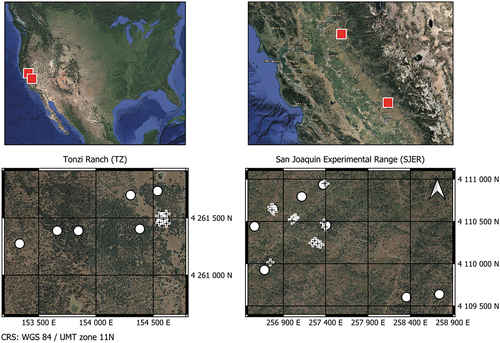
The study sites are located in the lower foothills of the Sierra Nevada (Tonzi Ranch (TZ), latitude: 38.5 °N; longitude: 121.0 °W, San Joachin Experimental Range (SJER), latitude: 37.1 °N; longitude: 119.7 °W). They are categorized as grass-oak pines woodlands and both have a Mediterranean climate with hot, dry summers and mild, wet winters. The canopy of TZ is dominated by blue oaks (Quercus douglasii (QUDO)) with a small population of grey pine (Pinus sabiniana – PISA), while the one of SJER mostly consists in QUDO, interior live oaks (Quercus wislizeni (QUWI)) and PISA. The period of activity of QUDO starts in April and ends around November, while QUWI and PISA are evergreen species. The understory of both sites is composed of annual grass species active from December to May and dry during the summer period. For TZ the average LAI is 0.8 m${ }^2$.m${ }^{-2}$ and the mean canopy cover 47% (Kobayashi et al. 2013), with mean annual tempatures and precipitations of 16.5°C and 562 mm, respectively, and a soil classified as Auburn very rocky silt loam soil (Chen et al. 2008). For SJER, the canopy cover is about 30%, with average temperatures and annual precipitations of 16.5°C and 485 mm, respectively. The soil type at SJER is classified as Vista rocky coarse sandy loam (Tate et al. 2004). Aerial views of the sites as well as location of the field measurements considered in this study are given in Figure 1.

Figure 1. Location and aerial views of Tonzi Ranch and the San Joaquin Experimental Range. Circles and crosses indicate the locations where Digital Hemispherical Photographs (DHP) and leaf collection took place, respectively. Images obtained from Google Maps.

2.2. Field data

Field data were collected coincidentally with the overflights of NASA Hyperspectral Infrared Imager (HyspIRI) Mission Study Airborne Campaigns that occured between Summer 2013 and Fall 2014.

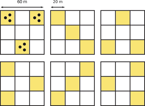
Several digital hemispherical photographs (DHP) were collected over 16 60 m $\times$ 60 m plots within the study sites with the objective to cover various levels of CC and species composition. Within each plot, nine DHP were taken using a Nikon Coolpix 4300 camera post sunset so that the sky illumination was uniform. Figure 2 shows how the DHP were taken over the 16 plots. DHP were processed using the CAN-EYE (https://www6.paca.inrae.fr/can-eye) software, which calculated the Gap Fraction at an angular resolution of 2.5° and within a circle of interest of 65°.

Figure 2. Sampling patterns used for the collection of the DHP over the 60 m $\times$ 60 m plots.

Leaf collections were made from the upper, sunlit portion of the crowns as high as possible on the eastern and western sides, occurred coincident with the overflights. Leaves were wrapped in foil to prevent degradation from sunlight, and stored on blue ice before being transferred to a lab refrigerator until laboratory measurements. Measurements occured within 48 hours of collection. Leaf samples were frozen in liquid nitrogen for a short time until lyophilized. The extraction was done in 14 mL of 90% acetone for 48 hours, which yielded enough solvent extract to obtain 3.5 mL samples for each tree. UV/Vis spectrophotometer runs were done with concentrations of 23 mg/mL for chlorophylls and 8 mg/mL for carotenoids as standards. Absorbance of the solution was measured at 0.470, 0.662, 0.645, and 0.710 μm. Chlorophylls and carotenoids concentrations of the solution were measured according to the methodology described by Lichtenthaler (1987) and Lichtenthaler and Buschmann (2001) with a dilution factor equal to 3.5, to finally obtain chlorophylls a + b and carotenoid content per unit of leaf area (μg.cm${ }^{-2}$). Table 1 indicates the number of trees sampled during the leaf collection and the number of DHP plots, and their main characteristics.

Table 1. Data collected over the study sites for gap fraction and leaf biochemistry and minimum, maximum and average values.

	Number of plots (Gap Fraction) or sampled trees (leaf traits)
	TZ			SJER
(MM/YY)	06/13	09/13	06/14	06/13	10/13	06/14	11/14	Min.	Max.	Mean
Gap Fraction		2	7			4	8	0.21	0.94	0.61
C${ }_{ab}$	3	5	5	10	9	6	7	10.3	52.6	35.2	μg.cm${ }^{-2}$
Car	3	5	5	10	9	6	7	4.4	13.8	9.2	μg.cm${ }^{-2}$
EWT	3	5	5	10	9	6	7	0.008	0.020	0.016	g.cm${ }^{-2}$
LMA	3	5	5	10	9	6	7	0.007	0.016	0.012	g.cm${ }^{-2}$

Tree trunk reflectances were measured over the 0.35–2.50 μm range with an Analytical Spectral Device (ASD; ASD Inc., Boulder, CO, USA) from trees that had been selected for leaf collection. The ASD FieldSpec 4 was calibrated in Spring 2013 and February 2014 by ASD. As a secondary check on the calibration, Labsphere rare earth mineral panels were used three times a year. Before every acquisition, white reference was obtained at nadir with a Spectralon panel manufactured by Labsphere, and dark reference was taken. In order to do the measurements, pieces of bark from the trunks were removed and placed on a horizontal surface. Reflectance was obtained in the sun with the ASD mounted on a tripod in the nadir position at a height such that the spot size was smaller than the target wood or bark sample size.

2.3. Hyperspectral remote sensing data

AVIRIS-C and SBG preparatory hyperspectral data are directly delivered by NASA Jet Propulsion Laboratory (JPL). Preprocessing steps, performed by NASA JPL, include radiometric calibration, orthorectification, and atmospherical correction performed with ATREM (Gao and Goetz 1990) to retrieve surface reflectance. AVIRIS-C and SBG preparatory data are given with spatial resolutions of 18 and 30 m, respectively, and are composed of 224 contiguous bands with a full width at half maximum (FWHM) of 0.010 μm from 0.37 to 2.50 μm (Green et al. 1998). More specifically, SBG products were obtained by resampling the AVIRIS-C images using gaussian weighted sampling with a 30 m FWHM over a 90 m by 90 m area, and a noise approximating a SBG noise function was added to radiance data. AVIRIS-NG images were also acquired over the study sites in 2014 and are delivered by NASA JPL in a similar fashion. These images are composed of 432 spectral bands with a FWHM of 0.005 μm from 0.38 to 2.51 μm, obtained at a 2 m spatial resolution. All airborne acquisitions were done in summer and fall near solar noon, and images were acquired at nadir. Table 2 presents the acquisition dates of the hyperspectral images for each sensor.

Table 2. Dates (Day of year (DOY)/YY) of the overflights of AVIRIS-C and AVIRIS-NG over the study sites.

	TZ			SJER
AVIRIS-C	155/13	262/13	153/14	163/13	309/13	154/14	279/14
AVIRIS-NG			157/14			162/14

Synthetic Biodiversity images were not directly available, and had to be generated from the AVIRIS-NG reflectance images for the present study. First, images were spectrally resampled to match the spectral bands of AVIRIS-C/SBG, since Biodiversity is expected to have a similar spectral resolution. Then, a Gaussian weighted sampling with a 8 m FWHM over an area of 24 m by 24 m was undertaken to achieve Biodiversity’s GSD. A noise approximating Biodiversity’s was added to the reflectance image following the protocol described thereafter, since only a noise equivalent delta radiance (NEdL) function (with $a$ and $b$ the noise parameters) was available instead of a noise equivalent delta reflectance (NEdR). This NEdL therefore had to be converted into a NEdR before application to the hyperspectral image.

(1) $\mathrm{N}\mathrm{E}\mathrm{d}\mathrm{L}=\sqrt{a+b\times L}$(1)

The total radiance $L$ can be divided into its direct, atmospheric and diffuse components ($L_{\mathrm{d}\mathrm{i}\mathrm{r}\mathrm{e}\mathrm{c}\mathrm{t}}$, $L_{\mathrm{a}\mathrm{t}\mathrm{m}\mathrm{o}\mathrm{s}\mathrm{p}\mathrm{h}\mathrm{e}\mathrm{r}\mathrm{e}}$ and $L_{\mathrm{d}\mathrm{i}\mathrm{f}\mathrm{f}\mathrm{u}\mathrm{s}\mathrm{e}}$, respectively):

(2) $L=L_{\mathrm{d}\mathrm{i}\mathrm{r}\mathrm{e}\mathrm{c}\mathrm{t}}+L_{\mathrm{a}\mathrm{t}\mathrm{m}\mathrm{o}\mathrm{s}\mathrm{p}\mathrm{h}\mathrm{e}\mathrm{r}\mathrm{e}}+L_{\mathrm{d}\mathrm{i}\mathrm{f}\mathrm{f}\mathrm{u}\mathrm{s}\mathrm{e}}$(2)

$L_{\mathrm{d}\mathrm{i}\mathrm{f}\mathrm{f}\mathrm{u}\mathrm{s}\mathrm{e}}$ can be considered negligible with regards to the other components. $L_{\mathrm{d}\mathrm{i}\mathrm{r}\mathrm{e}\mathrm{c}\mathrm{t}}$ can be rewritten as a function of the reflectance $R$, with $E$ the solar irradiance and $\tau$ the atmospheric transmission:

(3) $L=R\times \frac{E\times \tau }{\pi }+L_{\mathrm{a}\mathrm{t}\mathrm{m}\mathrm{o}\mathrm{s}\mathrm{p}\mathrm{h}\mathrm{e}\mathrm{r}\mathrm{e}}$(3)

leading to

(4) $\frac{dL}{dR}=\frac{E\times \tau }{\pi }$(4)

Injecting s 3 and 4 into equation 1, one obtains:

(5) $\mathrm{N}\mathrm{E}\mathrm{d}\mathrm{R}=\frac{\pi }{E\times \tau }\sqrt{a+b\times \left(L_{\mathrm{a}\mathrm{t}\mathrm{m}\mathrm{o}\mathrm{s}\mathrm{p}\mathrm{h}\mathrm{e}\mathrm{r}\mathrm{e}}+R\times \frac{E\times \tau }{\pi }\right)}$(5)

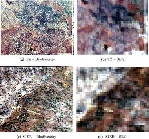
Which allowed the noise to be added to the reflectance images. $L_{\mathrm{a}\mathrm{t}\mathrm{m}\mathrm{o}\mathrm{s}\mathrm{p}\mathrm{h}\mathrm{e}\mathrm{r}\mathrm{e}}$, $E$ and $\tau$ were obtained for each AVIRIS-NG image using the COCHISE (Poutier et al. 2002) in-house atmospheric correction code. Examples of synthetic Biodiversity and SBG images are given in Figure 3. $a$ and $b$ values were given by CNES.

Figure 3. Color compositions of the synthetic hyperspectral images over TZ and SJER for June 2014.

2.4. Radiative transfer modelling and PLS regression

DART 5.7.8v1173 was used for the present study. It is a Monte-Carlo three dimensionnal RTM simulating light interactions and multiple scattering effects within a scene, accounting for topography and atmosphere. A thorough description of the DART model can be found in Sensing, Remote, of Environment, and Toulouse Iii (2016) and Gastellu-Etchegorry et al. (2015). Trees can be defined thanks to various structural parameters such as crown dimensions, location, or the distribution and angular orientation of the foliage. The optical properties of the leaves are obtained with the leaf RTM PROSPECT-D Féret et al. (2017). The good performances of DART as a 3D RTM have been demonstrated consistently in several studies, notably during its participation in the RAMI experiments (Pinty et al. 2001, 2004; Widlowski et al. 2007, 2013).

Trees were modelled within DART with an ellipsoidal crown, following the average proportions of the principal dimensions (width, height, size) of the broad-leaved trees measured on the sites, and distributed along the DART scenes so that the bidirectional reflectance factor (BRF) was the closest to a forest BRF, in a similar fashion as what was done by Gastellu-Etchegorry, Gascon and Estève (2003) and Gascon et al. (2004). The trunk and branches 3D models modelled from the lidar cloud points were imported within DART to represent the non-photosynthetic elements of the trees, as done by Miraglio et al. (2021). Table 3 presents the characteristics of the scenes. DART was used in the Lux mode, with a pixel size of 20 cm and a target ray density per pixel of 200. The spectral bands simulated spanned the 0.5–2.4 μm range, with a 10 nm spatial resolution and a 10 nm FWHM, for a total of 140 spectral bands. The ground was modelled as a flat lambertian surface whose reflectance was set to the average value of pixels selected in the open parts of the AVIRIS-C images through an NDVI criterion: all non-water pixels with a NDVI below 0.3 were considered to correspond to the understory.

Table 3. Values and ranges used to model the forest scenes within the DART model.

Canopy structural parameters	Values & ranges
Canopy Closure (CC)	30; 50; 70; 90%
Crown shape	ellipsoidal
Crown diameter	8.2 m
Crown height	10.4 m
Height below crown	4.1 m
Ground parameters
Type	lambertian surface
Soil reflectance	from AVIRIS-C images
Leaf parameters
Leaf Angle Disitribution (LAD)	ellipsoidal
Average Leaf Angle (ALA)	55 – 65°
Leaf Area Index (LAI)	1–4 m${ }^2$.m${ }^{-2}$
Leaf chlorophylls content (C${ }_{ab}$)	5–70 μg.cm${ }^{-2}$
Leaf carotenoids content (Car)	following the Car/C${ }_{ab}$ relationship
Equivalent Water Thickness (EWT)	0.001–0.025 g.cm${ }^{-2}$
Leaf Mass per Area (LMA)	0.001–0.025 g.cm${ }^{-2}$
Structural parameter (N)	1.5–2.1

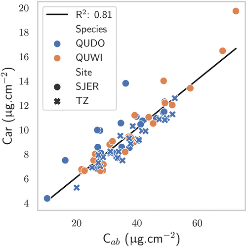
The various CC were obtained by keeping the same tree dimensions and adjusting the scene dimensions and tree positions. The leaf parameter values were randomly picked following a Latin hypercube sampling. In total, 1,600 combinations were generated, to arrive at 400 combinations for each CC. From the lab measurements, it appeared that a relationship could be established between Car and C${ }_{ab}$ contents no matter the site, season and tree species. As such, Car contents were taken within 2.5 standard deviation of the linear relationship presented in Figure 4 to keep simulated cases realistic.

Figure 4. Relationship between Car and C${ }_{ab}$ in SJER and TZ for the two broad-leaved species.

DART allows computing the gap fraction of the forest scenes by setting the atmospheric scattering of sun radiance (SKYL) to 1 and measuring the radiative fraction intercepted by the ground. The resultant gap fraction variation range of the DART outputs was 19–55%, admittedly lower than some in situ measurements. However, as LAI and CC were both already very low, it was decided not to lower them further so as not to confuse the estimator when training on scenes with too little foliage, and instead let the PLSR extrapolate if needed. Finally, all reflectances resulting from the DART simulations were noised using a multiplicative wavelength-independant noise ${\in }_m\sim \mathcal{N}(1,0.02)$.

Different subsets of the 0.5–2.4 μm range were used for each of the vegetation traits, according to their respective contribution to canopy reflectance (Xiao et al. 2014). For gap fraction, the whole range was used; for C${ }_{ab}$ and Car, only bands over the 0.5–0.8 μm; for EWT and LMA, following the findings of Miraglio et al. (2021), bands over the 1.5–2.4 μm range were used in order to limit the influence of the modelling abstractions on estimates accuracy.

PLSR is an estimation method appropriate when model input variables present strong multicollinearities, as they are projected in a new space so that the variance is maximized between the response and the variables. It models a relationship between p variables $\mathbf{X}\in {\mathrm{\Re }}^{n\times p}$ and $l$ outputs $\mathbf{Y}\in {\mathrm{\Re }}^{n\times l}$, with $n$ samples, as per Equation 6,

(6) $\begin{array}{c}\mathbf{X}=\mathbf{T}{\mathbf{P}}^{\mathbf{T}}+\mathbf{E}\\ \mathbf{Y}=\mathbf{T}{\mathbf{Q}}^{\mathbf{T}}+\mathbf{F}\\ \mathbf{T}=\mathbf{X}\mathbf{W}{({\mathbf{P}}^{\mathbf{T}}\mathbf{W})}^{-1}\end{array}$(6)

with $\mathbf{T}\in {\mathrm{\Re }}^{n\times A}$, $\mathbf{P}\in {\mathrm{\Re }}^{A\times p}$, and $\mathbf{E}\in {\mathrm{\Re }}^{n\times p}$ the score, loadings, and residual matrices of $\mathbf{X}$, respectively; $\mathbf{Q}\in {\mathrm{\Re }}^{A\times l}$, and $\mathbf{F}\in {\mathrm{\Re }}^{n\times l}$ are the loadings and residual matrices of $\mathbf{Y}$, respectively; $\mathbf{W}\in {\mathrm{\Re }}^{A\times p}$ is the weight matrix; $A$ is the number of latent variables in the PLSR. While mostly used in chemometrics, it has been successfully applied to remote sensing data on several occasions (Axelsson et al. 2013; Feilhauer, Asner et al. 2015, 2015; Meacham-Hensold et al. 2019).

Before processing, reflectance spectra, gap fraction, C${ }_{ab}$, Car, EWT and LMA were mean-centred and scaled. As Mevik, Segtnan and Næs (2004) showed that bagged PLSR were less sensitive to overfitting, an ensemble of 300 bagged PLSR was used in this study to improve the consistency of the results. For each vegetation trait (gap fraction, C${ }_{ab}$, Car, EWT, LMA), the ensemble was trained on 75% of the databases (hereafter refered to as the training set), the remaining 25% serving as testing set.

The optimal number of latent variables in the PLSR $n_{opt}$ was determined through Monte-Carlo resampling, as described in Kvalheim et al. (2018): the training data was repeatedly divided into calibration and validation sets, and for each set the root-mean-square error (RMSE) obtained over the validation sets was computed for $a$ = 1, 2, … ,$a$ latent variables to define distributions of RMSE for each number of latent variables. The number $A_{min}$ with the lowest median RMSE is identified, and the fraction $A_{min}$ of the RMSE values of $A_{min}$ that exceeded the median RMSE for the preceding latent variables is determined. $A_{min}$ corresponds to a probability measure and can be used to automatically determine if the RMSE with $A_{min}$ latent variables is significantly lower than the RMSE for the preceding number of latent variables ($A_{min}$-1) for a preselected threshold ($A_{min}$). If so, it defines the optimum number of PLS variables as $A_{min}$. If not, $A_{min}$=$A_{min}$-1 and the process is repeated until significance is achieved. For this study, 500 repetitions were made to compute the RMSE distributions, $A_{min}$ was set to 0.401 and the calibration/validation ratio was 50/50.

Hyperspectral data contain multiple variables (i.e. information over several spectral bands), and prediction performance can be improved by a preliminary selection of the relevant variables. Concerning PLSR, a common method, which has been shown to be one of the most consistent by Wang, Peter He and Wang (2015), is to select the variables of interest based on their importance in the projection (variable importance in projection (VIP)). The VIP of the $j^{th}$ variable in a PLSR with $A$ components is scored according to Equation 7,

(7) $\mathrm{V}\mathrm{I}{\mathrm{P}}_j=\sqrt{\frac{p{\mathrm{\Sigma }}_{a=1}^{A}SS(q_a{t}_a){(w_{ja}/||w_a||)}^2}{{\mathrm{\Sigma }}_{a=1}^{A}SS(q_a{t}_a)}}$(7)

with $SS(q_a{t}_a)=q_a^2{t}_a^T{t}_a$; $t_a$ the $a^{th}$ column vector of $\mathbf{T}$; $q_a$ the $a^{th}$ element of the regression vector $q$ of $\mathbf{T}$; $w_a$ is the $a^{th}$ column vector of $\mathbf{W}$; $p$ the number of variables in $\mathbf{X}$. Once the VIP scores have been obtained for each variable, only variables with a score greater than one are retained and the others are deemed as not significant.

For each variable (gap fraction, C${ }_{ab}$, Car, EWT, LMA) and each hyperspectral image, one bagged PLSR model was trained.

2.5. PLSR application and estimates accuracy assessment

Once trained, the bagged PLSR were used to estimate C${ }_{ab}$, Car, EWT, LMA, and, when possible, gap fraction from the AVIRIS-C, SBG, and Biodiversity images, providing estimation maps.

As the GSD of SBG is quite large with regards to the CC of the sites, estimated accuracy was first assessed by comparing the traits’ values measured in situ to the values estimated in the pixels closest to the GPS positions for both AVIRIS-C and SBG and evaluating the RMSE and R${ }^2$. Using the CC maps derived from the AVIRIS-NG images (Miraglio et al. 2019), pixels could be distinguished by the values of the underlying canopy, potentially allowing identification of behaviours depending on its closure. The AVIRIS-C estimation map was spatially resampled to 30 m with a 30 m FWHM averaging filter in order to study the coherency of AVIRIS-C and SBG estimates. For each date, RMSE and R${ }^2$ between AVIRIS-C and SBG estimations were computed, a low RMSE and high R${ }^2$ indicating good consistency of the estimations across sensors.

Concerning Biodiversity data, only one date was available for each site, greatly reducing the number of validation points. Still, in situ measurements were once again compared to the pixels of the estimate map. Only C${ }_{ab}$ and Car were estimated, as no field data equivalent to a tree gap fraction was available. To complete the accuracy assessment and overcome the small quantity of validation points, the Biodiversity images were, in a similar fashion as in the previous subsection, spatially resampled to 30 m to compare estimates of behaviours across CC and cross-validate the estimated values.

3. Results

3.1. Canopy cover within the sensors’ pixels

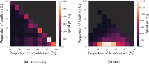
The canopy cover within Biodiversity and SBG pixels was assessed using tree-type classification maps that had been obtained in previous works (Miraglio et al. 2021). Figure 5 shows the pixel canopy composition of the Biodiversity and SBG images of TZ, derived from one of the classification maps. Unsurprisingly, it appears that the vegetation pixels of Biodiversity contain a high proportion of vegetation. Most of the time, the canopy cover of vegetation pixels is around 100%, with a preponderance of QUDO: from the histogram, it appears that QUDO crowns represent 85, 95, and 65% of pixels’ contents from the three most common categories. Overall, most vegetation pixels of the Biodiversity image are on the diagonal, i.e. have almost 100% CC. Comparatively, most vegetation pixels in the SBG image only had a CC of about 50%, a result consistent with the field measurements presented in Section 2.1.1.

Figure 5. Histograms of the CC of conifers and broad-leaved trees of TZ within the pixels of the hyperspectral images.

3.2. DART-Generated spectral databases

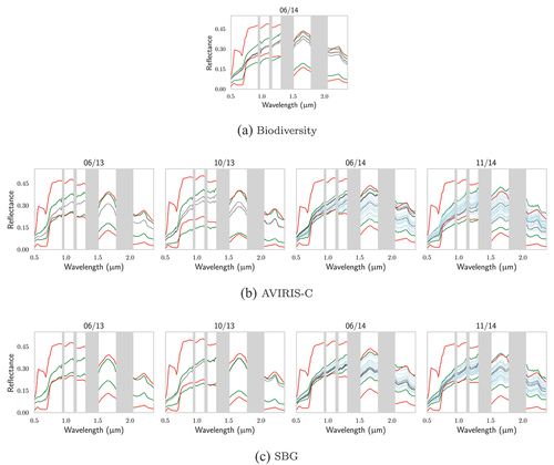
First, the databases generated with DART to train the PLSR were compared to the AVIRIS-C, SBG and Biodiversity hyperspectral images to assess their adequacy to retrieve vegetation traits. Vegetation pixels within the image were identified by looking for pixels whose NDVI was above that of the reflectance used to model the understory within the DART model. In Appendix A, Figures A1 and A2 illustrate how well the databases encompass the hyperspectral images’ vegetation reflectances. Concerning TZ, almost all vegetation pixels were within the databases boundaries over the whole spectral range for both AVIRIS-C and SBG. Only some pixel reflectances were below the database values around 0.8 μm, giving confidence in the ability of PLSR trained from these databases to yield accurate predictions. For SJER, the results were not as good, with a recurrent overestimation of the reflectance in over the 0.8–1.5 μm range, especially visible for the two images acquired during the fall (10/13 and 11/14). Moreover, it appears that some pixels that correspond to in situ measurements are not detected as vegetation pixels: for SJER images corresponding to 06/13 and 10/13, from AVIRIS-C to SBG, some spectra disappear as the pixel’s NDVI becomes too low. For the two Biodiversity images, not all vegetation pixels were within the databases’ boundaries. It appears that for both SJER and TZ, some pixel reflectances may be lower than those of the databases over the 0.8–1.5 μm region. Moreover, concerning TZ, some reflectances were also above those of the database over the 1.5–2.4 μm region. Overall, 71% of the vegetation pixels were completely within database boundaries for the Biodiversity image of TZ, while it was 55% for SJER.

3.3. Bagged PLSR predictions over the hyperspectral images

Table 4 presents the main statistics of the bagged PLSR models after their fit on the synthetic datasets from each date. Concerning the training datasets, RMSE and R${ }^2$ values are consistent across sites and dates, with similar values for each vegetation trait. RMSE are about 0.03, 8.5 μg.cm${ }^{-2}$, 1.5 μg.cm${ }^{-2}$, 0.0035 g.cm${ }^{-2}$ and 0.004 g.cm${ }^{-2}$ for gap fraction, C${ }_{ab}$, Car, EWT, and LMA, respectively. Goodness of fit is high (R${ }^2$ $\ge$ 0.69) for every case. Over the test sets, performances remained similar, with little change to both RMSE and R${ }^2$ values.

Table 4. Statistics of the bagged PLSR models when predicting the vegetation traits over the train and test databases and over the hyperspectral images.

		Gap fraction			C${ }_{ab}$			Car			EWT			LMA
						RMSE			RMSE			RMSE			RMSE
	MM/YY	$n_{opt}$	RMSE	R${ }^2$	$n_{opt}$	(μg.cm${ }^{-2}$)	R${ }^2$	$n_{opt}$	(μg.cm${ }^{-2}$)	R${ }^2$	$n_{opt}$	(g.cm${ }^{-2}$)	R${ }^2$	$n_{opt}$	(g.cm${ }^{-2}$)	R${ }^2$
Train
TZ	06/13				6	8.79	0.78	6	1.55	0.77	4	0.0036	0.74	4	0.004	0.69
	09/13				6	9.21	0.76	6	1.62	0.75	4	0.0036	0.74	4	0.0039	0.71
	06/14	7	0.03	0.96	6	8.5	0.79	7	1.55	0.77	4	0.0034	0.76	2	0.0038	0.72
SJER	06/13				4	8.71	0.78	4	1.55	0.77	4	0.0035	0.76	4	0.0037	0.73
	10/13				6	8.66	0.79	6	1.48	0.79	4	0.0035	0.75	4	0.0036	0.74
	06/14	6	0.03	0.95	4	8.54	0.79	4	1.59	0.76	4	0.0035	0.76	4	0.0036	0.74
	11/14	7	0.02	0.97	6	8.91	0.77	6	1.54	0.78	4	0.0036	0.74	4	0.0038	0.72
Test
TZ	06/13					8.77	0.79		1.54	0.79		0.0035	0.75		0.0039	0.71
	09/13					9.47	0.76		1.61	0.78		0.0036	0.74		0.0041	0.69
	06/14		0.03	0.95		8.67	0.8		1.51	0.8		0.0035	0.76		0.0036	0.75
SJER	06/13					8.81	0.79		1.55	0.8		0.0035	0.75		0.0038	0.73
	10/13					9	0.79		1.47	0.82		0.0035	0.75		0.0036	0.76
	06/14		0.03	0.94		9.07	0.78		1.58	0.79		0.0036	0.74		0.0035	0.77
	11/14		0.02	0.96		8.9	0.79		1.49	0.81		0.0038	0.72		0.0038	0.72
Application (all dates)
Biodiversity						8.5	0.03		2.24	0.18		0.0071	0.11		0.0049	0.61
AVIRIC-C			0.09	0.8		7.91	0.26		1.73	0.05		0.0079	0.		0.0053	0.07
SBG			0.1	0.59		7.44	0.33		1.6	0.17		0.004	0.11		0.0035	0.2

For the hyperspectral images, predictions for all dates were pooled together to compute the statistics. Estimated accuracy for C${ }_{ab}$ and Car remained similar to what was obtained over the synthetic databases (RMSE are about 8 and 1.75 μg.cm${ }^{-2}$, respectively) for all sensors. Gap fraction was also well estimated with a RMSE of 0.1, higher than in the testing phase, and R${ }^2$ values of 0.8 and 0.59 for AVIRIS-C and SBG, respectively. EWT and LMA estimations over the hyperspectral images were quite poor: ignoring results for Biodiversity, which only had seven in situ points to compute the statistics, R${ }^2$ were always very low and no relation between estimates and field measurements were found. RMSE values for EWT and LMA are similar for Biodiversity and AVIRIS-C (undefined.0075 and undefined.0050 g.cm${ }^{-2}$ for EWT and LMA, respectively), but appeared to be lower for SBG (0.004 and 0.0035 g.cm${ }^{-2}$).

3.4. Impact of the GSD on estimates

As visible in Figure 6, gap fraction was well estimated no matter the CC of the hyperspectral pixels for both AVIRIS-C and SBG. Concerning C${ }_{ab}$ and Car estimation, and especially for AVIRIS-C, it appeared that high-CC pixels (CC $\ge$ 90%) led to more accurate estimations than those with lower CC. Overall, estimates were coherent between AVIRIS-C and SBG. Table 5 shows the results of the comparison of these estimates, considering not only RMSE and R${ }^2$ but also systematic and unsystematic RMSE (RMSE${ }_s$ and RMSE${ }_u$, respectively (Willmott 1981)) over different CC (low, around 40%, and high, above 80%). For all vegetation traits, coherency was only slightly improved going from the low to the high CC areas, and a good fit was always obtained (R${ }^2>$ 0.3 for gap fraction and C${ }_{ab}$, and R${ }^2>$ 0.5 for other traits). After AVIRIS-C estimates were aggregated to 30 m, RMSE between AVIRIS-C and SBG C${ }_{ab}$, EWT and LMA values were lower than those obtained when comparing the estimates with in situ measurements. For gap fraction and Car, these RMSE values were of the same order.

Figure 6. Comparison between vegetation traits as estimated by the PLSR and the in situ measurements for the AVIRIS-C images: gap fraction, C${ }_{ab}$, Car, EWT, LMA. The hue of the markers depends on the CC of the hyperspectral pixels that were considered. Black markers correspond to zones where CC information was not available.

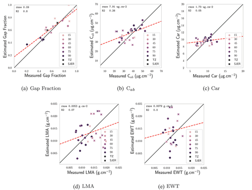
Table 5. Comparison between the values estimated from different sensors over two CC zones of TZ.

	30% $\le$ CC $\le$ 50%					80% $\le$ CC
		Cab	Car	EWT	LMA		Cab	Car	EWT	LMA
	Gap frac.	μg.cm${ }^{-2}$	μg.cm${ }^{-2}$	g.cm${ }^{-2}$	g.cm${ }^{-2}$	Gap frac.	μg.cm${ }^{-2}$	μg.cm${ }^{-2}$	g.cm${ }^{-2}$	g.cm${ }^{-2}$
Comparison between SBG and AVIRIS-C estimates
RMSE	0.1	2.86	2.4	0.0034	0.0021	0.12	3.65	3.22	0.0030	0.0021
RMSE${ }_s$	0.09	2.21	2.3	0.0009	0.0001	0.11	3.24	3.17	0.0001	0.0004
RMSE${ }_u$	0.1	1.81	0.66	0.0034	0.0021	0.05	1.69	0.52	0.0030	0.002
R${ }^2$	0.35	0.34	0.52	0.5	0.55	0.42	0.52	0.66	0.59	0.6
Comparison between SBG and Biodiversity estimates
RMSE		5.59	1.38	0.0079	0.0052		3.56	1.43	0.0065	0.0059
RMSE${ }_s$		0.65	0.64	0.0069	0.0042		0.36	1.19	0.0057	0.0054
RMSE${ }_u$		5.55	1.23	0.0079	0.0052		3.54	0.85	0.0031	0.0022
R${ }^2$		0.2	0.07	0.2	0.25		0.48	0.39	0.29	0.32

However, the predictions from SBG and Biodiversity imagery could be significantly dissimilar. Two different behaviours are visible for C${ }_{ab}$ and Car estimations between the low and high CC zones. While the most significant change happened for C${ }_{ab}$, whose RMSE was improved from 5.59 to 3.56 μg.cm${ }^{-2}$ from one CC category to the other, estimates for all vegetation traits (C${ }_{ab}$, Car, EWT, LMA) presented a clearly lower RMSE${ }_u$ between Biodiversity and SBG over the closed parts of the canopy than the open parts. It appears that over closed canopies estimates from Biodiversity and SBG images were well correlated (0.48 $\ge$ R${ }^2$ $\ge$ 0.32), even though a constant bias could be present for some traits. This was not the case over the open parts (CC $\sim$ 40%) where no relationship could be found between SBG and Biodiversity estimates. In particular for C${ }_{ab}$, R${ }^2$ was only 0.2 with a large dispersion of the points around 40 μg.cm${ }^{-2}$.

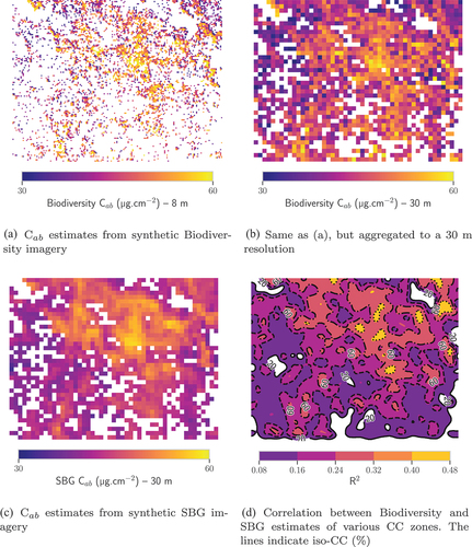
Finally, to complement the results presented in Table 5, Figure 7 shows the correlation between C${ }_{ab}$ estimations from Biodiversity and SBG over TZ for June 2014. The estimation map from Biodiversity was spatially averaged to attain a 30 m resolution and allow comparison with the SBG-derived map. For the CC categories 20–40%, 40–60%, 60–80% and 80–100%, the R${ }^2$ between Biodiversity and SBG estimates were computed. As visible in Figure 7, the lower the CC, the lower the correlation. For the savanna portion of TZ, with a CC $\le$ 60%, the R${ }^2$ is lower than 0.24. Estimates from the sensors are mostly in agreement over the CC $\ge$ 80% areas (with a R${ }^2$ of 0.48), that are spatially very limited.

Figure 7. Comparison between C${ }_{ab}$ estimates from Biodiversity and SBG imagery over TZ. Pixels whose NDVI was lower than those that could be computed from the spectra of the training databases were masked.

4. Discussion

4.1. Adequacy of the training databases to the hyperspectral images

As visible in Figures A1 and A2, over parts of the 0.5–2.4 μm range the vegetation reflectance was not within the boundaries of the synthetic databases, especially over the 0.8–1.5 μm range. As showed by Miraglio et al. (2021), this may partly be due to the lack of detail in the modelling of the trees within DART. The findings were in agreement with the results of Widlowski, François Côté and Béland (2014) who showed that, in both the red and near-infrared (NIR) regions, a simplified forest representation could lead to high biases ($>$ 10%) for the spatial resolutions considered in the present study. Moreover, Malenovský et al. (2008) demonstrated that introducing small woody components in the DART tree crowns would lead to lower reflectance in the NIR. As a consequence the present study only focused on the 1.5–2.4 μm spectral interval to for EWT and LMA retrieval. In a more general manner, the present study considered an ellipsoidal LAD with a free ALA varying from 55° to 65°, broadly encompassing the spherical and erectophil LAD. Indeed, from 1200 leaf inclination measurements, Ryu et al. (2010) had found that, in summer, TZ tree leaves presented an ALA of 62° and an erectophil LAD. Erectophilic leaves have indeed been observed in arid environments, and are associated with drought-tolerance adaptation to reduce midday heating and maximize the photosynthetic activity during morning and evening, when the leaf water potential is highest (Crawford and Gibson 1997). However, LAD may vary spatially and temporally, and these results may not be applicable to other seasons and sites. A spherical LAD is often assumed in the absence of in situ measurements (Bonan et al. 2011; Ryu et al. 2011). This assumption is questionable: both Pisek et al. (2013) and Liu et al. (2019) found, for temperate broad-leaved forests, that planophil or plagiophil distributions, whose ALA are closer to 30° and 45°, respectively (Chianucci et al. 2018), were more representative of the LAD of mature stands and may be more adequate for modelling purposes.

Another possible limitation in the DART modelling was that the ground reflectance was directly set as the average of understory pixels from the hyperspectral image. This was done as it was one of the most simple and straightforward methods, easily implementable in an operational context. However, within-site variability of ground reflectance was not taken into account, and the database was built considering only the median value of the pure ground pixels identified within the images. Bach and Verhoef (2003) and Darvishzadeh et al. (2008) showed that soil backgrounds strongly affected canopy reflectance, especially at low LAI. The acquisitions in the present study always took place during dry days, limiting the effects of soil moisture affecting the reflected variation. However, Eriksson et al. (2006) demonstrated that the understory vegetation had a significant effect on the red and NIR spectral ranges: spatial heterogeneity of the understory could have led to inadequacies of the SJER databases for some parts of the site, as SJER canopies are considerably more open than TZ on average (30% and 50%, respectively).

A solution to improve the adequacy of the synthetic databases for inversion purposes could be either to take into account the heterogeneity of the ground reflectance, by making it a free-varying parameter, or to build one database per ground reflectance and use the more adequate one based on the spatial information from the image. The first solution, while in theory leading to very generalizable databases, may lead to suboptimal fits when training machine-learning methods, but could be employed regardless the GSD of the sensor that acquired the images. The second method would require a high spatial resolution to clearly distinguish the ground surrounding the tree crowns and choose the best-corresponding database: while not realistic for SBG, this could be done with images acquired with sensors with a finer spatial resolution such as Biodiversity.

4.2. Vegetation trait estimates from airborne and satellite hyperspectral imagery

The results displayed in Figure 6 showed that, for the more closed parts of the canopy, a PLSR fit on synthetic data was able to retrieve C${ }_{ab}$ and Car with high accuracy. While the dispersion was greater in the open parts, RMSE remained low overall when considering the whole dataset, and the PLSR estimates remained close to the in situ values. Moreover, gap fraction estimates are good no matter the CC and, evidently, related to it: it is therefore possible to get an idea of the estimates’ accuracy by assessing their respective gap fractions. The good results for gap fraction are particularly encouraging, as specified in Section 2.4.4, the gap fraction variation range was only 19–55% in the training database: values outside of this range were also well predicted. Overall, estimated gap fraction, C${ }_{ab}$ and Car values were in line with what was obtained in Miraglio et al. (2020) and in previous studies. In Miraglio et al. (2020), a LUT-based inversion with less variable parameters had been used, reducing the possible generalization of the method, and being more time-consuming in the inversion phase. The accuracy obtained here for gap fraction estimates (RMSE: 0.09; R${ }^2$: 0.8) was in line with what had obtained Baret, Clevers and Steven (1995) when using a neural network trained with synthetic data over crop fields (RMSE: 0.09; R${ }^2$: 0.9). The present study shows that equivalent accuracies are attainable with a PLSR trained on more general synthetic data.

Similar performances were obtained with the SBG hyperspectral images. As indicated in Table 4, it seems that C${ }_{ab}$, Car, EWT, and LMA estimates are all improved with this GSD, as all RMSE values are lower when comparing estimated values with in situ measurements. However, it appears that AVIRIS-C and SBG images are overall equivalent when it comes to estimations over TZ, as shown in Table 5. The slightly coarser spatial resolution (30 m instead of 18 m) does not seem to affect much retrieval accuracy, which is encouraging: results obtained with, and methods developed for, AVIRIS-C images may be directly transportable to SBG.

Over the high-CC areas, Biodiversity and SBG images led to similar C${ }_{ab}$ and Car estimation. For those areas the influence of understory reflectance is minimal (CC $\ge$ 80%), and as discussed above estimate accuracy from the SBG images was good. This correlation between Biodiversity and SBG estimations further confirms that acceptable retrieval is possible from Biodiversity images, despite its lower SNR. Moreover, as shown in Figure 5, the majority of vegetation pixels in the Biodiversity images have CC higher than 80%: Biodiversity is barely affected by the openness of canopies as tree crowns can be, most of the time, isolated. Thus, the lack of relationship between Biodiversity and SBG estimates for low-CC zones is illustrative of the advantage of a finer spatial resolution for mapping vegetation traits over open canopies. These results are consistent with what Carter et al. (2009) and Jafari and Lewis (2012) found: the spatial resolution of the hyperspectral images is a limiting factor, especially for open canopies: identifying spectrally pure pixels used for estimation or classification purposes is all the more difficult. Heldens et al. (2011) suggested to use data fusion to make EnMAP acquisitions fit for use in an urban context, as their original resolution would not allow to distinguish the various objects. In a similar vein, Siegmann et al. (2015) showed the potential of pan-sharpening for improving LAI retrieval accuracy of wheat fields when working with EnMAP images. The high spatial resolution of Biodiversity could therefore prove useful either for direct use in the retrieval of vegetation traits, or indirectly through data fusion with images acquired by other sensors. More recently, working with Sentinel-2A images, Zarco-Tejada et al. (2019) have shown that being able to account for the specificities of each pixel components was critical to obtain acceptable C${ }_{ab}$ estimations over sparse canopies. Overall, there seems to be a clear potential in taking advantage of the smaller GSD of Biodiversity to improve vegetation traits’ retrieval, either directly from the sensor’s acquisitions or indirectly through data fusion, despite its lower expected SNR.

The present study did not have the in situ measurements to directly map LAI from either the SBG or Biodiversity images. While performances for the gap fraction estimations using SBG images hint at potentially good accuracy for LAI, this would necessitate further works to confirm. Validation of Biodiversity LAI estimates would require the field measurement of isolated trees’ LAI, possibly requiring lidar measurements to obtain these values (Klingberg et al. 2015; Béland et al. 2014).

No clear conclusion can yet be drawn for EWT and LMA: for the high-CC areas, the variation range of the in situ measurements is rather limited, so that it is not possible to say whether or not estimations from the SBG image are really accurate. However, it must be noted from Table 5 that EWT and LMA estimates from the high-CC areas are similar between Biodiversity and SBG. While RMSE is high, it is mostly due to a systematic bias, and the unsystematic RMSE is only 0.0022 g.cm${ }^{-2}$ for both EWT and LMA, while the variation range is roughly 0.007–0.023 g.cm${ }^{-2}$. That estimations from hyperspectral images with so different spatial resolutions show similar behaviours may indicate that, while some bias is present, EWT and LMA can be retrieved from SBG images for closed canopies and a fortiori from Biodiversity images.

5. Conclusion

This study assessed the potential of the future hyperspectral missions SBG (30 m GSD) and Biodiversity (8 m GSD) for the mapping of vegetation traits (gap fraction, C${ }_{ab}$, Car, EWT, LMA) of broad-leaved trees in two woodland savannas in California, using synthetic data generated from AVIRIS-NG and AVIRIS-C images. The accuracy of the traits’ estimates from a hybrid method, using a PLSR trained on DART-generated data, was assessed through (i) direct comparison with in situ measurements and (ii) intercomparison between the values obtained from AVIRIS-C, Biodiversity, and SBG images. SBG and AVIRIS-C gap fraction, C${ }_{ab}$, and Car estimates showed great correspondence with ground-based values (RMSE $\sim$ 0.1, R${ }^2$ $\sim$ 0.65; RMSE $\sim$ 7.7 μg.cm${ }^{-2}$, R${ }^2$ $\sim$ 0.3; RMSE $\sim$ 1.7 μg.cm${ }^{-2}$, R${ }^2$ $\sim$ 0.1, respectively), however concerning pigments this was more true for the densest parts of the canopy. At the landscape scale, there was in general sufficient agreement at 30 m GSD between retrievals from SBG and AVIRIS-C imagery for all traits (R${ }^2$ ranging from 0.34 to 0.66). Biodiversity estimates were also consistent with SBG estimates over the closed parts of the canopy (R${ }^2$ ranging from 0.32 to 0.48), giving confidence in the accuracy of the estimates, but exhibited different behaviours over the open parts, probably owing to increased spectral mixing in the SBG pixels affecting the estimation.

This work not only demonstrates that gap fraction, C${ }_{ab}$ and Car estimations are possible using 30 m GSD satellite data over the more closed parts of canopies without detailed information concerning the imaged landscape, but also shows the potential of $\sim$ 8 m GSD images to map the five vegetation traits considered in this study over any canopy. Despite their lower SNR, hyperspectral satellite sensors with finer spatial resolution could prove very beneficial to the global mapping of vegetation traits by complementing sensors with coarser GSD when working over highly heterogeneous canopies. Finally, this study found that training a PLSR model over synthetic data led to acceptable estimates accuracy over images that would be acquired by hyperspectral satellite sensors. Such hybrid methods are therefore very promising in the context of the recently launched PRISMA and EnMAP missions.

Acknowledgements

The authors are grateful to the John Muir Institute of the Environment team for collecting and processing the field data, and to NASA JPL from providing AVIRIS-C data (NASA grant No. NNX12AP08G). They also thank Jean-Philippe Gastellu-Etchegorry from CESBIO for his insight and help concerning the DART simulations.

Disclosure statement

The authors declare no conflict of interest. The funders had no role in the design of the study; in the collection, analyses, or interpretation of data; in the writing of the manuscript, or in the decision to publish the results.

Data availability statement

The data that support the findings of this study are available on request from the corresponding author, T.M. The data are not publicly available due to company policy.

Correction Statement

This article has been corrected with minor changes. These changes do not impact the academic content of the article.

Additional information

Funding

This research was funded by the Office Nationale d’Études et de Recherches Aérospatiales (ONERA) and by Région Occitanie.

Appendix.

Suitability of DART-generated databases

Figure A1. For TZ, comparison of (in red) the extrema of the DART-generated databases for Biodiversity, AVIRIS-C and SBG with: (in green) the extrema of the vegetation pixels of their respective images; the reflectances of the pixels associated with in situ (in black) biochemistry and (in blue) gap fraction measurements.

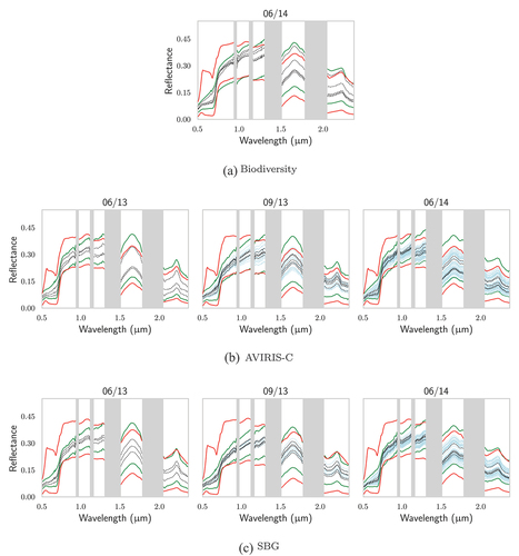
Figure A2. For SJER, comparison of (in red) the extrema of the DART-generated databases for Biodiversity, AVIRIS-C and SBG with: (in green) the extrema of the vegetation pixels of their respective images; the reflectances of the pixels associated with in situ (in black) biochemistry and (in blue) gap fraction measurements.

References

- Ali, A. M., R. Darvishzadeh, A. Skidmore, T. W. Gara, and M. Heurich. 2020. “Machine Learning Methods’ Performance in Radiative Transfer Model Inversion to Retrieve Plant Traits from Sentinel-2 Data of a Mixed Mountain Forest.” International Journal of Digital Earth 14 (1): 106–120.
- Asner, G. P., R. E. Martin, C. B. Anderson, and D. E. Knapp. 2015. “Quantifying Forest Canopy Traits: Imaging Spectroscopy versus Field Survey.” Remote Sensing of Environment 158: 15–27. doi:10.1016/j.rse.2014.11.011.
- Axelsson, C., A. K. Skidmore, M. Schlerf, A. Fauzi, and W. Verhoef. 2013. “Hyperspectral Analysis of Mangrove Foliar Chemistry Using PLSR and Support Vector Regression.” International Journal of Remote Sensing 34 (5): 1724–1743. doi:10.1080/01431161.2012.725958.
- Bach, H. and W. Verhoef. 2003. “Sensitivity Studies on the Effect of Surface Soil Moisture on Canopy Reflectance Using the Radiative Transfer Model geoSail.” In International Geoscience and Remote Sensing Symposium (IGARSS) Toulouse, Vol. 3, 1679–1681. IEEE.
- Baret, F., J. G. P. W. Clevers, and M. D. Steven. 1995. “The Robustness of Canopy Gap Fraction Estimates from Red and Near-Infrared Reflectances: A Comparison of Approaches.” Remote Sensing of Environment 54 (2): 141–151. doi:10.1016/0034-4257(95)00136-O.
- Béland, M., D. D. Baldocchi, J. Luc Widlowski, R. A. Fournier, and M. M. Verstraete. 2014. “On Seeing the Wood from the Leaves and the Role of Voxel Size in Determining Leaf Area Distribution of Forests with Terrestrial LiDar.” Agricultural and Forest Meteorology 184: 82–97. doi:10.1016/j.agrformet.2013.09.005.
- Berger, K., C. Atzberger, M. Danner, G. D’-Urso, W. Mauser, F. Vuolo, and T. Hank. January 2018. “Evaluation of the PROSAIL Model Capabilities for Future Hyperspectral Model Environments: A Review Study.” Remote Sensing 10 (2): 85. doi:10.3390/rs10010085.
- Bonan, G. B., P. J. Lawrence, K. W. Oleson, S. Levis, M. Jung, M. Reichstein, D. M. Lawrence, and S. C. Swenson. 2011. “Improving Canopy Processes in the Community Land Model Version 4 (CLM4) Using Global Flux Fields Empirically Inferred from FLUXNET Data.” Journal of Geophysical Research 116 (G2). doi:10.1029/2010JG001593.
- Carrere, V., X. Briottet, S. Jacquemoud, R. Marion, A. Bourguignon, M. Chami, and M. Dumont, et al. June 2013. “HYPXIM: A Second Generation High Spatial Resolution Hyperspectral Satellite for Dual Applications.” In Workshop on Hyperspectral Image and Signal Processing, Evolution in Remote Sensing Gainesville, Vol. 2013. IEEE Computer Society.
- Carter, G. A., K. L. Lucas, G. A. Blossom, C. L. L. Holiday, D. S. Mooneyhan, D. R. Fastring, T. R. Holcombe, and J. A. Griffith. 2009. “Remote Sensing and Mapping of Tamarisk Along the Colorado River, USA: A Comparative Use of Summer-Acquired Hyperion, Thematic Mapper and Quickbird Data.” Remote Sensing 1 (3): 318–329. doi:10.3390/rs1030318.
- Chen, Q., D. Baldocchi, P. Gong, and T. Dawson. 2008. “Modeling Radiation and Photosynthesis of a Heterogeneous Savanna Woodland Landscape with a Hierarchy of Model Complexities.” Agricultural and Forest Meteorology 148 (6–7): 1005–1020. doi:10.1016/j.agrformet.2008.01.020.
- Chianucci, F., J. Pisek, K. Raabe, L. Marchino, C. Ferrara, and P. Corona. 2018. “A Dataset of Leaf Inclination Angles for Temperate and Boreal Broadleaf Woody Species.” Annals of Forest Science 75 (2): 50. doi:10.1007/s13595-018-0730-x.
- Cowling, R. M., P. W. Rundel, B. B. Lamont, M. Kalin Arroyo, and M. Arianoutsou. 1996. “Plant Diversity in Mediterranean-Climate Regions.” Trends in Ecology & Evolution 11 (9): 362–366. doi:10.1016/0169-5347(96)10044-6.
- Crawford, R. M. M. and A. C. Gibson. 1997. “Structure-Function Relations of Warm Desert Plants.” The Journal of Ecology 85 (5): 735. doi:10.2307/2960545.
- Dana Chadwick, K. and P. A. Gregory. 2016. “Organismic-Scale Remote Sensing of Canopy Foliar Traits in Lowland Tropical Forests.” Remote Sensing 8 (2): 27.
- Darvishzadeh, R., A. Skidmore, C. Atzberger, and S. van Wieren. 2008. “Estimation of Vegetation LAI from Hyperspectral Reflectance Data: Effects of Soil Type and Plant Architecture.” International Journal of Applied Earth Observation and Geoinformation 10 (3): 358–373. doi:10.1016/j.jag.2008.02.005.
- Darvishzadeh, R., A. Skidmore, H. Abdullah, E. Cherenet, A. Ali, T. Wang, W. Nieuwenhuis, et al. 2019. ”Mapping Leaf Chlorophyll Content from Sentinel-2 and RapidEye Data in Spruce Stands Using the Invertible Forest Reflectance Model.” International Journal of Applied Earth Observation and Geoinformation 79: 58–70. 10.1016/j.jag.2019.03.003.
- Eriksson, H. M., L. Eklundh, A. Kuusk, and T. Nilson. 2006. “Impact of Understory Vegetation on Forest Canopy Reflectance and Remotely Sensed LAI Estimates.” Remote Sensing of Environment 103 (4): 408–418. doi:10.1016/j.rse.2006.04.005.
- Feilhauer, H., G. P. Asner, and R. E. Martin. 2015. “Multi-Method Ensemble Selection of Spectral Bands Related to Leaf Biochemistry.” Remote Sensing of Environment 164: 57–65. doi:10.1016/j.rse.2015.03.033.
- Feingersh, T. and E. Ben Dor. 2015. “SHALOM - a Commercial Hyperspectral Space Mission.” In Optical Payloads for Space Missions, 247–263. Chichester, UK: John Wiley & Sons, Ltd. doi:10.1002/9781118945179.ch11.
- Féret, J. B., A. A. Gitelson, S. D. Noble, and S. Jacquemoud. 2017. “PROSPECT-D: Towards Modeling Leaf Optical Properties Through a Complete Lifecycle.” Remote Sensing of Environment 193: 204–215. doi:10.1016/j.rse.2017.03.004.
- Gao, B.-C. and A. F. H. Goetz. 1990. “Column Atmospheric Water Vapor and Vegetation Liquid Water Retrievals from Airborne Imaging Spectrometer Data.” Journal of Geophysical Research 95 (D4): 3549–3564. doi:10.1029/JD095iD04p03549.
- Gascon, F., J. P. Gastellu-Etchegorry, M. J. Lefevre-Fonollosa, and E. Dufrene. 2004. “Retrieval of Forest Biophysical Variables by Inverting a 3-D Radiative Transfer Model and Using High and Very High Resolution Imagery.” International Journal of Remote Sensing 25 (24): 5601–5616. doi:10.1080/01431160412331291305.
- Gastellu-Etchegorry, J. P., F. Gascon, and P. Estève. 2003. “An Interpolation Procedure for Generalizing a Look-Up Table Inversion Method.” Remote Sensing of Environment 87 (1): 55–71. doi:10.1016/S0034-4257(03)00146-9.
- Gastellu-Etchegorry, J. P., T. Yin, N. Lauret, T. Cajgfinger, T. Gregoire, E. Grau, J. Baptiste Feret, et al. 2015. ”Discrete Anisotropic Radiative Transfer (DART 5) for Modeling Airborne and Satellite Spectroradiometer and LIDAR Acquisitions of Natural and Urban Landscapes.” Remote Sensing 7 (2): 1667–1701. DOI:10.3390/rs70201667.
- Gauquelin, T., G. Michon, R. Joffre, R. Duponnois, D. Génin, B. Fady, M. Bou Dagher-Kharrat, et al. 2018. ”Mediterranean Forests, Land Use and Climate Change: A Social-Ecological Perspective.” Regional Environmental Change 18 (3): 623–636. DOI:10.1007/s10113-016-0994-3.
- Green, R. O., M. L. Eastwood, C. M. Sarture, T. G. Chrien, M. Aronsson, B. J. Chippendale, J. A. Faust, et al. 1998. ”Imaging Spectroscopy and the Airborne Visible/infrared Imaging Spectrometer (AVIRIS).” Remote Sensing of Environment 65 (3): 227–248. DOI:10.1016/S0034-4257(98)00064-9.
- Guanter, L., H. Kaufmann, K. Segl, S. Foerster, C. Rogass, S. Chabrillat, T. Kuester, et al. 2015. ”The EnMap Spaceborne Imaging Spectroscopy Mission for Earth Observation.” Remote Sensing 7 (7): 8830–8857. DOI:10.3390/rs70708830.
- Heldens, W., U. Heiden, T. Esch, E. Stein, and A. Müller. september 2011. “Can the Future EnMap Mission Contribute to Urban Applications? a Literature Survey.” Remote Sensing 3 (9): 1817–1846. doi:10.3390/rs3091817.
- Jafari, R. and M. M. Lewis. 2012. “Arid Land Characterisation with EO-1 Hyperion Hyperspectral Data.” International Journal of Applied Earth Observation and Geoinformation 19 (1): 298–307. doi:10.1016/j.jag.2012.06.001.
- Klingberg, J., J. Konarska, F. Lindberg, and S. Thorsson. 2015. “Measured and Modelled Leaf Area of Urban Woodlands, Parks and Trees in Gothenburg, Sweden.” In ICUC9 - 9th International Conference on Urban Climate jointly with 12th Symposium on the Urban Environment Toulouse, 1–6.
- Kobayashi, H., Y. Ryu, D. D. Baldocchi, J. M. Welles, and J. M. Norman. 2013. “On the Correct Estimation of Gap Fraction: How to Remove Scattered Radiation in Gap Fraction Measurements?” Agricultural and Forest Meteorology 174-175: 170–183. doi:10.1016/j.agrformet.2013.02.013.
- Kvalheim, O. M., R. Arneberg, B. Grung, and T. Rajalahti. 2018. “Determination of Optimum Number of Components in Partial Least Squares Regression from Distributions of the Root-Mean-Squared Error Obtained by Monte Carlo Resampling.” Journal of Chemometrics 32 (4): e2993. doi:10.1002/cem.2993.
- Lee, C. M., M. L. Cable, S. J. Hook, R. O. Green, S. L. Ustin, D. J. Mandl, and E. M. Middleton. 2015. “An Introduction to the NASA Hyperspectral InfraRed Imager (HyspIri) Mission and Preparatory Activities.” Remote Sensing of Environment 167: 6–19. doi:10.1016/j.rse.2015.06.012.
- Lichtenthaler, H. K. 1987. “Chlorophylls and Carotenoids: Pigments of Photosynthetic Biomembranes.” Methods in Enzymology 148 (C): 350–382.
- Lichtenthaler, H. K. and C. Buschmann. 2001. “Chlorophylls and Carotenoids: Measurement and Characterization by UV-VIS Spectroscopy.” Current Protocols in Food Analytical Chemistry 1 (1): F4.3.1–F4.3.8. doi:10.1002/0471142913.faf0403s01.
- Liu, J., A. K. Skidmore, T. Wang, X. Zhu, J. Premier, M. Heurich, B. Beudert, and S. Jones. 2019. “Variation of Leaf Angle Distribution Quantified by Terrestrial LiDar in Natural European Beech Forest.” ISPRS Journal of Photogrammetry and Remote Sensing 148: 208–220. doi:10.1016/j.isprsjprs.2019.01.005.
- Malenovský, Z., L. H. Emmanuel Martin, J. P. Gastellu-Etchegory, R. Zurita-Milla, E. S. Michael, R. Pokorny, J. Clevers, and P. Cudlín. 2008. “Influence of Woody Elements of a Norway Spruce Canopy on Nadir Reflectance Simulated by the DART Model at Very High Spatial Resolution.” Remote Sensing of Environment 112 (1): 1–18. doi:10.1016/j.rse.2006.02.028.
- Malenovský, Z., L. Homolová, R. Zurita-Milla, P. Lukeš, V. Kaplan, J. Hanuš, J. Philippe Gastellu-Etchegorry, and M. E. Schaepman. 2013. “Retrieval of Spruce Leaf Chlorophyll Content from Airborne Image Data Using Continuum Removal and Radiative Transfer.” Remote Sensing of Environment 131: 85–102. doi:10.1016/j.rse.2012.12.015.
- Meacham-Hensold, K., C. M. Montes, J. Wu, K. Guan, P. Fu, E. A. Ainsworth, T. Pederson, et al. 2019. ”High-Throughput Field Phenotyping Using Hyperspectral Reflectance and Partial Least Squares Regression (PLSR) Reveals Genetic Modifications to Photosynthetic Capacity”. Remote Sensing of Environment 231: 231. 10.1016/j.rse.2019.04.029.
- Mevik, B. H., V. H. Segtnan, and T. Næs. 2004. “Ensemble Methods and Partial Least Squares Regression.” Journal of Chemometrics 18 (11): 498–507. doi:10.1002/cem.895.
- Miraglio, T., K. Adeline, M. Huesca, S. Ustin, and X. Briottet. 2019. “Monitoring LAI, Chlorophylls, and Carotenoids Content of a Woodland Savanna Using Hyperspectral Imagery and 3D Radiative Transfer Modeling.” Remote Sensing 12 (1): 28. https://www.mdpi.com/2072-4292/12/1/28
- Miraglio, T., K. Adeline, M. Huesca, S. Ustin, and X. Briottet. 2020. “Joint Use of PROSAIL and DART for Fast LUT Building: Application to Gap Fraction and Leaf Biochemistry Estimations Over Sparse Oak Stands.” Remote Sensing 12: 18. doi:10.3390/rs12182925.
- Miraglio, T., M. Huesca, J.-P. Gastellu-Etchegorry, C. Schaaf, R. M. A. Karine, S. L. Ustin, and X. Briottet. 2021. “Impact of Modeling Abstractions When Estimating Leaf Mass per Area and Equivalent Water Thickness Over Sparse Forests Using a Hybrid Method.” Remote Sensing 13 (16): 3235. doi:10.3390/rs13163235.
- Myers, N., R. A. Mittermeier, C. G. Mittermeier, G. A. B. da Fonseca, and J. Kent. 2000. ”Biodiversity Hotspots for Conservation Priorities.” Nature 403 (6772): 853–858. doi:10.1038/35002501.
- Pettorelli, N., M. Wegmann, A. Skidmore, S. Mücher, T. P. Dawson, M. Fernandez, R. Lucas, et al. 2016. ”Framing the Concept of Satellite Remote Sensing Essential Biodiversity Variables: Challenges and Future Directions.” Remote Sensing in Ecology and Conservation 2 (3): 122–131. DOI:10.1002/rse2.15.
- Pinty, B., N. Gobron, J. Luc Widlowski, S. A. W. Gerstl, M. M. Verstraete, M. Antunes, C. Bacour, et al. 2001. ”Radiation Transfer Model Intercomparison (RAMI) Exercise.” Journal of Geophysical Research Atmospheres 106 (D11): 11937–11956. DOI:10.1029/2000JD900493.
- Pinty, B., J. L. Widlowski, M. Taberner, N. Gobron, M. M. Verstraete, M. Disney, F. Gascon, et al. 2004. ”Radiation Transfer Model Intercomparison (RAMI) Exercise: Results from the Second Phase.” Journal of Geophysical Research D: Atmospheres 109 (6). doi:10.1029/2003JD004252.
- Pisek, J., O. Sonnentag, A. D. Richardson, and M. Mõttus. 2013. “Is the Spherical Leaf Inclination Angle Distribution a Valid Assumption for Temperate and Boreal Broadleaf Tree Species?” Agricultural and Forest Meteorology 169: 186–194. doi:10.1016/j.agrformet.2012.10.011.
- Poutier, L., C. Miesch, X. Lenot, V. Achard, and Y. Boucher. 2002. “COMANCHE and COCHISE: Two Reciprocal Atmospheric Codes for Hyperspectral Remote Sensing.” In 2002 AVIRIS Earth Science and Applications Workshop Proceedings, http://onera.fr/dota-en/http://www-mip.onera.fr/pirrene/references_docs/poutier_et_al_AVIRIS_2002.pdf
- Rast, M., C. Ananasso, H. Bach, E. Ben-Dor, S. Chabrillat, U. D. B. Roberto Colombo, et al. 2019. ”Copernicus Hyperspectral Imaging Mission for the Environment: Mission Requirements Document.” 2nd. Mission Requirements Document (MRD) ESA-EOPSM-CHIM-MRD-3216. European Space Agency (ESA).
- Ryu, Y., O. Sonnentag, T. Nilson, R. Vargas, H. Kobayashi, R. Wenk, and D. D. Baldocchi. 2010. “How to Quantify Tree Leaf Area Index in an Open Savanna Ecosystem: A Multi-Instrument and Multi-Model Approach.” Agricultural and Forest Meteorology 150 (1): 63–76.
- Ryu, Y., D. D. Baldocchi, H. Kobayashi, C. Van Ingen, T. A. B. Jie Li, J. Beringer, J. Beringer, et al. 2011. ”Integration of MODIS Land and Atmosphere Products with a Coupled-Process Model to Estimate Gross Primary Productivity and Evapotranspiration from 1 Km to Global Scales.” Global Biogeochemical Cycles 25 (4). doi:10.1029/2011GB004053.
- Sala, O. E., F. Stuart Chapin, J. J. Armesto, E. Berlow, J. Bloomfield, R. Dirzo, E. Huber-Sanwald, et al. 2000. ”Global Biodiversity Scenarios for the Year 2100.” Science 287 (5459): 1770–1774. DOI:10.1126/science.287.5459.1770.
- Scarascia-Mugnozza, G., H. Oswald, P. Piussi, and K. Radoglou. 2000. “Forests of the Mediterranean Region: Gaps in Knowledge and Research Needs.” Forest Ecology and Management 132 (1): 97–109. doi:10.1016/S0378-1127(00)00383-2.
- Sensing, Remote, of Environment, and Toulouse Iii. February 2016. “Modeling Radiative Transfer in Heterogeneous 3-D Vegetation Canopies Modeling Radiative Transfer in Heterogeneous 3-D Vegetation Canopies.” Science 4257: 131–156.
- Siegmann, B. and T. Jarmer. 2015. “Comparison of Different Regression Models and Validation Techniques for the Assessment of Wheat Leaf Area Index from Hyperspectral Data.” International Journal of Remote Sensing 36 (18): 4519–4534. doi:10.1080/01431161.2015.1084438.
- Siegmann, B., T. Jarmer, F. Beyer, and M. Ehlers. 2015. “The Potential of Pan-Sharpened EnMap Data for the Assessment of Wheat LAI.” Remote Sensing 7 (10): 12737–12762. doi:10.3390/rs71012737.
- Somot, S., F. Sevault, M. Déqué, and M. Crépon. 2008. “21st Century Climate Change Scenario for the Mediterranean Using a Coupled Atmosphere-Ocean Regional Climate Model.” Global and Planetary Change 63 (2–3): 112–126. doi:10.1016/j.gloplacha.2007.10.003.
- Tate, K. W., D. M. Dudley, N. K. McDougald, and M. R. George. 2004. “Effect of Canopy and Grazing on Soil Bulk Density.” Journal of Range Management 57 (4): 411. doi:10.2307/4003867.
- Verrelst, J., G. Camps-Valls, J. Muñoz-Marí, J. Pablo Rivera, F. Veroustraete, J. G. P. W. Clevers, and J. Moreno. 2015. “Optical Remote Sensing and the Retrieval of Terrestrial Vegetation Bio-Geophysical Properties - a Review.” ISPRS Journal of Photogrammetry and Remote Sensing 108: 273–290. doi:10.1016/j.isprsjprs.2015.05.005.
- Wang, Z. X., Q. Peter He, and J. Wang. 2015. “Comparison of Variable Selection Methods for PLS-Based Soft Sensor Modeling.” Journal of Process Control 26: 56–72. doi:10.1016/j.jprocont.2015.01.003.
- Widlowski, J. L., M. Taberner, B. Pinty, V. Bruniquel-Pinel, M. Disney, R. Fernandes, J. P. Gastellu-Etchegorry, et al. 2007. ”Third Radiation Transfer Model Intercomparison (RAMI) Exercise: Documenting Progress in Canopy Reflectance Models.” Journal of Geophysical Research Atmospheres 112 (9). doi:10.1029/2006JD007821.
- Widlowski, J. L., B. Pinty, M. Lopatka, C. Atzberger, D. Buzica, M. Chelle, M. Disney, et al. 2013. ”The Fourth Radiation Transfer Model Intercomparison (RAMI-IV): Proficiency Testing of Canopy Reflectance Models with ISO-13528.” Journal of Geophysical Research Atmospheres 118 (13): 6869–6890. DOI:10.1002/jgrd.50497.
- Widlowski, J. L., J. François Côté, and M. Béland. 2014. “Abstract Tree Crowns in 3D Radiative Transfer Models: Impact on Simulated Open-Canopy Reflectances.” Remote Sensing of Environment 142: 155–175. doi:10.1016/j.rse.2013.11.016.
- Willmott, C. J. 1981. “On the Validation of Models.” Physical Geography 2 (2): 184–194. doi:10.1080/02723646.1981.10642213.
- Xiao, Y., W. Zhao, D. Zhou, and H. Gong. 2014. “Sensitivity Analysis of Vegetation Reflectance to Biochemical and Biophysical Variables at Leaf, Canopy, and Regional Scales.“ IEEE Transactions on Geoscience and Remote Sensing 52 (7): 4014–4024. doi:10.1109/TGRS.2013.2278838.
- Zarco-Tejada, P. J., A. Hornero, P. S. A. Beck, T. Kattenborn, P. Kempeneers, and R. Hernández-Clemente. 2019. “Chlorophyll Content Estimation in an Open-Canopy Conifer Forest with Sentinel-2A and Hyperspectral Imagery in the Context of Forest Decline.” Remote Sensing of Environment 223: 320–335. doi:10.1016/j.rse.2019.01.031.