Early validation study of the photochemical reflectance index (PRI) and the normalized difference vegetation index (NDVI) derived from the GCOM-C satellite in Mongolian grasslands

ABSTRACT

The Global Change Observation Mission-Climate (GCOM-C), launched in 2017, has suitable bands matching the photochemical reflectance index (PRI) definition. It also has the bands for the normalized difference vegetation index (NDVI). The PRI has a unique capability to detect plant stress caused by excessive light and drought. However, no moderate-resolution satellites had suitable bands for the PRI, requiring two narrow bands in green light in the definition. In this study, we conducted the early validation study of PRI and NDVI derived from the GCOM-C satellite and demonstrated those accuracies and characteristics in Mongolian grassland. The Mongolian Steppes (dry grasslands) are widely distributed on the plateau and therefore suitable for satellite validation. It is particularly suitable for the PRI validation because Mongolian grasslands have water stress due to the small amount of precipitation in summer. Therefore, we carried out field campaigns at three study sites in Mongolia. In this study, we found the seasonal pattern of PRI suggesting the potential to detect the water stress of vegetation, which is essential information for informed management of the grasslands. However, the correlation between the satellite-derived PRI and the in-situ PRI was negative because of the dependence of GCOM-C PRI on the soil moisture at sparse vegetation. For the accuracy assessment of PRI, which depends on rapidly changing light and soil moisture in a day, more exact synchronization of in-situ and satellite observation is required. On the other hand, we found that the NDVI derived from GCOM-C was highly accurate: The correlation coefficient (R) between the satellite-derived NDVI and the in-situ NDVI was 0.988 (RMSE=0.052). GCOM-C NDVI has enough similarities with MODIS NDVI in terms of accuracy, spatial resolution, and frequency. For example, we demonstrated that GCOM-C NDVI could detect the phenology with the same or better accuracy than MODIS NDVI. We also demonstrated their difference: the soil moisture dependence in sparse vegetation. The less dependency of GCOM-C NDVI on the soil moisture leads to a better classification of vegetation and non-vegetation in the sparse grassland than MODIS NDVI.

KEYWORDS:

• GCOM-C
• SGLI
• PRI
• NDVI
• Grasslands

1. Introduction

Monitoring terrestrial vegetation by satellite remote sensing is an important task in environmental science. It depends on the accuracy of the satellite products. Therefore, the accuracy assessment, or ‘validation’, is crucial to releasing and improving satellite products. For example, an extensive validation project (called BigFoot) was conducted to provide ground validation for land products of the Moderate Resolution Imaging Spectroradiometer (MODIS) (Cohen and Justice 1999). Another example is VALERI, a validation project for medium spatial-resolution satellites (Baret et al. 2013). European Space Agency (ESA) also initiated a validation project, the Fiducial Reference Measurements for Vegetation (FRM4VEG) project (Brown et al. 2021). Furthermore, many validation studies have been conducted (e.g. Brown et al. 2020; Cohen et al., 2006; Fuster et al. 2020; Morisette et al. 2006; Putzenlechner et al. 2019; Wang et al. 2004; Yang et al. 2006).

Here, we conducted the first validation study of the vegetation index (VI) derived from a new sensor named ‘the Second-generation Global Imager (SGLI)’ on a new satellite called ‘Global Change Observation Mission-Climate (GCOM-C)’, which was launched in December 2017 and operated by the Japan Aerospace Exploration Agency (JAXA). SGLI is a multi-spectral optical sensor having 19 spectral channels from near ultra-violet to thermal infrared (Hori et al. 2018; https://suzaku.eorc.jaxa.jp/GCOM_C/about/summary.html). Its spatial resolution is 250 m, except for slant-viewing polarization and short-wave radiation channels (1-km resolution). Our validation work was conducted as part of a JAXA Super Sites 500 (JSS500) project, a large-scale ecological validation project (Akitsu et al. 2015; Akitsu and Nasahara 2022). In this study, we present the accuracy and characteristics of VI in grassland using the dataset of SGLI in the initial stage.

Our target was two kinds of VI: Photochemical Reflectance Index (PRI) and Normalized Difference Vegetation Index (NDVI). NDVI is the well-known VI and is used for depicting the amount and status of plants. PRI is less popular but has a unique capability of sensing the plant stress caused by excessive light and drought (e.g. Gamon, Penuelas, and Field 1992; Thenot, Méthy, and Winkel 2002; Peñuelas, Garbulsky, and Filella 2011; Kohzuma and Hikosaka 2018; Kohzuma, Sonoike, and Hikosaka 2021). It is expressed as

(1) $\mathrm{P}\mathrm{R}\mathrm{I}=\frac{{\mathrm{R}}_{531}-{\mathrm{R}}_{570}}{{\mathrm{R}}_{531}+{\mathrm{R}}_{570}},$(1)

where R₅₃₁ and R₅₇₀ are reflectances at 530-nm and 570-nm wavelengths, respectively (e.g. Gamon, Penuelas, and Field 1992). The two narrow bands in green light detect the small shift of the absorption wavelength in xanthophyll pigments caused by the xanthophyll cycle (e.g. Gamon, Penuelas, and Field 1992). SGLI has suitable bands matching the PRI definition: band 5 (VN5; 530 nm) and band 6 (VN6; 565 nm), whose bandwidth is 20 nm, the spatial resolution is 250 m, and the temporal resolution is 2–4 days. No other satellite sensors have suitable bands for PRI. For instance, NASA’s Moderate Resolution Imaging Spectroradiometer (MODIS) has one green band for 531 nm (the ocean band 11, 1-km resolution) but not another green band for 570 nm (e.g. Drolet et al. 2005). Middleton et al. (2016) tried to acquire PRI using another ocean band (band 12; 551 nm) of MODIS as an ‘alternative’ for 570 nm; however, they concluded that it was too noisy for use. As the ‘alternative’, some studies use the MODIS red band 1 (650 nm) (e.g. Ishihara and Tamura 2005; Goerner, Reichstein, and Rambal 2009; Xie, Gao, and Gao; Gamon et al.; Middleton et al. 2016), and the index using MODIS bands 1 and 11 is called a Chlorophyll-Carotenoid Index (CCI). However, even if the ‘alternative’ may work, the spatial resolution of the ‘MODIS PRI’ is too coarse (1-km spatial resolution of ocean band 11) for the plant stress studies and in-situ validation. In short, GCOM-C/SGLI is a rare satellite sensor suitable for PRI observation. Therefore, we believe this report of PRI by GCOM-C/SGLI should be interesting to a broad audience.

Our test sites are in Mongolian grassland. Grassland is an important ecosystem in the world because it covers about one-quarter of Earth’s land surface (described in the Intergovernmental Panel on Climate Change [IPCC]’s Good Practice Guidance for Land-Use Change and Forestry [LULUCF], Penman et al. 2003). It plays a significant role in ecology and hydrology on both local and continental scales. Mongolia is one of the best places for grassland study because of its vast grassland, namely, the Steppes (dry grasslands) distributed on the flat Mongolian plateau. Such vast grasslands are suitable for PRI validation study because the productivity of grasslands sensitively changes by cold and drought damages under a long cold winter and a small amount of summer precipitation in Mongolia, respectively (Rao et al. 2015). The grassland, which covers approximately 80% of Mongolia (Suttie 2005), is vitally important for the Mongolian socio-economy through a traditional pastoral grazing system and nature-oriented tourism. Thus, monitoring of grassland by NDVI and PRI can be socially important.

Our research objective was to demonstrate the initial results of the accuracy and the characteristics of PRI and NDVI derived from GCOM-C/SGLI in Mongolian grassland. To achieve the objective, we conducted a site-scale study and a national-scale study. For the site-scale study, we conducted in-situ spectral observation as a reference at three ground sites. For the national-scale study, we analysed the satellite data for the entire of Mongolia. In addition, we checked the similarity and discrepancy of NDVI of SGLI with that of MODIS, which has been a popular sensor for ecological research for decades, supposing their concatenated use in long-term research.

2. Materials and methods

2.1. Locations and extent of the site-scale study and the national-scale study

For the site-scale study, we established three ground sites (Figure 1 and Table 1). All sites have flat topography and homogeneous vegetation cover within a 500 m × 500 m square area (Figure 2). They are located in the Steppes. More specifically, the Baganuur site (BGN) in the Steppe with the strong influence of overgrazing (Klinge et al. 2018; Nakano et al. 2020), the Delgertsogt site (DGT) in the semi-desert Steppe, and the Khar yamaat site (KYM) in the Steppe in a Natural Reserve Area (Figure 2). We conducted field campaigns of in-situ spectral observations at the BGN site in 2018 and the DGT and KYM sites in 2019 (Table 1). For additional ecological information, the leaf area index (LAI) was less than 1.0 at all the sites. Specifically, the in-situ LAI observed in parallel with the spectral observation was 0.90 (±0.27), 0.12 (±0.064), and 0.86 (±0.26) at the BGN, DGT, and KYM sites, respectively (Akitsu et al. 2020; Akitsu and Nasahara 2022).

Figure 1. The national-scale target area and the locations of the ground sites (red triangles). The backdrop image is a GCOM-C/SGLI false colour image, with the water bodies painted in sky blue.

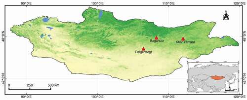
Figure 2. Satellite and on-site camera images of the ground sites: (a) Baganuur: BGN, (b) Delgertsogt: DGT, and (c) Khar yamaat: KYM. Satellite images were created from Sentinel-2A true colour images with the red squares representing the 500 m × 500 m areas covering the sites.

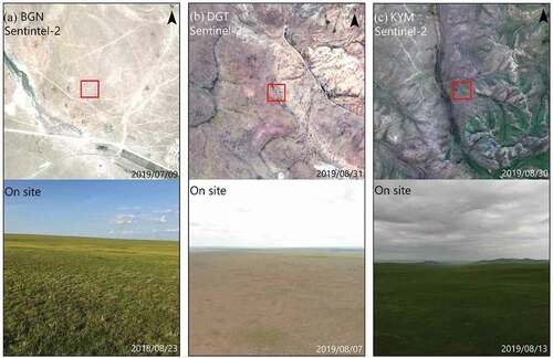
Table 1. Descriptions of the ground sites and the dates of in-situ and satellite observations.

Site ID	Site name	Latitude^1, longitude^1, altitude	Dominant vegetation species	Observation date^2 and local time
				in-situ	Satellite (SGLI)	Satellite (MODIS)
BGN	Baganuur	47°47‘53.3’’ N, 108°19‘51.5’’ E, 1396 m	Agropyron cristatum, Artemisia spp., Chenopodium spp., Cleistogenes squarrosa, Stipa krylovii	2018-08-22,　16:37–16:38 2018-08-23,　08:37–18:03 2018-08-24,　07:35–12:33	2018-08-24, 11:39	2018-08-24, 13:39
DGT	Delgertsogt	46°14‘56.0’’ N, 106°29‘42.9’’ E, 1380 m	Allium spp., Artemisia spp., Carex spp., Chenopodium spp., Salsora spp., Stipa krylovii	2019-08-08,　13:20–14:46 2019-08-09,　10:44–12:16	2019-08-09, 11:54 2019-08-10, 11:27	2019-08-09, 12:04 2019-08-10, 11:44
KYM	Khar yamaat	47°40‘13.8’’ N, 112°4‘34.9’’ E, 1060 m	Allium spp., Artemisia spp., Chenopodium spp., Cleistogenes squarrosa, Elymus chinensis, Potentilla acaulis, Stipa spp.	2019-08-13,　07:15–09:24	2019-08-13, 11:47	2019-08-13, 12:03

^aLatitude and longitude depict the location of the centres of the sites, described in WGS84.

^bDate is written according to ISO 8601.

For the national-scale study, the target area covers the entire Mongolia (approximately 1.565 × 10⁶ km², Figure 1). The climate is characterized by short, dry summers and long, cold winters. The ranges of the mean air temperatures across the northern to southern areas are 15°C to 25°C in summer and –15°C to –35°C in winter. The mean annual precipitation is 300–400 mm in the mountainous area, 150–250 mm in the Steppe, 100–150 mm in the mixed area of the Steppe and desert, and 50–100 mm in the desert (Gobi Desert) (Suttie 2005; Klinge et al. 2018).

2.2. Data

In the forthcoming sections, we will use a lot of types of VI and band reflectance derived from different sources. To avoid confusion, we define a rule to describe them in style as $V{I}_{sensor}^{origin}$ or $\mathrm{B}\mathrm{R}{n}_{sensor}^{origin}$, where VI is a vegetation index (either PRI or NDVI), the suffix ‘sensor’ is a satellite sensor (either SGLI or MODIS), the superfix ‘origin’ is the data origin (either ‘sat’ or ‘insitu’, meaning the data from a real satellite sensor or a simulation from in-situ data, respectively), BR means ‘band reflectance’, and n is the band identification number. For example, ‘${\mathrm{N}\mathrm{D}\mathrm{V}\mathrm{I}}_{\mathrm{M}\mathrm{O}\mathrm{D}\mathrm{I}\mathrm{S}}^{\mathrm{s}\mathrm{a}\mathrm{t}}$’ means the NDVI derived from the data taken by MODIS on the real Terra satellite, and ‘$\mathrm{B}\mathrm{R}{6}_{\mathrm{S}\mathrm{G}\mathrm{L}\mathrm{I}}^{\mathrm{i}\mathrm{n}\mathrm{s}\mathrm{i}\mathrm{t}\mathrm{u}}$’ means the simulated value of the band reflectance of SGLI band 6 (VN6) using in-situ spectral data. We sometimes omit ‘origin’ when the origin is obvious in the topic.

2.2.1. In-Situ data

(a) Spectral reflectance and band reflectance (BR):

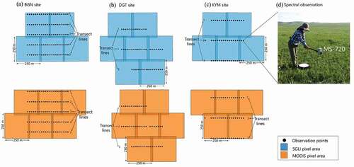
We observed the spectral reflectance and BR at three ground sites. We used a handheld spectroradiometer (MS-720, EKO Inc.) attached with a 45° collimation tube for the in-situ spectral reflectance observation. The specifications of the MS-720 were as follows: the spectral range of 350–1050 nm, the spectral interval of 3.3 nm, and the full width at half maximum of 10 nm. Spectral data at 3.3-nm intervals were converted to 1-nm intervals using the software accompanied with MS-720. The observations were conducted at 1-m above the ground at the points placed every 20 m along a transect line whose length was 400 m (Figure 3).

Figure 3. Transect lines and satellite pixels (Table 4) corresponding to the in-situ spectral observation points at the (a) BGN, (b) DGT, and (c) KYM sites. Black dots denote the spectral observation points. Black lines denote the transect lines. Blue and orange squares denote the 250 m × 250 m area around the pixel centres of the SGLI and MODIS images, respectively. (d) a picture of an in-situ spectral observation.

At each observation point, the spectral observation was conducted with the following sequence (let λ be wavelength): specifically, the spectral irradiance of sky-light L_sky1(λ), reflected light from the ground L_gr(λ), and again sky-light L_sky2(λ). The sky-light was observed as the reflected light from a calibrated white reference panel under a clear sky at the BGN site. At the DGT and KYM sites, the sky-light was observed directly by pointing the sensor upward under an overcast sky (assuming the homogeneous light intensity distribution in all the sky). The incoming sky-light L_sky(λ) was calculated as the mean of L_sky1(λ) and L_sky2(λ). The spectral reflectance R(λ) was calculated as R(λ)=L_gr(λ)/L_sky(λ). The $\mathrm{B}\mathrm{R}{n}_{sensor}^{\mathrm{i}\mathrm{n}\mathrm{s}\mathrm{i}\mathrm{t}\mathrm{u}}$, which is the band reflectance of the band n of a sensor (either SGLI or MODIS), was simulated using the in-situ spectral irradiance data as

(2) $\mathrm{B}\mathrm{R}{n}_{sensor}^{\mathrm{i}\mathrm{n}\mathrm{s}\mathrm{i}\mathrm{t}\mathrm{u}}=\frac{{\int }_{\lambda }{L}_{\mathrm{g}\mathrm{r}}\left(\lambda \right)\times \mathrm{R}\mathrm{S}\mathrm{R}{n}_{sensor}\left(\lambda \right)d\lambda }{{\int }_{\lambda }{L}_{\mathrm{s}\mathrm{k}\mathrm{y}}\left(\lambda \right)\times \mathrm{R}\mathrm{S}\mathrm{R}{n}_{sensor}\left(\lambda \right)d\lambda },$(2)

where RSRn_sensor(λ) is the relative spectral response of the band n of the sensor. The RSR of SGLI and MODIS was obtained from https://suzaku.eorc.jaxa.jp and https://oceancolor.gsfc.nasa.gov, respectively.

(b) Phenology data:

A time-lapse camera (Garden Watch Cam, Brinno Inc.) was installed at the BGN site to detect the dates of phenology events (DPE) (Nakano et al. 2020). The images were taken at 10-minute intervals in 2018.

(c) Meteorological data:

The air temperature and precipitation data were obtained from three Mongolian meteorological stations: Baganuur, Mandalgovi, and Bayan-Ovoo, close to the BGN, DGT, and KYM sites, respectively. The data are publicly available from the Information and Research Institute of Meteorology, Hydrology, and Environment.

2.2.2. Satellite data

In December 2018, JAXA released GCOM-C/SGLI standard products, such as the band reflectance and NDVI, on the Globe Portal System (G-Portal: https://gportal.jaxa.jp/). We used the products of SGLI and MODIS in 2018 and 2019 (Table 2). Before use, we shifted the SGLI image westward by a half-pixel. It was because JAXA announced a registration error occurred in the SGLI Level-2 products in version 1 (1001) and version 2 (2000), in which each pixel had been shifted a half-pixel eastward from the optimal position (Murakami 2021).

Table 2. Satellite data used in this study.

Satellite/sensor	Products	Spatial resolution	Version and period
GCOM-C/SGLI	GC1SG1 product Level 2 − Daily: NDVI; band reflectance of VN05^1, VN06, VN08, VN11, − 8-day statistics: NDVI (max); VN08 (max); VN11 (max)	250 m	Version 1 (1001): Jan. 2018–June 2019, Version 2 (2000): July 2019–Dec. 2019
Terra/MODIS	MOD09GQ − Daily: sur_refl_b01; sur_refl_b02,	250 m	Collection 6: 2018 and 2019
	MOD09Q 1− 8-day composite: sur_refl_b01; sur_refl_b02,
	MOD13Q1 − 16-day composite: NDVI
	MODOCGA − Daily: sur_refl_b11; sur_refl_b12	1000 m	Version 6: 2018 and 2019

^a‘VN’ is a prefix for GCOM-C SGLI band name, meaning ‘visible and near infrared’.

2.3. Definition of sensor-specific vegetation indices (VI)

The band reflectance depends on the RSR of each band of each sensor (Figure 4). Thus, each VI is specific to the sensor. Namely, even if a VI with the same name and concept is used, its characteristics are different among the sensors. In this study, we used PRI derived from SGLI (PRI_SGLI), PRI derived from MODIS (PRI_MODIS), NDVI derived from SGLI (NDVI_SGLI), and NDVI derived from MODIS (NDVI_MODIS).

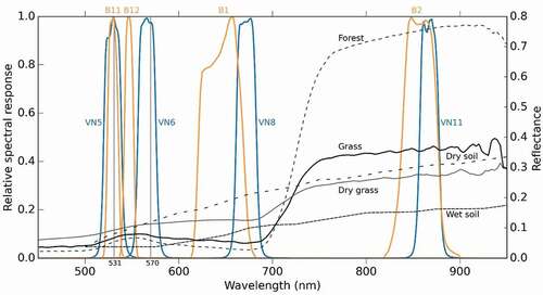
Figure 4. Relative spectral response (RSR) of SGLI (blue) and MODIS (yellow) in the wavelength between 500 nm 900 nm, along with typical examples of spectral reflectance of ground covers: grass canopy, dry grass canopy, dry soil, and wet soil. The reflectances of grass (LAI = 1.05) and dry grass (LAI = 0.18) canopies were measured at the Khar yamaat and Baganuur sites, respectively (in this study). The “dry grass canopy” means that the ground was covered with dry soil and sparse grass. The reflectance of the forest canopy was measured at a deciduous broad-leaved forest in Takayama, Japan (obtained from the Phenological Eyes Network, Nasahara and Nagai, 2015). The reflectance data from dry soil and wet soil was obtained from the literature (Baumgardner et al., 1986).

PRI_SGLI is defined by replacing R₅₃₁ with BR5_SGLI and R₅₇₀ with BR6_SGLI in Eq. (1). For PRI_MODIS, BR11_MODIS and BR12_MODIS are used, respectively. On the other hand, NDVI_SGLI and NDVI_MODIS are defined based on the definition of NDVI:

(3) $\mathrm{N}\mathrm{D}\mathrm{V}\mathrm{I}=\frac{\mathrm{B}\mathrm{R}\left(\mathrm{N}\mathrm{I}\mathrm{R}\right)-\mathrm{B}\mathrm{R}\left(\mathrm{r}\mathrm{e}\mathrm{d}\right)}{\mathrm{B}\mathrm{R}\left(\mathrm{N}\mathrm{I}\mathrm{R}\right)+\mathrm{B}\mathrm{R}\left(\mathrm{r}\mathrm{e}\mathrm{d}\right)},$(3)

where BR(red) and BR(NIR) are the band reflectance of red light and near-infrared light, respectively. For NDVI_SGLI, BR8_SGLI and BR11_SGLI are used for BR(red) and BR(NIR), respectively. For NDVI_MODIS, BR1_MODIS and BR2_MODIS are used, respectively.

We acquired the values of VIs (PRI_SGLI, NDVI_SGLI, and NDVI_MODIS) in two different independent approaches: in-situ observation and satellite observation. In the in-situ approach, we calculated (simulated) the VI values [using Equation (1)(1) $\mathrm{P}\mathrm{R}\mathrm{I}=\frac{{\mathrm{R}}_{531}-{\mathrm{R}}_{570}}{{\mathrm{R}}_{531}+{\mathrm{R}}_{570}},$(1) or Equation (3)(3) $\mathrm{N}\mathrm{D}\mathrm{V}\mathrm{I}=\frac{\mathrm{B}\mathrm{R}\left(\mathrm{N}\mathrm{I}\mathrm{R}\right)-\mathrm{B}\mathrm{R}\left(\mathrm{r}\mathrm{e}\mathrm{d}\right)}{\mathrm{B}\mathrm{R}\left(\mathrm{N}\mathrm{I}\mathrm{R}\right)+\mathrm{B}\mathrm{R}\left(\mathrm{r}\mathrm{e}\mathrm{d}\right)},$(3) ] from the in-situ band reflectance specific to each satellite sensor [calculated by Equation (2)(2) $\mathrm{B}\mathrm{R}{n}_{sensor}^{\mathrm{i}\mathrm{n}\mathrm{s}\mathrm{i}\mathrm{t}\mathrm{u}}=\frac{{\int }_{\lambda }{L}_{\mathrm{g}\mathrm{r}}\left(\lambda \right)\times \mathrm{R}\mathrm{S}\mathrm{R}{n}_{sensor}\left(\lambda \right)d\lambda }{{\int }_{\lambda }{L}_{\mathrm{s}\mathrm{k}\mathrm{y}}\left(\lambda \right)\times \mathrm{R}\mathrm{S}\mathrm{R}{n}_{sensor}\left(\lambda \right)d\lambda },$(2) ]. We call them ‘in-situ VI’. On the other hand, in the satellite approach, we either calculated the VI values [using Equation (1)(1) $\mathrm{P}\mathrm{R}\mathrm{I}=\frac{{\mathrm{R}}_{531}-{\mathrm{R}}_{570}}{{\mathrm{R}}_{531}+{\mathrm{R}}_{570}},$(1) or Equation (3)(3) $\mathrm{N}\mathrm{D}\mathrm{V}\mathrm{I}=\frac{\mathrm{B}\mathrm{R}\left(\mathrm{N}\mathrm{I}\mathrm{R}\right)-\mathrm{B}\mathrm{R}\left(\mathrm{r}\mathrm{e}\mathrm{d}\right)}{\mathrm{B}\mathrm{R}\left(\mathrm{N}\mathrm{I}\mathrm{R}\right)+\mathrm{B}\mathrm{R}\left(\mathrm{r}\mathrm{e}\mathrm{d}\right)},$(3) ] from the band reflectance products or just used NDVI products provided by the space agencies (Table 2). We call them ‘satellite VI’. The in-situ VIs was used as the reference data (validation data) for the satellite VIs.

2.4. Acquisition of the satellite VI

Using SGLI data and MODIS data, we acquired the values of satellite VI at each pixel covering each site (Figure 3). We acquired the satellite VI in three different time scales (daily, 8-day, and annual) for different purposes in different ways: (1) The daily VI data, calculated from the daily band reflectance data, were used for direct comparison with the in-situ VI data (the calculation was shown later). (2) The 8-day maximum NDVI data, derived from the daily NDVI data, were used for the time-series analysis. (3) The annual NDVI data, derived from the 8-day or 16-day time-series NDVI products, were used to compare SGLI and MODIS on the national scale. Table 3 explains all the cases.

Table 3. The satellite products used for deriving the satellite vegetation index (VI) and band reflectance (BR).

VI and BR	Sensor	Temporal resolution	Methods to obtain the VI and BR	Corresponding figures
PRI	SGLI	daily	calculated from band reflectance (VN5; VN6)	Figs. 7, 9, 11, 12
	MODIS	daily	calculated from band reflectance (band 11 and 12 of MODOCGA)	Figs. 7, 11
NDVI	SGLI	daily	calculated from band reflectance (VN8; VN11)	Figs. 6, 12
		8-day	8-day maximum of daily NDVI (mentioned above)	Figs. 7, 13
		annual	annual maximum of JAXA 8-day NDVI product	Figs. 14, 15
	MODIS	daily	calculated from band reflectance (band 1 and band 2 of MOD09GQ)	Fig. 6
		8-day	8-day maximum of daily NDVI (mentioned above)	Figs. 7, 13
		annual	annual maximum of NASA 16-day NDVI product (MOD13Q1)	Figs. 14, 15
BR	SGLI	daily	JAXA daily product (VN5; VN6; VN8; VN11)	Fig. 12
		8-day	JAXA 8-day product (max VN8; max VN11)	Fig. 7
	MODIS	daily	MODOCGA (band 11; band 12)	Fig. 7
		8-day	MOD09Q1 (band 1; band 2)	Fig. 7

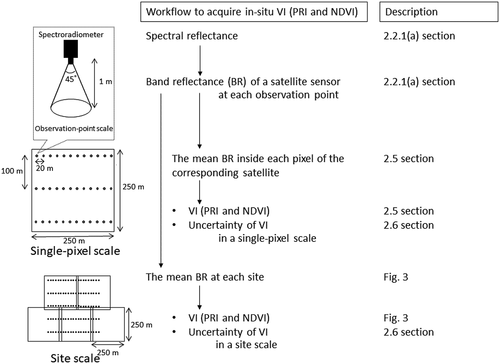
2.5. Acquisition of the in-situ VI in a single-pixel scale corresponding to a satellite

Each site was covered with multiple pixels of a satellite sensor (such as five SGLI pixels covering the BGN site, Figure 3 and Table 4). Therefore, we calculated each in-situ VI for each pixel of the corresponding satellite (such as five PRI_SGLI values at the BGN site).

Table 4. Coordinate of the pixels within the satellite product tile (04, 25) (vertical tile number, horizontal tile number) used in this study.

Site	Sensor	Sample size	Row and column within the 0425 tile
BGN	SGLI	5	(1056, 1329), (1056, 1330), (1057, 1330), (1057, 1331), (1057, 1332)
	MODIS	6	(1056, 1328), (1056, 1329), (1056, 1330), (1057, 1329), (1057, 1330), (1057, 1331)
DGT	SGLI	7	(1799, 1747), (1799, 1748), (1800, 1748), (1800, 1749), (1800, 1750), (1801, 1751), (1801, 1750)
	MODIS	7	(1799, 1747), (1799, 1748), (1800, 1748), (1800, 1749), (1800, 1750), (1801, 1750), (1801, 1751)
KYM	SGLI	5	(1117, 2624), (1117, 2625), (1118, 2625), (1118, 2626), (1118, 2627)
	MODIS	5	(1117, 2624), (1117, 2625), (1117, 2626), (1118, 2626), (1118, 2627)

The procedure to acquire the in-situ VI is as follows, also shown in Figure 5: First, we calculated the band reflectance, specific to each satellite sensor, at each observation point using the in-situ data and Equation (2)(2) $\mathrm{B}\mathrm{R}{n}_{sensor}^{\mathrm{i}\mathrm{n}\mathrm{s}\mathrm{i}\mathrm{t}\mathrm{u}}=\frac{{\int }_{\lambda }{L}_{\mathrm{g}\mathrm{r}}\left(\lambda \right)\times \mathrm{R}\mathrm{S}\mathrm{R}{n}_{sensor}\left(\lambda \right)d\lambda }{{\int }_{\lambda }{L}_{\mathrm{s}\mathrm{k}\mathrm{y}}\left(\lambda \right)\times \mathrm{R}\mathrm{S}\mathrm{R}{n}_{sensor}\left(\lambda \right)d\lambda },$(2) . Then, we took their mean of the band reflectance at all points inside each pixel of the corresponding satellite (Figure 3). Considering the non-linearity of the relationship between fractional ground cover and VI (e.g. Jones and Vaughan 2010), we acquired the in-situ VI in the single-pixel scale by putting the inside-pixel mean values of the band reflectance into the definition of the VIs. As a result, we obtained a pair of satellite VI and in-situ VI for each pixel in each site. The pairs allowed us to compare the satellite VI and the in-situ VI at the single-pixel level.

Figure 5. Workflow to acquire the in-situ vegetation index (VI, PRI, and NDVI).

2.6. Calculation of the uncertainty of VI

The uncertainty of the in-situ VI (for a single-pixel scale and a site scale) and the satellite VI (for a site scale) was estimated by the uncertainty propagation theory as follows: Let u(x, y) be the function, which defines a VI as follows:

(4) $u\left(x,y\right)=\left(x-y\right)/\left(x+y\right),$(4)

where x and y are the mean band reflectance. The VI’s uncertainty (σ) can be calculated from the band reflectance’s uncertainty, which is expressed by the standard error of x and y (denoted by σ_x and σ_y, respectively):

(5) ${\sigma }^2={\left(\frac{\mathrm{\partial }u}{\mathrm{\partial }x}{\sigma }_x\right)}^2+{\left(\frac{\mathrm{\partial }u}{\mathrm{\partial }y}{\sigma }_y\right)}^2(Formulaofuncertaintypropagation)=\frac{4y^2}{{\left(x+y\right)}^4}\left({{\sigma }_x}^2+{{\sigma }_y}^2\right),$(5)

(6) $\sigma =\frac{2y}{{\left(x+y\right)}^2}\sqrt{{{\sigma }_x}^2+{{\sigma }_y}^2.}$(6)

Each of σ_x and σ_y was calculated as

(7) ${\sigma }_b=\frac{std}{\sqrt{n}},$(7)

where b is either x or y, std is a standard deviation of b, and n is the number of observation points inside a pixel.

2.7. Detection of dates of phenological events (DPE)

2.7.1. DPE detection from in-situ data

We empirically detected five types of DPE for the target year using a time-lapse camera: the starting and ending dates of the growing season (GS_s and GS_e, respectively), the peak date of the growing season (GS_p), and the starting and ending dates of the snowmelt (SM_s and SM_e, respectively). This method has been applied to detect the ground truth DPE (Xie, Civco, and Silander 2018; Ide and Oguma 2010; Lim et al. 2018; Yan et al. 2019). The length of the growing season (LGS; unit: days) was equated to the number of days between the GS_e and GS_s as follows:

(8) $\mathrm{L}\mathrm{G}\mathrm{S}=\mathrm{G}{\mathrm{S}}_{\mathrm{e}}-\mathrm{G}{\mathrm{S}}_{\mathrm{s}}+1.$(8)

2.7.2. DPE detection from satellites

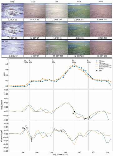
We also detected the DPE of the growing season (GS_s, GS_e, and GS_p) from the time series of NDVI, which was temporally smoothed by a Savitzky-Golay filter (Chen et al. 2004) with the window length of 5, at the BGN site in 2018 as follows: (i) The inflection point (the maxima of the second derivative) during the spring (from May to July) was identified as the GS_s (Gong et al. 2015); (ii) The other inflection point (the minimum of the first derivative) during the autumn (from August to October) was identified as the GS_e; (iii) The GS_p was defined as the date of the maximum NDVI (the zero point of the first derivative) during the growing season (Gong et al. 2015). In addition, we detected the DPE of the snowmelt (SM_s, and SM_e) from the NDVI time series as follows: (iv) The inflection point (the maxima of the second derivative) during the end of the winter (from February to March was identified as the SM_s, while another inflection point (the minimum of the second derivative) during the end of the winter (from February to March) was identified as the SM_e (e.g. Zhang et al. 2003).

2.8. Comparison of NDVI of SGLI and MODIS on the national scale

For the long-term analysis of NDVI time series, the combination uses of NDVI derived from multiple sensors is useful. However, the characteristics of NDVI are different among the sensors. To identify the difference of NDVI between SGLI and MODIS, we compared NDVI_SGLI and NDVI_MODIS. The comparison was conducted for the annual maxima of NDVI_SGLI and NDVI_MODIS in 2019 throughout Mongolia and for each Mongolian natural zone: (a) forest-steppe and mountain-taiga, (b) steppe, (c) semi-desert steppe, and (d) desert. Although NDVI_SGLI and NDVI_MODIS have the same spatial resolution, the locations of the grids of the pixels are slightly different from each other. Therefore, we resampled both NDVI_SGLI and NDVI_MODIS images onto the same grids by the ‘average resampling’ method, which computes the weighted average of all contributing pixels, using the ‘gdalwarp’ command in the Geospatial Data Abstraction Library before the comparison.

3. Results

3.1. Comparison of the satellite NDVI and the in-situ NDVI

The correlation between the satellite NDVI and in-situ NDVI was high throughout all sites: The correlation coefficient (R) was 0.988 and 0.994 for SGLI and MODIS, respectively, when the satellite NDVI was taken on the closest sunny day to the day of the in-situ observation (Figure 6). As for the DGT site, the closest sunny day was different from SGLI and MODIS. SGLI data had cloud flags on the same day as the in-situ observation (August 09, 2019), although the MODIS had no cloud flags (August 09, 2019). Therefore, for reference, we also calculated the R using SGLI data despite having cloud flags on August 09, 2019. The accuracy of ${\mathrm{N}\mathrm{D}\mathrm{V}\mathrm{I}}_{\mathrm{S}\mathrm{G}\mathrm{L}\mathrm{I}}^{\mathrm{s}\mathrm{a}\mathrm{t}}$ may be acceptable even in a case having cloud flags. Although the accuracy of the data with cloud flags (August 09, 2019) was worse than the data with no cloud flags (August 10, 2019), the root-mean-square error (RMSE) was better than MODIS with no cloud flags (August 09, 2019): The RMSE was 0.090 for SGLI and 0.163 for MODIS (Figure 6a,b).

Figure 6. Comparison of the in-situ NDVI and the satellite NDVI: (a) GCOM-C/SGLI and (b) Terra/MODIS. The satellite NDVI was taken on the closest sunny day to the day of the in-situ observation. The RMSE for all data was calculated using 1) BGN, DGT (satellite data on 2019-08-09), and KYM data and 2) BGN, DGT (satellite data on 2019-08-10), and KYM data. For the DGT site, the satellite NDVI of two days (the closest sunny day for both SGLI and MODIS: 2019-08-10 and the same day with the in-situ observation: 2019-08-09, cloudy for SGLI and sunny for MODIS) was demonstrated. The bar denotes the uncertainty of the in-situ mean PRI calculated by Eq. 6(6) $\sigma =\frac{2y}{{\left(x+y\right)}^2}\sqrt{{{\sigma }_x}^2+{{\sigma }_y}^2.}$(6) .

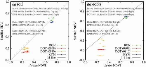
On a closer look at the data on each site, in the case of SGLI, the satellite NDVI was nearly on the 1:1 line at the BGN site, where the sky-light was observed using the calibrated white reference panel (RMSE = 0.033, Table 5). In contrast, it tended to be slightly lower than the in-situ NDVI at the DGT and KYM sites, where the sky-light was observed without using the white reference panel (Table 6). In the case of MODIS, no such pattern did not appear at the KYM data. It might matter little whether using the white reference panel or not. In a semi-desert Steppe site (DGT), covered with sparse vegetation, SGLI was better in both R and RMSE than MODIS (Table 5). In contrast, in a higher vegetation-covered area (KYM), SGLI was slightly worse in RMSE but better in R than MODIS (Table 5).

Table 5. The correlation coefficient and the root-mean-square error between the in-situ vegetation index (VI) and satellite VI at each observation site.

Site	In-situ observation	Satellite		NDVI		PRI
	Date, condition	Sensor	Date, condition	RMSE	R	RMSE	R
BGN	2018-08-22/24, sunny	SGLI	2018-08-24, no cloud	0.033	0.048	0.052	−0.76
		MODIS	2018-08-24, no cloud	0.027	0.53	NA	NA
DGT	2019-08-08/09, cloudy, drizzly	SGLI	2019-08-09, cloud	0.128	0.66	0.021	−0.48
			2019-08-10, no cloud	0.078	−0.017	0.047	0.42
		MODIS	2019-08-09, no cloud	0.259	−0.20	NA	NA
			2019-08-10, no cloud	0.231	−0.21	NA	NA
KYM	2019-08-13, sunny	SGLI	2019-08-13, no cloud	0.062	0.96	0.069	0.52
		MODIS	2019-08-13, no cloud	0.016	−0.89	NA	NA

Table 6. Comparison of NDVI_SGLI and NDVI_MODIS simulated using the spectral reflectance of a forest canopy, grass, dry grass, wet soil, and dry soil, which is described in Fig. 4.

Type of ground cover	NDVISGLI	NDVIMODIS
Forest canopy	0.93	0.91
Grass canopy	0.74	0.71
Dry soil and dry grass	0.35	0.33
Wet soil	0.22	0.31
Dry soil	0.16	0.21

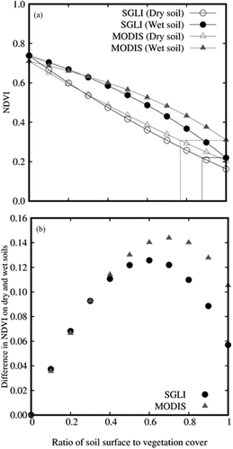
The time series of the satellite NDVI (Figure 7) showed a general seasonal pattern, which is small in winter and large in summer. In more detail, the increase of NDVI followed the increase of precipitation rather than the increase of air temperature, implying a stronger control by water than temperature. Although such patterns were common in NDVI_SGLI and NDVI_MODIS, NDVI_SGLI tended to be slightly lower than NDVI_MODIS in the early growing season and higher in the late growing season (Figure 7). This tendency depends on the wavelength range of the red band and that of the NIR band (Figure 4). For instance, NDVI_SGLI is slightly lower than NDVI_MODIS on the soil surface (Table 6). Such a relationship continues until the vegetation-cover fraction reaches 0.7 ( = 0.3 of soil fraction) (e.g. see the relationship between solid triangles and solid circles in Figure 8a). This case can apply to the early growing season in Mongolian grassland. The late growing season is another case. When the vegetation-cover fraction at the peak, NDVI_SGLI is slightly higher than NDVI_MODIS until the fraction reaches 0.7 (Figure 8).

Figure 7. Time-Series of temperature, precipitation, NDVI, and PRI (a) at the BGN site in 2018, (b) at the DGT site in 2019, and (c) at the KYM site in 2019. The in-situ data (shown by the large circles and the large triangles) are the mean of NDVI or PRI within a target area (shown in Fig. 3) at each study site. The bars of the vegetation index and band reflectance denote the uncertainty of the mean (calculated by Eq. 6(6) $\sigma =\frac{2y}{{\left(x+y\right)}^2}\sqrt{{{\sigma }_x}^2+{{\sigma }_y}^2.}$(6) ) and the standard error, respectively.

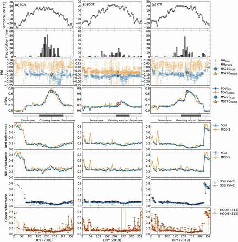
Figure 8. Comparison of NDVI_SGLI with NDVI_MODIS on (a) the relationship between NDVI and the ratio of the soil surface to vegetation cover in wet and dry soils (b) the difference in NDVI on dry and wet soils. The simulation was conducted using the spectral reflectance of grass, wet soil, and dry soil, which are described in Fig. 4.

3.2. Comparison of satellite PRI with in-situ PRI

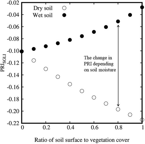
The comparison of ${\mathrm{P}\mathrm{R}\mathrm{I}}_{\mathrm{S}\mathrm{G}\mathrm{L}\mathrm{I}}^{\mathrm{s}\mathrm{a}\mathrm{t}}$ and ${\mathrm{P}\mathrm{R}\mathrm{I}}_{\mathrm{S}\mathrm{G}\mathrm{L}\mathrm{I}}^{\mathrm{i}\mathrm{n}\mathrm{s}\mathrm{i}\mathrm{t}\mathrm{u}}$ at all three sites yielded a low correlation: Although the RMSE was small at all three sites, the R was negative (Table 5, Figure 9). The negative correlation might be attributed to the moisture change in the soil uncovered by sparse and patchy vegetation. The simulation demonstrated that $\mathrm{P}\mathrm{R}{\mathrm{I}}_{\mathrm{S}\mathrm{G}\mathrm{L}\mathrm{I}}$ was larger on the wet soil and smaller on the dry soil (Figure 10), indicating that the moisture change in the soil has a larger influence on $\mathrm{P}\mathrm{R}{\mathrm{I}}_{\mathrm{S}\mathrm{G}\mathrm{L}\mathrm{I}}$ in a smaller vegetation-cover fraction. The increase of RMSE on a sunny day but one day after the in-situ observation might be attributable to the rapid change of soil moisture after drizzle at the semi-desert steppe site (DGT) (Figure 9, Table 5). Even when successfully comparing ${\mathrm{P}\mathrm{R}\mathrm{I}}_{\mathrm{S}\mathrm{G}\mathrm{L}\mathrm{I}}^{\mathrm{i}\mathrm{n}\mathrm{s}\mathrm{i}\mathrm{t}\mathrm{u}}$ with ${\mathrm{P}\mathrm{R}\mathrm{I}}_{\mathrm{S}\mathrm{G}\mathrm{L}\mathrm{I}}^{\mathrm{s}\mathrm{a}\mathrm{t}}$ on the same day, the R was small (0.34). It implies that the gap in the timing of observation between the satellite and the ground (in-situ) also prevents the success of the accuracy assessment (see Table 1) because PRI can change rapidly even within a day in response to the physiological dynamics of plants (Wong and Gamon 2015; Gitelson, Gamon, and Solovchenko 2017) and the moisture change in the soil (this study). Because of the rapid change of PRI, the direct comparison of ${\mathrm{P}\mathrm{R}\mathrm{I}}_{\mathrm{S}\mathrm{G}\mathrm{L}\mathrm{I}}^{\mathrm{s}\mathrm{a}\mathrm{t}}$ and ${\mathrm{P}\mathrm{R}\mathrm{I}}_{\mathrm{S}\mathrm{G}\mathrm{L}\mathrm{I}}^{\mathrm{i}\mathrm{n}\mathrm{s}\mathrm{i}\mathrm{t}\mathrm{u}}$ has difficulty in terms of synchroneity.

Figure 9. Comparison of the in-situ PRI_SGLI and the satellite PRI_SGLI at all sites. The satellite PRI was taken on the closest sunny day to the day of the in-situ observation. For the DGT site, the satellite PRI of two days (the closest sunny day: 2019-08-10 and the same day with the in-situ observation but cloudy: 2019-08-09) was demonstrated. The RMSE for all data was calculated using 1) BGN, DGT (satellite data on 2019-08-09), and KYM data and 2) BGN, DGT (satellite data on 2019-08-10), and KYM data.

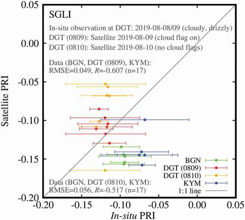
Figure 10. Relationship between PRI_SGLI and the ratio of the soil surface to vegetation cover on dry and wet soils. The simulation was conducted using the spectral reflectance of grass, wet soil, and dry soil, which are described in Fig. 4.

Instead of the direct comparison, we checked how the time series of the satellite PRI of SGLI (${\mathrm{P}\mathrm{R}\mathrm{I}}_{\mathrm{S}\mathrm{G}\mathrm{L}\mathrm{I}}^{\mathrm{s}\mathrm{a}\mathrm{t}}$) changes depending on the precipitation and air temperature. As a result, although ${\mathrm{P}\mathrm{R}\mathrm{I}}_{\mathrm{S}\mathrm{G}\mathrm{L}\mathrm{I}}^{\mathrm{s}\mathrm{a}\mathrm{t}}$ showed different seasonality between the study sites, it showed a common feature in which it decreased after the peak of the precipitation season (Figure 7). In fact, ${\mathrm{P}\mathrm{R}\mathrm{I}}_{\mathrm{S}\mathrm{G}\mathrm{L}\mathrm{I}}^{\mathrm{s}\mathrm{a}\mathrm{t}}$ at the BGN site was stable until DOY 220 (Figure 7), but after the precipitation peak (DOY 225), it started decreasing. Concurrently with the end of precipitation (DOY 280), it reached a minimum, and then it started increasing. After the start of the snow season, it stopped increasing. At the DGT site, although ${\mathrm{P}\mathrm{R}\mathrm{I}}_{\mathrm{S}\mathrm{G}\mathrm{L}\mathrm{I}}^{\mathrm{s}\mathrm{a}\mathrm{t}}$ exhibited relatively less volatility in the seasonality than the BGN sites, its peak appeared concurrently with the peak of precipitation (DOY 225), and then it started decreasing. At the KYM site, PRI_SGLI showed little seasonality until the end of the precipitation season (DOY 250), when it started decreasing. During the snow season, PRI_SGLI was unstable, showing big fluctuations (Figure 7c).

For reference purposes, we demonstrated the time series of the satellite PRI of MODIS (${\mathrm{P}\mathrm{R}\mathrm{I}}_{\mathrm{M}\mathrm{O}\mathrm{D}\mathrm{I}\mathrm{S}}^{\mathrm{s}\mathrm{a}\mathrm{t}}$) using ocean bands 11 and 12 (Figure 7). Unlike ${\mathrm{P}\mathrm{R}\mathrm{I}}_{\mathrm{S}\mathrm{G}\mathrm{L}\mathrm{I}}^{\mathrm{s}\mathrm{a}\mathrm{t}}$, ${\mathrm{P}\mathrm{R}\mathrm{I}}_{\mathrm{M}\mathrm{O}\mathrm{D}\mathrm{I}\mathrm{S}}^{\mathrm{s}\mathrm{a}\mathrm{t}}$ did not show a seasonal pattern at any sites. Especially at the BGN and KYM sites, the fluctuations were too large to detect the seasonality.

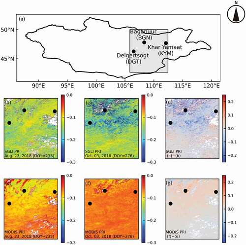
We created the spatial distribution maps of the satellite PRI of SGLI (${\mathrm{P}\mathrm{R}\mathrm{I}}_{\mathrm{S}\mathrm{G}\mathrm{L}\mathrm{I}}^{\mathrm{s}\mathrm{a}\mathrm{t}}$) in late August (the peak of greenness) and early October (the terminal of the precipitation season) in a rectangle area including the three study sites (Figure 11). Inside this area, in a steppe region extending from the centre to the east, PRI was high in late August (Figure 11b) and low in early October (Figure 11c). PRI in the northern region (the forests) also changed from high to low. In contrast, in the southern region (the desert), PRI showed little changes between the two seasons. For reference purposes, we also created the spatial distribution map of the satellite PRI of MODIS (${\mathrm{P}\mathrm{R}\mathrm{I}}_{\mathrm{M}\mathrm{O}\mathrm{D}\mathrm{I}\mathrm{S}}^{\mathrm{s}\mathrm{a}\mathrm{t}}$) (the lowest figures in Figure 11). The spatial distribution was different from ${\mathrm{P}\mathrm{R}\mathrm{I}}_{\mathrm{S}\mathrm{G}\mathrm{L}\mathrm{I}}^{\mathrm{s}\mathrm{a}\mathrm{t}}$ (Figure 11). The seasonal change of ${\mathrm{P}\mathrm{R}\mathrm{I}}_{\mathrm{M}\mathrm{O}\mathrm{D}\mathrm{I}\mathrm{S}}^{\mathrm{s}\mathrm{a}\mathrm{t}}$ seems almost opposite to ${\mathrm{P}\mathrm{R}\mathrm{I}}_{\mathrm{S}\mathrm{G}\mathrm{L}\mathrm{I}}^{\mathrm{s}\mathrm{a}\mathrm{t}}$: PRI was lower in late August (Figure 11e) and higher in early October (Figure 11F). However, since the fluctuation was too large in the time series (Figure 7), the seasonal change and the spatial distribution patterns might possess lower reliability.

Figure 11. Spatial distribution of PRI derived from SGLI in (a) the area including three study sites on (b) August 23, 2018 (the peak of greenness), and (c) October 03, 2018 (the end of the growing season). (d) Subtraction of (b) from (c).

3.3. Accuracy assessment of each band reflectance of SGLI

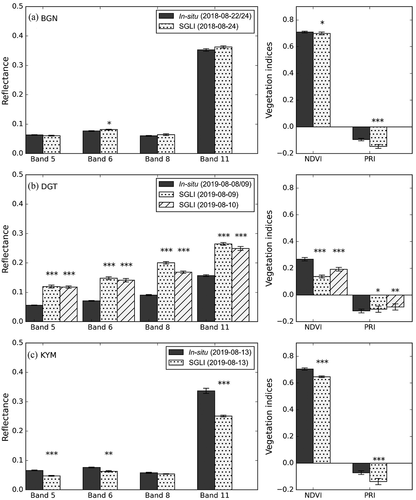
We compared each band reflectance derived from SGLI with in-situ data to seek the cause of the discrepancy in PRI and NDVI of SGLI. At the BGN site, all bands had no significant discrepancy in reflectance except a green band (Band 6, Figure 12a). In contrast, there was a discrepancy in all bands except the red band (Band 8) at the KYM site (Figure 12c). At the semi-desert steppe site (DGT), the discrepancy was the largest: All four bands had a significant discrepancy in reflectance (Figure 12b). It is attributable to the time gap between the in-situ observation (August 08–09, 2019 [drizzle]) and satellite observation (August 10, 2019 [no cloud flag]) at the DGT site (Table 1). That is, the soil surface condition changed from wet (at the in-situ observation) to dry (at the satellite observation). This result implies the soil surface condition largely affects the reflectance in the sparse vegetation.

Figure 12. Comparison of the band reflectance between the SGLI (satellite data) and the MS-720 spectroradiometer (in-situ data) at the (a) BGN, (b) DGT, and (c) KYM sites. The daily SGLI band reflectance data were taken on the closest sunny day to the day of the in-situ observation. For the DGT site, the SGLI data of two days (the closest sunny day: 2019-08-10 and the same day with the in-situ observation but cloudy: 2019-08-09) was demonstrated. The bars for the band reflectance and the VI denote the standard error of the mean and the uncertainty of the mean (calculated by Eq. 6(6) $\sigma =\frac{2y}{{\left(x+y\right)}^2}\sqrt{{{\sigma }_x}^2+{{\sigma }_y}^2.}$(6) ) within the target area at each observation site, respectively. The *, **, and *** indicate p-values less than 0.05, 0.01, and 0.001, respectively (Welch’s t-test).

3.4. Evaluation of DPE detected from SGLI

We compared the DPE (SGLI) with the reference DPE (time-lapse camera) (Figure 13). As a result, SGLI could accurately detect most of the DPE: the growing season GS_s (start), GS_p (peak), GS_e (end), and the snowmelt SM_s (start). The discrepancies were less than a few days. One exception was the end of the snowmelt (SM_e). It was detected slightly late (six days later). MODIS also accurately detected GS_p within a few days. However, the discrepancies were larger than SGLI DPE: For instance, as for MODIS DPE, GS_e was ten days earlier, and GS_s was 26 days later. As a result, the detection accuracy in SGLI DPE was as good or better compared to the detection in MODIS DPE.

Figure 13. Dates of phenological events (DPE) detected from the in-situ observation (time-lapse camera) and the satellite time-series NDVI at the BGN site in 2018. The time-lapse camera images, shown above the graphs, were taken on the DPE detected from three sources (camera, NDVI_SGLI, and NDVI_MODIS). The blue line denotes the NDVI_SGLI, and the orange line is the NDVI_MODIS.

3.5. Consistency of NDVI_SGLI and NDVI_MODIS on the national scale

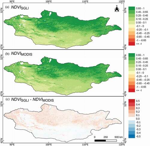
We evaluated the consistency of NDVI_SGLI with NDVI_MODIS using the annual maximum NDVI, relating to the maximum amount of vegetation. As a result, the consistency of NDVI_SGLI with NDVI_MODIS was high: Throughout Mongolia, the correlation was the highest (R² = 0.93, Figure 14b). It was also high in grassland (steppe and semi-desert steppe) (R² was more than 0.81, Figure 14d and 14e). In contrast, it was relatively low in the forest zones (mountain-taiga and forest-steppe) (R² was 0.75, Figure 14c).

Figure 14. Comparison of the annual maximum NDVI of SGLI and MODIS in 2019 in each natural zone [delineated in (a)] of Mongolia (Dash, 2005): (b) the entire of Mongolia, (c) mountain-taiga and forest-steppe, (f) steppe, (e) semi-desert, and (f) desert. The colour bar denotes the number of pixels. The dashed line in a scatter diagram is the 1:1 line. (g)–(j) Images of typical vegetation cover of each natural zones.

We found the differences of the annual maximum NDVI_SGLI from the NDVI_MODIS as follows: The annual maximum NDVI_SGLI was larger than the NDVI_MODIS in the area covered with vegetation (forests and steppes) (Figure 15). Particularly in forests, NDVI_SGLI was obviously large (Figure 14c and 15). The large differences mostly appeared in the western and northern areas in Mongolia, where high mountains (i.e. sparse vegetation) and taiga are distributed (Figure 15c).

Figure 15. Spatial distributions of the annual maxima of (a) NDVI_SGLI, (b) NDVI_MODIS, and (c) the difference in 2019.

To clarify the characteristics mentioned above, we compared the NDVI_SGLI and NDVI_MODIS simulated using the RSR and the spectral reflectance of the typical ground conditions shown in Figure 4. As a result (Table 6), when the ground was vegetated (i.e. ‘forest canopy’, ‘grass canopy’, and ‘dry soil and grass’ in Figure 4), NDVI_SGLI was higher than NDVI_MODIS. In contrast, when the ground was non-vegetated (i.e. ‘wet soil’ and ‘dry soil’ in Figure 4), NDVI_SGLI was lower than NDVI_MODIS. It means that NDVI_SGLI might be better to classify vegetated and non-vegetated ground than NDVI_MODIS. In fact, NDVI_SGLI is distinctively larger in the vegetated ground than the non-vegetated ground. In contrast, NDVI_MODIS is sometimes the approximately same between the vegetated ground and the non-vegetated ground (NDVI_MODIS ≈0.3 for both ‘dry soil and grass’ and ‘wet soil’ in Table 6). This fact may be due to the higher sensitivity of NDVI_MODIS to soil wetness: From dry soil to wet soil, NDVI_MODIS makes a bigger change than NDVI_SGLI at small vegetation coverages (Figure 8b). Accordingly, NDVI_MODIS requires more careful attention to soil wetness than NDVI_SGLI at small vegetation coverages: As for SGLI, NDVI on the wet soil is smaller than NDVI at 15% vegetation coverage on the dry soil (see a dashed line for SGLI in Figure 8a). As for MODIS, it is larger than NDVI even at 20% vegetation coverage on the dry soil (see a dashed line for MODIS in Figure 8a).

4. Discussion

PRI is an index to detect the xanthophyll cycle, which results in the release of excess light energy under strong light and water-stressed conditions (e.g. Demmig-Adams and Adams III 1992; Filella et al. 2004; Mänd et al. 2010). We also demonstrated that the time series of ${\mathrm{P}\mathrm{R}\mathrm{I}}_{\mathrm{S}\mathrm{G}\mathrm{L}\mathrm{I}}^{\mathrm{s}\mathrm{a}\mathrm{t}}$ had the potential to detect the water stress of vegetation (i.e. stress due to dryness) in this study. Because when warm air temperatures and relatively high NDVI are ongoing, ${\mathrm{P}\mathrm{R}\mathrm{I}}_{\mathrm{S}\mathrm{G}\mathrm{L}\mathrm{I}}^{\mathrm{s}\mathrm{a}\mathrm{t}}$ started decreasing after the end of the precipitation season at all study sites around DOY 225–250 (Figure 7). However, in this early validation study, we could not demonstrate the high accuracy of the satellite PRI_SGLI with the in-situ PRI_SGLI. In fact, the R between the satellite and in-situ PRI_SGLI was negative. The negative correlation might be caused by the rapid change of PRI and the time gap between the in-situ and satellite observations. Especially in Mongolian dry grassland, the moisture change in the soil surface uncovered by sparse and patchy vegetation affects PRI. In spite of poor correlation, on a site scale, the mean of the in-situ PRI_SGLI was within the range of seasonal variation of the satellite PRI_SGLI in each ground site (Figure 7). Besides, the negative correlation might be caused by the registration error that happened in the early SGLI products. Further study is expected for PRI validation in the future.

The readers may think PRI can be detected from MODIS’s two green ocean bands (11 and 12), although its spatial resolution (1 km) is coarser than SGLI’s (250 m). However, the PRI_MODIS (bands 11 and 12) was too noisy to detect the seasonal variation (Middleton et al. 2016, and this study) because of the noise in each band signal (Figure 7).

In this study, we also evaluated the accuracy of the satellite NDVI_SGLI using the in-situ NDVI_SGLI as a reference. The accuracy was high at all three ground sites (Figure 6a). However, a closer look revealed that the in-situ NDVI_SGLI was slightly higher than the satellite NDVI_SGLI at the two ground sites (DGT and KYM). The slightly high ${\mathrm{N}\mathrm{D}\mathrm{V}\mathrm{I}}_{\mathrm{S}\mathrm{G}\mathrm{L}\mathrm{I}}^{\mathrm{i}\mathrm{n}\mathrm{s}\mathrm{i}\mathrm{t}\mathrm{u}}$ was observed on the wet ground at the two sites. Since the ground was not entirely covered with vegetation (LAI is less than 1.0), the ground condition must influence NDVI in grassland (Miller 1977). In fact, NDVI on the wet ground was higher than NDVI on the dry ground (Table 6) because the reflectance of NIR increases with the soil moisture (Jones and Vaughan 2010).

On the other hand, the accuracy of the band reflectance showed the same tendency as the accuracy of NDVI_SGLI. That is the accuracy was the highest at the BGN site and relatively low at the other two sites (DGT and KYM). It might be attributable to the bad sky condition at the observation (a mist and a morning dew) and the wet soil condition at the two sites.

As for the consistency between the NDVI_SGLI and NDVI_MODIS, the annual maxima of the NDVI_SGLI and NDVI_MODIS were consistent with each other (Figure 14 and 15). However, the characteristics were slightly different. The comparative relation between NDVI_SGLI and NDVI_MODIS reversed depending on whether the ground was covered with vegetation or non-vegetation: The annual maxima NDVI_SGLI tended to be larger than the NDVI_MODIS in the vegetated ground and smaller in the non-vegetated ground (Figure 15c, Table 6). In the Mongolian desert, the ground was covered with dry soil and some patchy vegetation (see Figure 14j). Accordingly, the reverse relationship might lead to the relatively low correlation of NDVI in the desert (Figure 14F). Besides, the changing rate of NDVI in response to the soil moisture was different: NDVI_SGLI had a smaller response to the soil moisture than NDVI_MODIS (Figure 15). The smaller response might allow NDVI_SGLI to better classify vegetated and non-vegetated ground than NDVI_MODIS in sparse grassland. In contrast, since NDVI_MODIS was sometimes the same between the vegetated ground and the non-vegetated ground (see a dashed line for MODIS in Figure 8a), it is difficult to classify them using NDVI_MODIS in sparse vegetation.

Lastly, we checked the accuracy of the DPE detection from the time series of NDVI_SGLI. The DPE of the growing season (GS_s, GS_p, and GS_e) were accurately detected (Figure 13). Also, the DPE of snowmelt (SM_s and SM_e) detected from the time series of NDVI_SGLI can be acceptable. There were no large discrepancies between DPE detections from NDVI_SGLI and NDVI_MODIS, except for the detection of GS_s. NDVI_SGLI might be more sensitive to the increase of greenness in case of low vegetation coverage than NDVI_MODIS. The discrepancies are attributable to the difference in the wavelength range of the red band. In fact, the SGLI red band is narrower and closer to the red edge (680–750 nm) than MODIS red band (Figure 4). It might make the slightly different seasonal pattern of NDVI between SGLI and MODIS.

5. Conclusions

We presented the validation results of the PRI and NDVI derived from a new satellite GCOM-C in the initial stage. We validated the accuracy using in-situ data obtained by the field campaign at Mongolian grasslands. The followings are our findings:

• GCOM-C/SGLI provides corresponding spectral bands to derive PRI.

• PRI_SGLI showed clear seasonality depending on the water stress of vegetation: It was high in summer and decreased after the peak of the precipitation season. In contrast, PRI_MODIS (using ocean bands 11 and 12) did not show such seasonality.

• In the desert region, PRI_SGLI showed little changes between summer and autumn.

• In sparse vegetation, PRI_SGLI largely varied depending on the soil moisture. Accordingly, the correlation between in-situ and satellite PRI was negative because of the time lag in observation.

• GCOM-C/SGLI provided a reliable NDVI in Mongolian grasslands.

• NDVI_SGLI could detect the phenology as competent as NDVI_MODIS.

• NDVI_SGLI has enough similarities with NDVI_MODIS in terms of accuracy, spatial resolution, and frequency. Thus, it can play a role as the successor to NDVI_MODIS in global plant study.

• The dependency of NDVI_SGLI on the soil moisture was lower than NDVI_MODIS in sparse vegetation. According to such a small dependency, NDVI_SGLI might be better than NDVI_MODIS in detecting sparse vegetation.

This study focused on grassland. Therefore, further validation studies are needed in forests.

Acknowledgment

This study was supported by a grant from the JAXA GCOM-C project under contract ER2GCF103: ‘Observation for the validation of terrestrial ecological products of GCOM-C’ (PI: Kenlo Nishida Nasahara). The authors thank the providers of the data used in this article, including the Global Change Observation Mission-Climate (GCOM-C) of the Japan Aerospace Exploration Agency (JAXA), the Phenological Eyes Network (PEN), MODIS of the National Aeronautics and Space Administration (NASA), and Information and Research Institute Meteorology Hydrology and Environment (IRIMHE). We thank Ms. Nyamsuren (IRIMHE), Ms. Terigele (University of Tsukuba), and Mr. Ganbat (IRIMHE) for their contributions to the collection of field observation data. We also thank Ms. Narangerel (IRIMHE) for providing field photos of the saxaul forest in the Mongolian desert zone. We also thank Ms. Yoko Muto (University of Tsukuba) for assisting in the publication of this paper. Finally, we wish to acknowledge the anonymous reviewers for their constructive comments and suggestions to improve the manuscript.

Disclosure statement

No potential conflict of interest was reported by the author(s).

Data availability statement

The observed spectral data that support the findings of this study are available from the corresponding author, Akitsu T.K., upon reasonable request.

Additional information

Funding

The work was supported by the Japan Aerospace Exploration Agency [ER2GCF103]

References

- Akitsu, T. K., T. Nakaji, H. Kobayashi, T. Okano, Y. Honda, U. Bayarsaikhan, Terigele, et al. 2020. “Large-Scale Ecological Field Data for Satellite Validation in Deciduous Forests and Grasslands.” Ecological Research 35: 1009–1028.
- Akitsu, T. K., and K. N. Nasahara. 2022. “In-Situ Observations on a Moderate Resolution Scale for Validation of the Global Change Observation Mission-Climate Ecological Products: The Uncertainty Quantification in Ecological Reference Data.” International Journal of Applied Earth Observations and Geoinformation 107: 102639.
- Akitsu, T., K. Nasahara, H. Kobayashi, N. Saigusa, M. Hayashi, T. Nakaji, H. Kobayashi, T. Okano, and Y. Honda JAXA Super Sites 500: Large-Scale Ecological Monitoring Sites for Satellite Validation in Japan. 2015 IEEE International Geoscience and Remote Sensing Symposium (IGARSS). Milan 2015, 2015, 3866–3869.
- Baret, F., M. Weiss, D. Allard, S. Garrigue, M. Leroy, Jeanjean, H., R. Fernandes, et al , et al. 2013. ”VALERI: A Network of Sites and Methodology for the Validation of Medium Spatial Resolution Land Products.” Remote Sensing of Environment.
- Baumgardner, M. F., L. F. Silva, L. L. Biehl, and E. R. Stoner. 1986. “Reflectance Properties of Soils.” Advances in Agronomy 38: 1–44.
- Brown, L. A., F. Camacho, V. García-Santos, N. Origo, B. Fuster, H. Morris, J. Pastor- Guzman, et al. 2021. “Fiducial Reference Measurements for Vegetation Bio-Geophysical Variables: An End-To-End Uncertainty Evaluation Framework.” Remote Sensing 13 (16): 3194. doi:10.3390/rs13163194.
- Brown, L. A., C. Meier, H. Morris, J. Pastor-Guzman, G. Bai, C. Lerebourg, N. Gobron, C. Lanconelli, M. Clerici, and J. Dash. 2020. “Evaluation of Global Leaf Area Index and Fraction of Absorbed Photosynthetically Active Radiation Products Over North America Using Copernicus Ground Based Observations for Validation Data.” Remote Sensing of Environment 247: 111935.
- Chen, J., P. Jönsson, M. Tamura, Z. Gu, B. Matsushita, and L. Eklundh. 2004. “A Simple Method for Reconstructing a High-Quality NDVI Time-Series Data Set Based on the Savitzky–Golay Filter.” Remote Sensing of Environment 91 (3–4): 332–344. doi:10.1016/j.rse.2004.03.014.
- Cohen, W. B., and C. O. Justice. 1999. “Validating MODIS Terrestrial Ecology Products: Linking in situ and Satellite Measurements.” Remote Sensing of Environment 70 (1): 1–3. doi:10.1016/S0034-4257(99)00053-X.
- Cohen, W. B., Maiersperger, T. K., Turner, D. P., Ritts, W. D., Pflugmacher, D., Kennedy, R. E., Kirschbaum, A. et al. 2006 ”MODIS land cover and LAI collection 4 product quality across nine states in the western hemisphere” IEEE Transactions on Geoscience and Remote Sensing 44 (7): 1843–1857. doi:10.1109/TGRS.2006.876026.
- Dash, D. Natural Zone. 2005. Shapefile. Available online: https://eic.mn/geodata/download.php (accessed on May 10, 2020).
- Demmig-Adams, B., and W.W. Adams III. 1992. “Photoprotection and Other Responses of Plants to High Light Stress.” Annual Review of Plant Biology 43: 599–626.
- Drolet, G. G., K. F. Huemmrich, F. G. Hall, E. M. Middleton, T. A. Black, A. G. Barr, and H. A. Margolis. 2005. “A MODIS-Derived Photochemical Reflectance Index to Detect Inter-Annual Variations in the Photosynthetic Light-Use Efficiency of a Boreal Deciduous Forest.” Remote Sensing of Environment 98 (2–3): 212–224. doi:10.1016/j.rse.2005.07.006.
- Filella, I., J. Penuelas, L. Llorens, and M. Estiarte. 2004. “Reflectance Assessment of Seasonal and Annual Changes in Biomass and CO2 Uptake of a Mediterranean Shrubland Submitted to Experimental Warming and Drought.” Remote Sensing of Environment 90 (3): 308–318. doi:10.1016/j.rse.2004.01.010.
- Fuster, B., J. Sánchez-Zapero, F. Camacho, V. García-Santos, A. Verger, R. Lacaze, M. Weiss, F. Baret, and B. Smets. 2020. “Quality Assessment of PROBA-V LAI, fApar and fCover Collection 300 M Products of Copernicus Global Land Service.” Remote Sensing 12: 1017.
- Gamon, J. A., K. F. Huemmrich, C. Y. Wong, I. Ensminger, S. Garrity, D. Y. Hollinger, A. Noormets, and J. Peñuelas. 2016. “A Remotely Sensed Pigment Index Reveals Photosynthetic Phenology in Evergreen Conifers.“ Proceedings of the National Academy of Sciences , 113, 13087–13092.
- Gamon, J., J. Penuelas, and C. Field. 1992. “A Narrow-Waveband Spectral Index That Tracks Diurnal Changes in Photosynthetic Efficiency.” Remote Sensing of Environment 41 (1): 35–44. doi:10.1016/0034-4257(92)90059-S.
- Gitelson, A. A., J. A. Gamon, and A. Solovchenko. 2017. “Multiple Drivers of Seasonal Change in PRI: Implications for Photosynthesis 2. Stand Level.” Remote Sensing of Environment 190: 198–206.
- Goerner, A., M. Reichstein, and S. Rambal. 2009. “Tracking Seasonal Drought Effects on Ecosystem Light Use Efficiency with Satellite-Based PRI in a Mediterranean Forest.” Remote Sensing of Environment 113 (5): 1101–1111. doi:10.1016/j.rse.2009.02.001.
- Gong, Z., K. Kawamura, N. Ishikawa, M. Goto, T. Wulan, D. Alateng, T. Yin, and Y. Ito. 2015. “MODIS Normalized Difference Vegetation Index (NDVI) and Vegetation Phenology Dynamics in the Inner Mongolia Grassland.” Solid Earth 6 (4): 1185–1194. doi:10.5194/se-6-1185-2015.
- Hori, M., H. Murakami, R. Miyazaki, Y. Honda, K. Nasahara, K. Kajiwara, T. Y. Nakajima, et al. 2018. “GCOM-C Data Validation Plan for Land, Atmosphere, Ocean, and Cryosphere.” Transactions of the Japan Society for Aeronautical and Space Sciences, Aerospace Technology Japan 16 (3): 218–223. doi:10.2322/tastj.16.218.
- Ide, R., and H. Oguma. 2010. “Use of Digital Cameras for Phenological Observations.” Ecological Informatics 5 (5): 339–347. doi:10.1016/j.ecoinf.2010.07.002.
- Ishihara, M., and M. Tamura. 2005. “Relationship Between Light Use Efficiency and Photochemical Reflectance Index Using MODIS Data in Japan.” Journal of Agricultural Meteorology 60 (5): 977–980. doi:10.2480/agrmet.977.
- Jones, H. G., and R. A. Vaughan. Remote Sensing of Vegetation: Principles, Techniques, and Applications, 2010. New York, US: Oxford University Press.
- Klinge, M., C. Dulamsuren, S. Erasmi, D. N. Karger, and M. Hauck. 2018. “Climate Effects on Vegetation Vitality at the Treeline of Boreal Forests of Mongolia.” Biogeosciences 15 (5): 1319–1333. doi:10.5194/bg-15-1319-2018.
- Kohzuma, K., and K. Hikosaka. 2018. “Physiological Validation of Photochemical Reflectance Index (PRI) as a Photosynthetic Parameter Using Arabidopsis Thaliana Mutants.” Biochemical and Biophysical Research Communications 498 (1): 52–57. doi:10.1016/j.bbrc.2018.02.192.
- Kohzuma, K., K. Sonoike, and K. Hikosaka. 2021. “With Gratitude from the Editor-In-Chief of the Journal of Plant Research.” Journal of Plant Research 134 (1): 1–3. doi:10.1007/s10265-021-01252-0.
- Lim, C. H., J. H. An, S. H. Jung, G. B. Nam, Y. C. Cho, N. S. Kim, and C. S. Lee. 2018. “Ecological Consideration for Several Methodologies to Diagnose Vegetation Phenology.” Ecological Research 33 (2): 363–377. doi:10.1007/s11284-017-1551-3.
- Mänd, P., L. Hallik, J. Peñuelas, T. Nilson, P. Duce, B. A. Emmett, C. Beier, et al. 2010. “Responses of the Reflectance Indices PRI and NDVI to Experimental Warming and Drought in European Shrublands Along a North–south Climatic Gradient.” Remote Sensing of Environment 114 (3): 626–636. doi:10.1016/j.rse.2009.11.003.
- Middleton, E., K. Huemmrich, D. Landis, T. Black, A. Barr, and J. McCaughey. 2016. “Photosynthetic Efficiency of Northern Forest Ecosystems Using a MODIS-Derived Photochemical Reflectance Index (PRI).” Remote Sensing of Environment 187: 345–366.
- Miller, L. 1977. “Soil Spectra Contributions to Grass Canopy Spectral Reflectance.” Photogrammetric Engineering and Remote Sensing 43: 721–726.
- Morisette, J. T., F. Baret, J. L. Privette, R. B. Myneni, J. E. Nickeson, S. Garrigues, N. V. Shabanov, et al. 2006. ”Validation of Global Moderate-Resolution LAI Products: A Framework Proposed Within the CEOS Land Product Validation Subgroup.” IEEE Transactions on Geoscience and Remote Sensing 44 (7): 1804–1817. doi:10.1109/TGRS.2006.872529.
- Murakami, H. Half-Pixel Shift of LTOA Q/K. Available online: https://suzaku.eorc.jaxa.jp/GCOM_C/data/files/About_LTOA_half_pixel_shift_Web_e.pdf (accessed on March 20, 2021).
- Nakano, T., G. Bavuudorj, Y. Iijima, and T. Y. Ito. 2020. “Quantitative Evaluation of Grazing Effect on Nomadically Grazed Grassland Ecosystems by Using Time-Lapse Cameras.” Agriculture, Ecosystems & Environment 287: 106685.
- Nasahara, K. N., and S. Nagai. 2015. “Development of an in situ Observation Network for Terrestrial Ecological Remote Sensing: The Phenological Eyes Network (PEN).” Ecological Research 30 (2): 211–223. doi:10.1007/s11284-014-1239-x.
- Penman, J., M. Gytarsky, T. Hiraishi, T. Krug, D. Kruger, R. Pipatti, L. Buendia, K. Miwa, T. Ngara, K. Tanabe, et al. Good Practice Guidance for Land Use, Land-Use Change and Forestry. Good Practice Guidance for Land Use, Land-Use Change and Forestry. 2003.
- Peñuelas, J., M. F. Garbulsky, and I. Filella. 2011. “Photochemical Reflectance Index (PRI) and Remote Sensing of Plant CO 2 Uptake.” The New Phytologist 191 (3): 596–599. doi:10.1111/j.1469-8137.2011.03791.x.
- Putzenlechner, B., S. Castro, R. Kiese, R. Ludwig, P. Marzahn, I. Sharp, and A. Sanchez-Azofeifa. 2019. “Validation of Sentinel-2 fApar Products Using Ground Observations Across Three Forest Ecosystems.” Remote Sensing of Environment 232: 111310.
- Rao, M. P., N. K. Davi, R. DD’Arrigo, J. Skees, B. Nachin, C. Leland, B. Lyon et al . 2015. “Dzuds, Droughts, and Livestock Mortality in Mongolia.” Environmental Research Letters 10 (7): 074012. doi:10.1088/1748-9326/10/7/074012.
- Suttie, J. 2005. “Grazing Management in Mongolia.” Grasslands of the World 34: 265.
- Thenot, F., M. Méthy, and T. Winkel. 2002. “The Photochemical Reflectance Index (PRI) as a Water-Stress Index.” International Journal of Remote Sensing 23 (23): 5135–5139. doi:10.1080/01431160210163100.
- Wang, Y., C. E. Woodcock, W. Buermann, P. Stenberg, P. Voipio, H. Smolander, T. Häme, et al. 2004. ”Evaluation of the MODIS LAI Algorithm at a Coniferous Forest Site in Finland.” Remote Sensing of Environment 91 (1): 114–127. doi:10.1016/j.rse.2004.02.007.
- Wong, C. Y., and J. A. Gamon. 2015. “Three Causes of Variation in the Photochemical Reflectance Index (PRI) in Evergreen Conifers.” The New Phytologist 206 (1): 187–195. doi:10.1111/nph.13159.
- Xie, Y., D. L. Civco, and J. A. Silander Jr. 2018. “Species‐specific Spring and Autumn Leaf Phenology Captured by Time‐lapse Digital Cameras.” Ecosphere 9 (1): e02089. doi:10.1002/ecs2.2089.
- Xie, X., Z. Gao, and W. Gao. 2009. ”Estimating Photosynthetic Light-Use Efficiency of Changbai Mountain by Using MODIS-Derived Photochemical Reflectance Index.” SPIE Proceedings. 7454. 745415. doi:10.1117/12.824644.
- Yang, W., B. Tan, D. Huang, M. Rautiainen, N. V. Shabanov, Y. Wang, J. L. Privette, et al. 2006. ”MODIS Leaf Area Index Products: From Validation to Algorithm Improvement.” IEEE Transactions on Geoscience and Remote Sensing 44 (7): 1885–1898. doi:10.1109/TGRS.2006.871215.
- Yan, D., X. Zhang, S. Nagai, Y. Yu, T. Akitsu, K. N. Nasahara, R. Ide, and T. Maeda. 2019. “Evaluating Land Surface Phenology from the Advanced Himawari Imager Using Observations from MODIS and the Phenological Eyes Network.” International Journal of Applied Earth Observations and Geoinformation 79: 71–83 doi:10.1016/j.jag.2019.02.011.
- Zhang, X., M. A. Friedl, C. B. Schaaf, A. H. Strahler, J. C. Hodges, F. Gao, B. C. Reed, and A. Huete. 2003. “Cholesterol is Necessary Both for the Toxic Effect of Abeta Peptides on Vascular Smooth Muscle Cells and for Abeta Binding to Vascular Smooth Muscle Cell Membranes.” Journal of Neurochemistry 84 (3): 471–475. doi:10.1046/j.1471-4159.2003.01552.x.