SAR image edge detection: review and benchmark experiments

ABSTRACT

Edges are distinct geometric features crucial to higher level object detection and recognition in remote-sensing processing, which is a key for surveillance and gathering up-to-date geospatial intelligence. Synthetic aperture radar (SAR) is a powerful form of remote-sensing. However, edge detectors designed for optical images tend to have low performance on SAR images due to the presence of the strong speckle noise-causing false-positives (type I errors). Therefore, many researchers have proposed edge detectors that are tailored to deal with the SAR image characteristics specifically. Although these edge detectors might achieve effective results on their own evaluations, the comparisons tend to include a very limited number of (simulated) SAR images. As a result, the generalized performance of the proposed methods is not truly reflected, as real-world patterns are much more complex and diverse. From this emerges another problem, namely, a quantitative benchmark is missing in the field. Hence, it is not currently possible to fairly evaluate any edge detection method for SAR images. Thus, in this paper, we aim to close the aforementioned gaps by providing an extensive experimental evaluation for SAR images on edge detection. To that end, we propose the first benchmark on SAR image edge detection methods established by evaluating various freely available methods, including methods that are considered to be the state of the art.

KEYWORDS:

• Synthetic aperture radar (SAR)
• remote-sensing
• image processing
• edge detection
• filtering
• speckle noise
• fusion
• benchmark

1. Introduction

Remote-sensing satellite images capturing the earth’s surface enable surveillance, analysis of infrastructure agriculture, and natural disaster management (Sharma et al. 2008). Optical and synthetic aperture radar (SAR) equipment obtain the two primary forms of the satellite data. Among them, SAR imaging with longer wavelengths can penetrate the weather, making it possible to capture areas under clouds. Moreover, SAR itself actively sends and retrieves signals to the earth’s surface that makes it ideal for surveillance and for analysing the earth’s surface in areas any time of the day, even when it is dark. Thus, being invariant to cloud cover and daylight, SAR images are widely preferred.

Nonetheless, to manually realize surveillance and natural disaster management is infeasible because human resources are expensive, and algorithms are much faster in detecting patterns than humans. Therefore, it is profitable to automate the monitoring tasks by detecting distinct geometric features like lines, edges and blobs so that only the important features are analysed. These features are often used as salient image regions for pre-segmentation for object detection and recognition in remote-sensing image processing. For example, roads can be detected by identifying lines (Chen et al. 2018), blob-like structures might give clues on icebergs to avoid risks in ship navigation and offshore installations (Soldal et al. 2019), or linear features can emphasize geological lineaments to analyse the formation of minerals, active faults, groundwater controls, earthquakes and geomorphology (Ahmadi and Pekkan 2021).

Edges form the most fundamental features of the geometric primitives. They can be utilized to identify more advanced geometric and semantic features such as lines, corners, junctions, contours and boundaries. An edge manifests itself by an abrupt change in pixel intensity values, often identified by a significant shift in first or second derivative. Mostly, a convolutional filter (kernel) approximates the gradients or second derivatives of an image. Applying the kernel yields edge responses and a threshold determines which changes are considered as true edges. The most common optical edge filters are the traditional Sobel, Roberts Cross and Prewitt operators (Duda and Hart 1973; Roberts 1963; Prewitt 1970). More advanced ones such as the Laplacian of Gaussian (LoG) or Canny, include a smoothing operation to prevent detecting noise as false edges (Marr and Hildreth 1980; Canny 1986). On the other hand, recent state-of-the-art edge detectors use data-driven supervised convolutional neural networks (CNNs) to learn specialized kernels (Xie and Tu 2015; Liu et al. 2019; He et al. 2020).

In addition, there exists various SAR-specific edge detectors that deal with the SAR-specific speckle noise characteristics, such as the ratio-based edge detector (RBED), the multiscale edge detector based on Gabor filters, and the constant false alarm rate (CFAR) edge detector, as illustrated in Figure 1 (Wei and Feng 2015; Xiang et al. 2017a; Schou et al. 2003). Although these edge detectors can achieve robust and effective results in their own evaluations, the comparisons tend to include only a couple of (simulated) SAR images. For instance, Xiang et al. (2017a) use a synthetic image corrupted with the speckle noise and a real TerraSAR-X image for the evaluations. Similarly, Luo et al. (2020) use a single-simulated synthetic image and two real Mini-SAR images. A number of commonly utilized examples are provided in Figure 2.

Figure 1. A) Ratio-based edge detector using σ_hh (L-band). Credits: (Schou et al. 2003) b) RBED edge detector. Credits: (Wei and Feng 2015). c) Multiscale edge detector. Credits: (Xiang et al. 2017a).

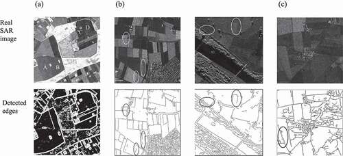
Figure 2. Examples of synthetic images of simulated simple scenarios. a) Wei and Feng (2015) b) Zhan et al. (2013) c) Xiang et al. (2017b).

Synthetically generated images provide ground-truth edge annotations so that the authors calibrate the parameters of their algorithms using quantitative evaluations. The parameters achieving the highest performance are selected and applied to real SAR images to provide qualitative evaluations. Nonetheless, the quantitative evaluations and the parameters selection process are based only on a couple of simple images, as presented in Figure 2. Therefore, the generalized performance of the proposed methods is not truly reflected as real-world patterns are much more complex and diverse. The main reason behind is the lack of large-scale datasets with ground-truth edge annotations. There also emerges another problem that a quantitative benchmark is missing in the field. Thus, at the moment, it is not possible to fully evaluate a (new or existing) method. Moreover, there is simply no fair way to compare the results to other research since the same evaluation images are not utilized and mostly a small number of comparison methods are evaluated. In that sense, Bachofer et al. (2016) provide the only work on the comparison of different combinations of speckle reduction techniques and optical edge detection methods. However, they evaluate four fundamental methods on only four images with multilooking. Thus, a comprehensive evaluation of the baseline methods is also missing in the field.

Therefore, in this paper, we aim to close all the aforementioned gaps. Recently, Liu et al. (2020) have simulated a large-scale SAR dataset called BSDS500-speckled exploiting an optical imagery dataset of natural scenes to train their CNN for edge detection in SAR images. The dataset is generated by multiplying the greyscale intensity optical images with a 1-look simulated speckle noise. Including different augmentations, the dataset includes $28,800$ training images and $200$ test images. Thus, instead of using a couple of simple synthetic images, we propose to use the training set of the BSDS500-speckled (28,800 images) for parameter tuning. The detectors with the best-performing parameters on the training set are eventually evaluated on the test set to form a benchmark. With this benchmark, we provide the most extensive experimental evaluation for SAR images on edge detection and thereby addressing the lack of large-scale experimental reviews in the remote-sensing field. The review also includes the performance evaluations of a number of denoising algorithms. To that end, we evaluate the following edge detectors: Roberts Cross, Prewitt, Sobel, Scharr, Farid, Frei-Chen, Laplacian of Gaussian (LoG), Differences of Gaussians (DoG), Canny, Gabor filters, a K-means clustering-based edge detector, a 2D wavelet discrete transformation-based edge detector, a subpixel edge detection algorithm based on partial area effect, Touzi, gradient by ratio (GR), Gaussian-Gamma-shaped (GSS) bi-windows, ratio of local statistics with robust inhibition augmented curvilinear operator (ROLSS RUSTICO), a SAR-specific Shearlet transformation-based edge detector, and the supervised CNN model of Liu et al. (2020). In addition, for the first time in literature, we explore a bundle of decision fusion methods for the task, which aims to combine the outputs of different algorithms. We hope that our work will serve as a baseline for future SAR-specific edge detection algorithms.

2. Related work

2.1. Denoising

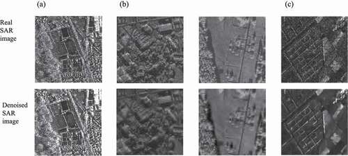
Noise is a random variation of pixel intensities arising from the acquisition process of the digital images. Among different noise patterns, speckle noise gets created because of random interference between the coherent returns due to the differences in the surface within pixels (Boncelet 2009). In that sense, unlike optical images, SAR images are highly corrupted with speckle noise. As a result, basic edge detection methods might produce unsatisfactory results for radar images (Touzi et al. 1988). The main problem is that the speckle noise patterns may be identified as false edges. Therefore, although SAR images are widely appreciated thanks to their high-resolution, wide-area coverage, and weather and illumination invariant properties, they also bring challenges. The speckle noise characteristics make them exceedingly challenging to process. To that end, denoising algorithms aim to decrease the amount of noise while preserving important structures. Thus, the task is an active area of research. A number of examples are presented in Figure 3.

Figure 3. A) Denoised with SAR-BM3D. Credits: (Parrilli et al. 2011). b) Denoised with soft thresholding. Credits: (Achim et al. 2003). c) Denoised with SAR-CNN. Credits: (Molini et al. 2020).

It is not possible to entirely denoise the speckled images (Singh and Shree 2016). Nevertheless, there are various techniques that aim to reduce the speckle. For instance, by combining statistically uncorrelated speckle patterns, multi-look images can be created. The disadvantage of this method is the decreased system resolution (Ouchi 1985). In this paper, we consider the more challenging 1-look images. In addition, most denoising algorithms only model additive noise, making them less fitting for the multiplicative speckle noise. A way to still use the additive denoising algorithms is to convert SAR images to the natural logarithm domain before applying the methods.

The two main categories for the denoising task are spatial and transform domain filtering. Linear and non-linear filters divide the former into two categories. The non-linear filters do not assume a distribution of the random noise. Transform domain filtering first transforms the noisy images and attempts to denoise the transformed image. Preserving image features, including edges and corners, is a major challenge in reducing noise (Jain and Tyagi 2016). Low-level denoising methods use only convolutions with hand-crafted filters. The median, mean and Gaussian are the most common filtering options and have the drawback of smearing out some of the true edges.

Here, we iterate over a number of methods that we utilize in our experiments. First of all, with Gaussian smoothing, a Gaussian (the normal distribution) is convolved over an image. It is a local operation that averages neighbourhoods according to a Gaussian distribution with a given standard deviation. The advantage of this filter is that blobs are preserved, while with a strong mean filter, blobs can blend together. It is among the most commonly used methods. In addition, Block-Matching and 3D Filtering (BM3D) is a block-matching algorithm proposed by Dabov et al. (2007). It takes a 2D block of an image and then finds similar blocks within the image. These similar blocks do not only have a similar average intensity but a comparable noise distribution. They are grouped into a 3D array. Then, the 3D arrays are processed with collaborative filtering. This grouping method reveals fine details while preserving important structures. Bilateral filtering is another smoothing method that preserves structures (Tomasi and Manduchi 1998). It takes the average of surrounding pixels, which generally becomes problematic at edges since they get averaged out. The variation of intensities is taken into account to prevent this. In addition, anisotropic diffusion takes the average of neighbourhoods, even if these neighbourhoods contain edges. It aims to only smooth out pixels on the same side of an edge, and thus it tends to generate appealing results on the supposedly homogeneous parts (Perona and Malik 1990). Finally, instead of just taking a local average with a small kernel, non-local means denoising (NLMD) considers the image as a whole. Then, the averages are weighted. Similar pixels get a higher weight than non-similar pixels. It tends to preserve edges and other details better than local denoising algorithms (Buades et al. 2005). On the other hand, more advanced methods utilize powerful deep-learning models (Zhang et al. 2017, 2018; Kim et al. 2019; Tian et al. 2020; Byun et al. 2021).

There also exists SAR-specific denoising methods. For example, SAR expansions of NLMD, BM3D, anisotropic diffusion, bilateral filtering are proposed (Gupta et al. 2013; D’Hondt et al. 2013; Zhao et al. 2014; Sica et al. 2018). Furthermore, supervised deep-learning methods tend to outperform classic methods. Lattari et al. (2019) present an encoder-decoder-based CNN for end-to-end denoising. In addition, Cozzolino et al. (2020) present a non-local filtering method powered by deep learning where the coefficients of the weighted average of neighbours are learned by a CNN. Moreover, Vitale et al. (2021) propose a CNN with a multi-objective loss function considering spatial and statistical properties of the SAR images. Nonetheless, these CNNs need annotated data to train on, which is not always available for real SAR images. To tackle this problem, recently, Molini et al. (2021) introduce a self-supervised Bayesian method with similar or better performance to the supervised training approaches. A detailed review on deep-learning techniques applied to SAR image denoising task and the recent trends can be found in the work of Fracastoro et al. (2021).

2.2. Benchmarks datasets

Benchmark datasets are of great importance for the development of machine-learning algorithms. They allow for fair evaluations and comparisons between different algorithms using quantitative evaluation metrics. They provide overviews about the algorithms’ ability to discover old and also new patterns, their superior sides and also limitations, time and space complexities, and thus their respective strengths and weaknesses. Hence, performances of algorithms against state-of-the-art or other competitive models can be assessed. One example is the famous MNIST dataset consisting of 60,000 training images and 10,000 testing images of 28 x 28 pixels with human annotated examples of handwritten digits (LeCun et al. 1998). Modern machine-learning algorithms already achieve around an accuracy of 99% in correctly classifying the digits. As a result, nowadays, it serves as a baseline as the first step for many classifiers to first test on; if the performance of the model is not decent, then there is little chance for it to work on more complex tasks.

Similarly, large-scale benchmark datasets have enabled computer vision research to make significant progress over the last years, especially with the rise of deep learning. The most famous example is the ImageNet project (Russakovsky et al. 2015), which is a benchmark in object category classification and detection, currently including more than 14 million images labelled into 20,000 different categories. The extraordinary performance of the revolutionary deep CNN architecture AlexNet (Krizhevsky et al. 2012) on the benchmark marks the beginning of the deep-learning era for computer vision. In parallel, many famous CNN models are emerged following the benchmark to beat AlexNet, such as VGGNet (Simonyan and Zisserman 2015), Inception (Szegedy et al. 2015), ResNet (He et al. 2016), DenseNet (Huang et al. 2017), Squeeze-and-Excitation (Hu et al. 2018) and EfficientNet (Tan and Le 2019). Other popular and large-scale computer vision datasets include CIFAR, Microsoft COCO, PASCAL VOC, Cityscapes and SUN (Krizhevsky 2009; Lin et al. 2014; Everingham et al. 2015; Cordts et al. 2016; Xiao et al. 2016). Thanks to their success on the real world large scale benchmarks, nowadays, CNNs are widely preferred, from face recognition to autonomous driving, in daily life where computer vision is utilized.

In addition, the large-scale benchmark datasets are widely utilized for transfer learning. Since it is not always possible to find or collect large-scale data sources for each problem or use case, models trained on large-scale benchmarks are assumed to learn generic features, such as edges and contours, that can be transferred to different domains. Likewise, instead of using random weights, pre-trained model weights can be used to initialize deep models to accelerate the learning process. Finally, large-scale benchmarks can be employed for self-supervised training of proxy tasks for smart model initialization, such as colorization or guessing the spatial configuration for two pairs of patches as proxy tasks for visual understanding (Larsson et al. 2017; Doersch et al. 2015). Similar techniques are also successfully applied to remote-sensing images (Tao et al. 2020; Stojnic and Risojevic 2021).

In parallel with the developments in digital instruments and big data, remote-sensing imagery becomes more and more widely available also introducing benchmark datasets to boost the development of new and improved algorithms. For instance, Yang and Newsam (2010) provide a 21 class land-use image set called UC Merced Land Use dataset, where each class has 100 images, for land-use classification in high-resolution overhead imagery. Additionally, Xia et al. (2018) produce a large-scale dataset for object detection in aerial images called DOTA, together with a challenge. It’s final version consists of 18 categories spanned into 11,000 images and around 1,800,000 instances. Similarly, Li et al. (2020) present DIOR, a large‐scale benchmark for object detection with around 23,000 images and 190,000 instances of 20 object classes. They also evaluate several state-of-the-art approaches to establish a baseline. Besides, PatternNet administers 38 different classes, having 800 images each, for remote-sensing image retrieval and also provide extensive evaluation of various methods to form a baseline (Zhou et al. 2018). Moreover, SpaceNet provide large-scale labelled satellite imagery and competitions for automated building footprint extraction and road network extraction for disaster management scenarios (van Etten et al. 2019). Likewise, xBD dataset provides before and after event satellite imagery for assessing building damage for disaster recovery research, together with a challenge (Gupta et al. 2019). Furthermore, FloodNet dataset provides high-resolution unmanned aerial vehicle imagery captured after Hurricane Harvey over Texas and Louisiana in August 2017 (Rahnemoonfar et al. 2021). It also provides two challenges; image classification and semantic segmentation, and visual question answering to boost the developments in the field. A review on benchmarking in photogrammetry and remote-sensing with an overview can be found in the work of Bakula et al. (2019). Finally, ImageNet benchmark has been successfully utilized for remote-sensing applications as well by transfer learning. For instance, Marmanis et al. (2015) use pretrained ImageNet features for classifying remote-sensing data that improves the overall accuracy from 83.1% up to 92.4% on the UC Merced Land Use benchmark. Similarly, Salberg (2015) utilizes generic image features extracted from AlexNet trained on the ImageNet database for automatic detection of seals in remote-sensing images. All in all, from the literature, it can be noticed that existing remote-sensing dataset are mainly limited to high level tasks such as classification or semantic segmentation.

As for SAR-specific datasets, So2Sat LCZ42 provides a benchmark for global local climate zones classification (Zhu et al. 2020), OpenSARUrban introduces a benchmark for urban scene classification together with extensive baseline evaluations (Zhao et al. 2020). They can be considered as general scene classification challenges. There also exists fine-grained object detection baselines for specific use cases such as ship detection (Huang et al. 2018; Wei et al. 2020). In addition, as part of the SpaceNet data corpus, MSAW presents dataset, baseline and challenge focusing on building footprint extraction (Shermeyer et al. 2020). Moreover, Sen1Floods11 introduces a georeferenced dataset to evaluate methods on flood detection. These can be considered as semantic segmentation benchmarks. On the other hand, there hardly exists datasets or benchmarks for low-level image processing tasks such as edge detection, noise reduction, contrast enhancement, image stitching or image sharpening. Therefore, a number of remote-sensing researchers have compiled their own individual reference data for the evaluations. Moreover, although methods might yield robust and effective results on their reference data, the comparisons tend to include only a couple of competitive approaches. Therefore, a comprehensive evaluation of the baseline methods is also missing in the field. Thus, in this paper, we aim to close the aforementioned gaps by providing extensive experimental evaluations for SAR images on the edge detection task to form the first benchmark and thereby addressing the lack of large-scale experimental reviews in the remote-sensing field.

3. Edge detection

One of the oldest operations in image processing and a building block for more complex algorithms is edge detection (Sponton and Cardelino 2015). Edges can give indications for boundaries and contours, and can help describe the (geometric) forms of objects in images. An edge reveals itself by an abrupt change in pixel intensity values. In that sense, for SAR images, an edge can be characterized by the boundary between two homogeneous regions such as the borders between two different croplands or the intersections between land and sea.

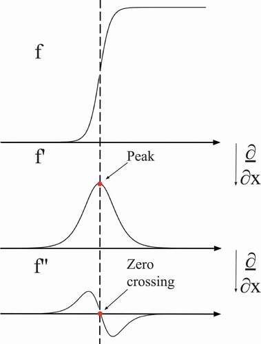
There are two main families of edge detection: first and second derivative based. The first derivative edge detection is the most commonly used. With the first derivative-based edge detection, an edge can be detected by a peak, whereas with the second derivative-based edge detection, it can be detected by a zero-crossing, see Figure 4. The computational costs of the methods that are based on the first derivatives (e.g. Sobel, Roberts Cross and Prewitt) are low compared to more complex edge operations. Thus, these detectors are at the bottom of the hierarchy, considered as low level and straightforward without any parameters to tune. The methods that are based on second derivatives usually include a smoothing step for noise reduction. Nonetheless, that also brings the challenge of selecting the optimum smoothing parameter. Thus, each edge detector has both advantages and disadvantages.

Figure 4. Difference in first and second derivatives-based edge detection. f indicates the image intensity.

3.1. First-order derivatives

Since edges are defined by an abrupt change in pixel intensity values, first-order derivatives search for the (local) maximum variations in the first derivatives of an image. The most common way to estimate the first derivative is by the first-order Taylor expansion with a small step as provided in Equations 1 and 2 as follows:

(1) $\mathrm{\Delta }x=\frac{\mathrm{\partial }f(x,y)}{\mathrm{\partial }x}=\frac{f(x+dx,y)-f(x,y)}{dx}.$(1)

(2) $\mathrm{\Delta }y=\frac{\mathrm{\partial }f(x,y)}{\mathrm{\partial }y}=\frac{f(x,y+dy)-f(x,y)}{dy}.$(2)

Since digital images are discrete, the small step can be considered as 1 (pixel), when $dx=1$, which leads to Equations 3 and 4, where $x$ and $y$ now denote pixel coordinates.

(3) $\mathrm{\Delta }x=\frac{\mathrm{\partial }f(x,y)}{\mathrm{\partial }x}=f(x+1,y)-f(x,y).$(3)

(4) $\mathrm{\Delta }y=\frac{\mathrm{\partial }f(x,y)}{\mathrm{\partial }y}=f(x,y+1)-f(x,y).$(4)

To compute the discrete derivatives (i.e. finite differences), simple 1D filters (kernels) can be utilized:

$Gx=\left[\begin{array}{cc}-1& 1\end{array}\right]$, $Gy=\left[\begin{array}{c}-1\\ 1\end{array}\right]$,

where $Gx$ and $Gy$ (convolutional) filters compute gradient responses in the horizontal and vertical directions. Then, the gradient magnitude ($G$) (the edge response map) per pixel is calculated by Equation 5 as follows:

(5) $G=\sqrt{G_x^2+G_y^2}.$(5)

The gradient magnitude points to the direction of the most significant change in intensity. Then, the orientation is computed by Equation 6 as follows:

(6) $\theta =ta{n}^{-1}\frac{G_y}{G_x}.$(6)

Once the gradient magnitude is computed, a threshold is set to decide from which pixels of the response map to be considered as true edges. Setting the threshold to lower values might capture unnecessary details (e.g. noise), whereas higher values might ignore critical structures. Thus, an optimum threshold is desired. The standard procedure of the first order derivatives-based edge detection is illustrated in Figure 5.

Figure 5. First order derivatives-based edge detection workflow.

Obviously, 1D differentiation filters do not consider diagonal edges. To achieve that 2D filters are required. The most commonly used 2D filters are Sobel, Roberts Cross and Prewitt operators (Duda and Hart 1973; Roberts 1963; Prewitt 1970).

3.1.1. Roberts cross

Instead of approximating gradients along the horizontal and vertical directions, diagonal directions can also be considered (i.e. 45${ }^{\circ }$ and 135${ }^{\circ }$). To that end, Roberts (1963) offers two kernels to compute the gradient magnitude:

$Gx=\left[\begin{array}{cc}1& 0\\ 0& -1\end{array}\right]$, $Gy=\left[\begin{array}{cc}0& 1\\ -1& 0\end{array}\right]$.

Therefore, it also generates high responses to changes in diagonal directions. It is mostly preferred for its simplicity. Nonetheless, its small kernels make it very sensitive to noise. Moreover, due to the coefficients of the filters, it can only capture sharp edges.

3.1.2. Prewitt

Different from the Roberts Cross filters, Prewitt (1970) offers 3 x 3 kernels to compute the gradient using eight directions:

$Gx=\left[\begin{array}{ccc}1& 0& -1\\ 1& 0& -1\\ 1& 0& -1\end{array}\right]$, $Gy=\left[\begin{array}{ccc}1& 1& 1\\ 0& 0& 0\\ -1& -1& -1\end{array}\right]$.

Similar to Roberts Cross, Prewitt is mostly preferred for its simplicity. Moreover, it provides some robustness to noise by differentiating in one direction and averaging in another due to its larger filter size. Nonetheless, due to its coefficients, it is mostly suited for images with high contrast.

3.1.3. Sobel

Sobel filters are also 3 x 3, but they are biased towards the centre pixel by giving significant weight to the centre coefficients of the kernels (Duda and Hart 1973):

$Gx=\left[\begin{array}{ccc}-1& 0& 1\\ -2& 0& 2\\ -1& 0& 1\end{array}\right]$, $Gy=\left[\begin{array}{ccc}-1& -2& -1\\ 0& 0& 0\\ 1& 2& 1\end{array}\right]$.

Therefore, averaging gives more weight to central pixel, which results in smoother responses than Prewitt. Similar to Prewitt, it computes edges in eight directions. In addition, the filters are separable such that they can be expressed as a matrix product of a 1D column and a 1D row vectors, which can be utilized for faster computations.

3.1.4. Scharr

Scharr filters are very similar to Sobel, but with different coefficients. Nonetheless, unlike Sobel, Scharr provides anisotropic filters that tends to achieve better rotation invariance. The weights are derived by optimizing the weighted mean-squared angular error in Fourier domain (Scharr 2000):

$Gx=\left[\begin{array}{ccc}3& 0& -3\\ 10& 0& -10\\ 3& 0& -3\end{array}\right]$, $Gy=\left[\begin{array}{ccc}3& 10& 3\\ 0& 0& 0\\ -3& -10& -3\end{array}\right]$.

3.1.5. Farid

Similar to Scharr, Farid determines the filter weights by the optimization of the rotation invariance of the gradient operator in the Fourier domain (Farid and Simoncelli 2004):

$Gx=\left[\begin{array}{ccccc}0.004128& 0.027308& 0.046732& 0.027308& 0.004128\\ 0.010420& 0.068939& 0.117974& 0.068939& 0.010420\\ 0.0& 0.0& 0.0& 0.0& 0.0\\ -0.010420& -0.068939& -0.117974& -0.068939& -0.010420\\ -0.004128& -0.027308& -0.046732& -0.027308& -0.004128\end{array}\right],$

$Gy=\left[\begin{array}{ccccc}0.004128& 0.010420& 0.0& -0.010420& -0.004128\\ 0.027308& 0.068939& 0.0& -0.068939& -0.027308\\ 0.046732& 0.117974& 0.0& -0.117974& -0.046732\\ 0.027308& 0.068939& 0.0& -0.068939& -0.027308\\ 0.004128& 0.010420& 0.0& -0.010420& -0.004128\end{array}\right].$

Different from the previous filters, Farid’s coefficients are of float data type which makes it computationally more expensive. Note that we round the weights to 6 decimals for better presentation. Additional decimal places can be found in Python’s scikit-image package.¹ Furthermore, Farid’s smallest filter size is 5 x 5 which is again computationally more demanding than the previous filters. Nonetheless, larger mask size might be beneficial in reducing the the effects of noise by local averaging within the neighbourhood, yet it might also cause more blurring. As a final remark, extended versions (i.e 5 x 5 or 7 x 7) of the aforementioned filters also exist (Lateef 2008; Kekre and Gharge 2010; Bogdan et al. 2020), yet we respect the original algorithms and use them without any extensions.

3.1.6. Frei-Chen

Different from the previous methods which provide horizontal and vertical filters, Frei-Chen method offers nine kernels that contain all of the basis vectors so that the local neighbourhood (i.e 3 x 3) is represented by the weighted sum of those nine basis vectors (Frei and Chen 1977):

$w_1=\left[\begin{array}{ccc}1& \sqrt{2}& 1\\ 0& 0& 0\\ -1& -\sqrt{2}& -1\end{array}\right]$, $w_2=\left[\begin{array}{ccc}1& 0& -1\\ \sqrt{2}& 0& -\sqrt{2}\\ 1& 0& -1\end{array}\right]$, $w3=\left[\begin{array}{ccc}0& -1& \sqrt{2}\\ 1& 0& -1\\ -\sqrt{2}& 1& 0\end{array}\right]$,

$w4=\left[\begin{array}{ccc}\sqrt{2}& -1& 0\\ -1& 0& 1\\ 0& 1& -\sqrt{2}\end{array}\right]$, $w5=\left[\begin{array}{ccc}0& 1& 0\\ -1& 0& -1\\ 0& 1& 0\end{array}\right]$, $w6=\left[\begin{array}{ccc}-1& 0& 1\\ 0& 0& 0\\ 1& 0& -1\end{array}\right]$,

$w7=\left[\begin{array}{ccc}1& -2& 1\\ -2& 4& -2\\ 1& -2& 1\end{array}\right]$, $w8=\left[\begin{array}{ccc}-2& 1& -2\\ 1& 4& 1\\ -2& 1& -2\end{array}\right]$, $w9=\left[\begin{array}{ccc}1& 1& 1\\ 1& 1& 1\\ 1& 1& 1\end{array}\right]$.

Filters $w1$, $w2$, $w3$ and $w4$ capture the edge subspace, $w5$, $w6$, $w7$ and $w8$ capture the line subspace, and $w9$ captures the average subspace. It is computationally more expensive than the previous methods utilizing 3 x 3 kernels as it has seven more kernels and a number of them with float data type coefficients. We exclude the averaging operation $w9$ as it does not include derivatives and combine all the responses ($w1$, … , $w8$) as done in Equation 5.

3.2. Second-order derivatives

It is also possible to reveal edges by exploiting the second-order derivatives by detecting zero crossings. First-order derivatives search for the peaks that are above a certain threshold, whereas the second-order derivatives automatically identify the local maxima. Nonetheless, the first-order derivatives are more robust to noise than the second-order derivatives as further differentiation amplifies the noise. The most commonly used second-order derivative operations are Laplacian of Gaussian (LoG) and Difference of Gaussians (DoG) (Marr and Hildreth 1980).

3.2.1. Laplacian

One way to calculate the second derivative of an image is computing the Laplacian. Since the Laplacian is the divergence of a gradient, it can represent the second derivative by highlighting rapid intensity changes. Similar to the first-order derivatives (in Equations 1, 2, 3 and 4), it can be represented as follows:

(7) ${\mathrm{\Delta }}^{2}f=\frac{{\mathrm{\partial }}^{2}f}{\mathrm{\partial }{x}^2}+\frac{{\mathrm{\partial }}^{2}f}{\mathrm{\partial }{y}^2}.$(7)

(8) ${\mathrm{\Delta }}^{2}x=\frac{{\mathrm{\partial }}^{2}f}{\mathrm{\partial }{x}^2}=f(x+1,y)+f(x-1,y)-2f(x,y).$(8)

(9) ${\mathrm{\Delta }}^{2}y=\frac{{\mathrm{\partial }}^{2}f}{\mathrm{\partial }{y}^2}=f(x,y+1)+f(x,y-1)-2f(x,y).$(9)

For an additional comparison between the first and second derivative filters, see Figure 6. To approximate the effect of the Laplacian, the following 3 x 3 discrete convolution kernel can be utilized by adding the vertical and horizontal derivative filters in Figure 6:

Figure 6. Examples of directional filters. α is measured counterclockwise from the horizontal axis. Credits: Schowengerdt (2007).

$\mathcal{L}=\left[\begin{array}{ccc}0& 1& 0\\ 1& -4& 1\\ 0& 1& 0\end{array}\right].$

Note that since the Laplacian utilizes a single mask, the edge orientation information is not available. Finally, the Laplacian operator usually is not used individually as it is more sensitive to noise than the first-order based methods due to the additional differentiation. Thus, it is a common practice to combine it with a smoothing operation.

3.2.2. Laplacian of Gaussian (LoG)

The LoG is an extension to the Laplacian filter, where the Laplace response is combined with a Gaussian filter. The Laplacian is good at detecting thin edges, but it is more sensitive to noise than the first derivative variants. To keep the false detection of edges to a minimum, a Gaussian filter is applied to an image, before detecting the edges with a Laplacian convolution. Nonetheless, the smoothing might smear out some of the sharp edges lowering the precision in edge localization. Thus, the smoothing parameter should be treated carefully. Finally, the thresholding is achieved by zero-crossing, which is the key feature of this algorithm. To that end, the Gaussian kernel is estimated by Equation 10, then taking the Laplacian of the Gaussian equation by Equation 11, LoG filter is realized in Equation 12 as follows:

(10) $G(x,y;\sigma )=\frac{1}{2\pi {\sigma }^2}exp(\frac{-x^2-y^2}{2{\sigma }^2}).$(10)

(11) ${\mathrm{\Delta }}^2(G(x,y;\sigma ))=\frac{{\mathrm{\partial }}^2}{\mathrm{\partial }{x}^2}G(x,y;\sigma )+\frac{{\mathrm{\partial }}^2}{\mathrm{\partial }{y}^2}G(x,y;\sigma ).$(11)

(12) $LoG={\mathrm{\Delta }}^2(G(x,y;\sigma ))=\frac{1}{\pi {\sigma }^4}(\frac{x^2+y^2}{2{\sigma }^2}-1)exp(\frac{-x^2-y^2}{2{\sigma }^2}),$(12)

where $\sigma$ denotes the standard deviation of the Gaussian.

3.2.3. Difference of Gaussians (DoG)

The DoG takes two Gaussians with different variances of an image and calculates the difference. Edges are identified by the differences of the convolutions of the two Gaussian kernels with the image as follows:

(13) $DoG=G_{{\sigma }_1}-G_{{\sigma }_2}=\frac{1}{\sqrt{2\pi }}(\frac{1}{{\sigma }_1}exp(\frac{-x^2-y^2}{2{\sigma }_1^2})-\frac{1}{{\sigma }_2}exp(\frac{-x^2-y^2}{2{\sigma }_2^2})),$(13)

where ${\sigma }_1$ and ${\sigma }_2$ represent the two standard deviations of the Gaussian. Before taking the differences, each Gaussian function is normalized so that the area under the curve is one, making the mean difference is zero. It basically subtracts a highly smoothed version of an image from the less smoothed one, acting as a band-pass filter ignoring high-frequency components that are often attributed to noise. Finally, the thresholding is achieved by zero-crossing, similar to LoG. Additionally, with particular parameter settings DoG becomes an approximation of the LoG. In terms of the computational complexity, there is no significant difference between these two approaches.

3.3. Advanced methods

In addition to the commonly used first- and second-order derivative-based filters, we also iterate over a number of advanced methods that use additional features or steps in their algorithms.

3.3.1. Canny

Canny is one of the most widely used edge detection algorithms (Canny 1986). It is composed of noise reduction, gradient calculation, non-maximum suppression, double thresholding and hysteresis. Firstly, it smooths an image with a Gaussian kernel. Secondly, the response is convolved with a low-level edge detector (e.g. Sobel or Roberts) to obtain the gradient image. Afterwards, non-maximum suppression is applied to extract thin edges by identifying the pixel with the maximum value in an edge. Then, by setting a high and a low threshold, strong and weak edges are determined. The strong edge pixels are labelled as final edges. In the ultimate stage, hysteresis decides which of the weak edges are considered as true edges by tracking the edge connections within a neighbourhood. Non-maximum suppression and hysteresis steps greatly contribute to reducing the number of false edges. Nonetheless, these steps also increase the computation time. Finally, the algorithm has three main parameters to tune (sigma for Gaussian smoothing and two thresholds), which makes it more demanding than the previously mentioned methods.

3.3.2. Gabor filters

Gabor filters are mostly used for texture analysis and feature extraction as they have been shown to have optimal localization both in spatial and frequency domains (Daugman 1985). Similar to DoG, Gabor filters act as adjustable band-pass filters. A Gabor function is a Gaussian function modulated with a complex sinusoidal carrier signal. To extract features of different shapes, orientations, and scales, it is common practice to combine multiple filters together in a filter-bank, as illustrated in Figure 7. This is similar to the case of Frei-Chen where different kernels are constructed to capture different patterns. Nonetheless, Gabor filters can be created with an endless amount of orientations, combinations, and smoothing settings. A 2D Gabor function contains real and imaginary parts as described in Equations 14(14) $g(x,y;\lambda ,\theta ,\sigma ,\gamma {)}_{real}=exp(\frac{-x^2-{\gamma }^2{y}^2}{2{\sigma }^2})cos(\frac{2\pi x}{\lambda }+\phi )),$(14) and 15(15) $g(x,y;\lambda ,\theta ,\sigma ,\gamma {)}_{imaginary}=exp(\frac{-x^2-{\gamma }^2{y}^2}{2{\sigma }^2})sin(\frac{2\pi x}{\lambda }+\phi )),$(15) :

Figure 7. Example of the real parts of the Gabor filters with different orientations and frequencies to capture various patterns. These filters are also used to create one of our filter banks.

(14) $g(x,y;\lambda ,\theta ,\sigma ,\gamma {)}_{real}=exp(\frac{-x^2-{\gamma }^2{y}^2}{2{\sigma }^2})cos(\frac{2\pi x}{\lambda }+\phi )),$(14)

(15) $g(x,y;\lambda ,\theta ,\sigma ,\gamma {)}_{imaginary}=exp(\frac{-x^2-{\gamma }^2{y}^2}{2{\sigma }^2})sin(\frac{2\pi x}{\lambda }+\phi )),$(15)

where for the spatial location $(x,y)=(xcos\theta +ysin\theta ,-xsin\theta +ycos\theta )$, $\lambda$ and $\phi$ denote the wavelength and the phase offset of the sinusoidal carrier signal, $\theta$ controls the orientation, and $\sigma$ and $\gamma$ indicate the standard deviation and the spatial aspect ratio of the Gaussian. Finally, the response of each convolution with a real and imaginary Gabor kernel is combined by accumulating the real and imaginary parts as follows:

(16) $R=\sqrt{{(I\ast g_{i_{real}})}^2+{(I\ast g_{i_{imaginary}})}^2},$(16)

where $g$ indicates a Gabor kernel. To create a filter bank, various Gabor kernels are created with different orientations and frequencies. Then, the response ($R$) of each kernel can be combined together by summing them to create a superimposed edge response map (gradient magnitude). Other options might include taking the maximum response per pixel or simply computing the average responses over all kernels.

3.3.3. K-means clustering

K-means clustering algorithm can also be utilized to split an image into a number of clusters based on pixel intensities to detect different regions. The number is of clusters is defined by the hyperparameter $K$. It can be particularly useful as the derivatives-based edge detection methods using filters are known to be sensitive to noise as they operate over small neighbourhoods. On the other hand, when an image is grouped into a small number of regions, the boundaries between the clusters are expected to reveal true edges. For example, given an image containing only water and land pixels, and using $K=2$, the algorithm is to divide those pixel values in two distinct clusters. Then, applying a low-level edge detector (e.g. Sobel), the boundaries between the clusters can be extracted as edges. It is a suitable option for SAR images since the edges often manifest as boundaries between homogeneous areas.

3.3.4. 2D discrete wavelet transformation

A wavelet transformation decomposes image signals to different scales of frequency bands, which may be considered isotropic low-pass and high-pass components (Schowengerdt 2007). One level decomposition provides four different sub-bands namely low-low (LL), low-high (LH), high-low (HL) and high-high (HH). Using these four sub-bands, the original image can be reconstructed. The LL sub-band is composed of an approximation of the original image and it can be decomposed further, while the rest of the components are composed of the high-frequency information that are expected to highlight edges. Firstly, we apply the 2D discrete wavelet transformation using a biorthogonal wavelet. Then, the LL component is discarded as it does not contain high-frequency information and the rest of the components are combined into an edge response map similar to the previous cases as follows:

(17) $\mathrm{D}\mathrm{W}\mathrm{T}=\sqrt{\mathrm{L}{\mathrm{H}}^2+\mathrm{H}{\mathrm{L}}^2+\mathrm{H}{\mathrm{H}}^2}.$(17)

3.3.5. Subpixel edge detection

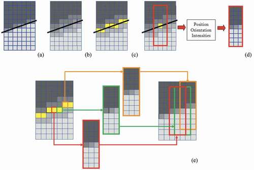
Figure 8 illustrates the difference between the subpixel edge detection and the derivatives-based methods. Since the derivatives-based edge detection methods operate on the the discrete structure of the digital images, they characterize a pixel into a single region. Nonetheless, object shapes may be projected with inaccuracies or unambiguously registered during the image acquisition process which might affect the true position of an edge pixel. To address these issues, subpixel methods aim at recognizing the location and orientation of an edge within a pixel with high precision. To that end, Trujillo-Pino et al. (2013) propose a subpixel edge detection algorithm based on partial area effect, which assumes a particular discontinuity in the edge location and that pixel values are proportional to the intensities and areas at both sides of an edge. It first applies a 3 x 3 averaging filter to smooth the input image. Then, the partial derivatives of the smoothed image are computed. Afterwards, a 9 x 3 window is centred on the each pixel of the partial derivatives to ensure that an edge crosses the window from left to right. Later, the sum of the right, middle and left column of the window are computed to solve three system of linear equations to obtain the edge features; orientation, curvature and change in intensity in both sides of the edge. Finally, the subpixel position is calculated by measuring the vertical distance from the centre of the pixel to the edge. Edges are detected by a threshold that considers a minimum intensity change. If a pixel is marked as an edge by the algorithm, a restored subimage is generated containing a perfect edge. The process is applied for each pixel position and the generated subimages are combined to achieve one final edge map. The whole procedure can be repeated to refine the results of a previous iteration. It is illustrated in Figure 9. We refer the reader to the work of Trujillo-Pino et al. (2013) for mathematical derivations and additional details.

Figure 8. Subpixel edge detection where edges are precisely located inside the pixels. Credits: (Trujillo-Pino et al. 2013).

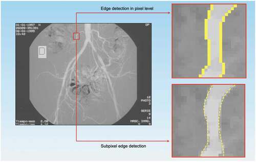
Figure 9. Subpixel edge detection algorithm based on partial area effect. a) Input image; b) Smoothed image; c) Detecting edge pixels; d) a synthetic 9×3 subimage is created from the features of each edge pixel; e) Subimages are combined to achieve a complete restored image. Credits: (Trujillo-Pino et al. 2013).

3.4. SAR-specific methods

In addition to the traditional optical methods, we analyse eight more edge detectors that are specifically tailored for SAR images; Touzi, gradient by ratio (GR), Gaussian-Gamma-shaped (GSS) bi-windows, ratio of local statistics with robust inhibition augmented curvilinear operator (ROLSS RUSTICO), a SAR-specific Shearlet transformation-based edge detector, GRHED - the supervised CNN model of Liu et al. (2020), and two different fusions of ($i$) the ratio of the averages (ROA) and the ratio of exponentially weighted averages (ROEWA)-based methods, and ($ii$) an optical and a SAR-specific method. These methods are designed to better handle the possible false edge artefacts due to the speckle noise.

3.4.1. Touzi

Touzi is a CFAR-based edge detector using the ratio of pixel values. It is designed to be more stable against the multiplicative speckle noise than the traditional edge detectors (Touzi et al. 1988). Therefore, instead of using differentiation, as in the case of first-order derivatives, it uses the ratio of the averages (ROA) of patches as the rate of false alarms is independent of the average local radiometry. 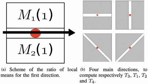It is computed for the four principal directions (0${ }^{\circ }$, 45${ }^{\circ }$, 90${ }^{\circ }$, 135${ }^{\circ }$) to capture horizontal, vertical and diagonal edges as the ratio of the means of the two neighbourhoods on the opposite sides of a pixel along a direction:

(18) $r=1-min\{\frac{{\mu }_1}{{\mu }_2},\frac{{\mu }_2}{{\mu }_1}\},$(18)

where μs are the arithmetic mean values of the two halves of a given window. At a given pixel, $r$ is calculated for the given directions and the maximum response corresponds to the edge response of that pixel. Finally, thresholding decides which pixels are true edges. The framework of computing the ratios is also demonstrated in Figure 10.

Figure 10. Scheme of the ROA method. Credits: Dellinger et al. (2015).

3.4.2. Gradient by ratio (GR)

Gradient by ratio method defines the horizontal and vertical gradient components as follows (Dellinger et al. 2015):

(19) $\begin{array}{c}{G}_{h,\alpha }=log(R_{h,\alpha }),\\ G_{v,\alpha }=log(R_{v,\alpha }),\end{array}$(19)

where Rs are the ratio of exponentially weighted averages (ROEWA) of the two halves of a given window. Different from the Touzi operator that uses straightforward averages, GR exponentially weights the average values by $\alpha$, which also controls the smoothing of the image at different scales. Finally, the gradient magnitude is calculated similar to the previous cases as the root mean square of the directional gradients:

(20) $G{R}_{\alpha }=\sqrt{{(G_{h,\alpha })}^2+{(G_{v,\alpha })}^2}.$(20)

3.4.3. Gaussian-Gamma-shaped (GSS) bi-windows

Different from the methods that use traditional rectangular bi-windows to compute the local statistics (e.g. Touzi), Shui and Cheng (2012) propose to utilize Gaussian-Gamma-shaped (GGS) bi-windows in ratio-based edge detectors to reduce the number of false edge pixels near true edges. Moreover, it provides flexible parameter selection, dynamic spacing between two windows to capture better curvilinear structures, and favourable smoothness in local statistics estimations. A comparison is presented in Figure 11. The authors demonstrate that the rectangle window functions are not reliable 2-D smoothing filters causing false edges around the proximity of true edges due to the remaining unwanted high-frequency speckle noise residuals. To overcome the problem of detecting false edges from false local maxima, GGS bi-windows are utilized for the horizontal components as follows:

Figure 11. Difference between (a) rectangle bi-windows and (b) GGS bi-windows at orientation ^π . Credits: Shui and Cheng (2012).

(21) $\begin{array}{c}W(x,y)=\frac{|y{|}^{\alpha -1}}{\sqrt{2\pi }{\sigma }_x\mathrm{\Gamma }(\alpha ){\beta }^{\alpha }}exp(-(\frac{x^2}{2{\sigma }_x^2}+\frac{|y|}{\beta })),\\ \hspace{0.17em}\end{array}$(21)

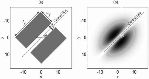
where $\sigma$ controls the window length, $\alpha$ controls the window width, $\beta$ controls the spacing of the two windows, and $(x,y)$ denotes pixel locations. The window is Gaussian shaped at horizontal and Gamma shaped at vertical orientation. Then, for each pixel and an orientation, the ratios of the local means in the GGS bi-windows are calculated.

3.4.4. Ratio of local statistics based on RUSTICO

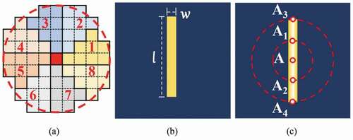
In order to make full use of the statistical characteristics of SAR images for the edge detection task, Li et al. (2022) introduce a method based on the ratio of local statistics (ROLSS) that is combined with the robust inhibition-augmented curvilinear operator (RUSTICO) which is inspired by the push-pull inhibition in visual cortex differentiating contrast variations (Strisciuglio et al. 2019b). It is recognized for its high robustness to noise and texture for the edge detection task. To compute an initial edge map, the method first utilizes an unweighted circle-shaped window to extract the ratio of local statistics (i.e. maximums of mean and standard deviation, similar to Equation 18):

(22) $E=R_1\times R_2,$(22)

where $R_1$ and $R_2$ are computed by the statistical ratios over the circle-shape window and defined as follows:

(23) $\begin{array}{c}{R}_1=max(R_{mean},\frac{1}{R_{mean}}),\\ \hspace{0.17em}\\ R_2=max(R_{std},\frac{1}{R_{std}}).\end{array}$(23)

Then, the edge response map, $E$, is augmented with RUSTICO by detecting the contrast variations using a DoG filter for noise robust curvilinear structure detection. Given a prototype pattern (e.g. a synthetic bar) and a reference point, it is computed by considering the positions of the local DoG maxima around a number of concentric circles positioned to the reference point, as illustrated in Figure 12.

Figure 12. (a) Circular window with 4 pixel radius, (b) prototype pattern (bar) for RUSTICO, (c) positions of local differences of the Gaussians’ maxima along with concentric circles. Credits: Li et al. (2022).

3.4.5. SAR-Shearlet

The standard wavelet transformations for the edge detection task are not robust to noise. Moreover, they tend to have difficulty in distinguishing close edges and have poor angular accuracy due to their isotropic nature. To address these limitations, shearlet transform is proposed, which is highly anisotropic, and defined at diverse scales, locations and orientations (Yi et al. 2009). It utilizes an anisotropic directional multiscale transform which produces a directional scale-space decomposition of images. In simple terms, given an image $I$, it is a mapping defined as follows:

(24) $I\to f_{\psi }I(\alpha ,s,p),$(24)

where $\alpha$ denotes the scale, $s$ denotes the orientation, $p$ denotes the pixel location, $\psi$ is the generating function of well-localized waveforms which is anisotropically scaled and sheared, and $f$ denotes the shearlet transform (Labate et al. 2005). Furthermore, the idea is extended for SAR images for bankline detection, which can be considered as curvilinear structures, and also for edge detection achieving promising results (Sun et al. 2021, 2022). To achieve that, complex shearlet transform is utilized as follows:

(25) $\psi ={\psi }^{even}+i{\psi }^{odd}={\psi }^{even}+iH({\psi }^{even}),$(25)

where ${\psi }^{even}$ denotes an even symmetric shearlet, ${\psi }^{odd}$ denotes an odd symmetric shearlet, and $H(.)$ denotes the Hilbert transformation. After applying complex shearlet transform to an image, the largest absolute value among all the coefficients related to the odd symmetric shearlet is determined and the corresponding shearlet direction is set as the main direction of the edge at a pixel. Using this principle direction, the even symmetric shearlet coefficient of the image is computed. Finally, the probability of a pixel being an edge is calculated at the main direction per pixel as follows:

(26) $\tilde{E}=\frac{|{\sum }_{J_{min}}^{J_{max}}<I,{\psi }^{odd}>|-{\sum }_{J_{min}}^{J_{max}}|<I,{\psi }^{even}>|}{(J_{max}-J_{min}+1)\times ma{x}_{j\in \{J_{min},\dots ,J_{max}}\}|<I,{\psi }^{odd}>|},$(26)

where $<.>$ denotes the related shearlet coefficients and $j$ is the scale parameter. We refer the reader to the works of Sun et al. (2021, 2022) and Reisenhofer et al. (2016) for additional details and derivations.

3.4.6. GRHED

GRHED is a convolutional neural network (CNN)-based edge detector for 1-look SAR images (Liu et al. 2020). It utilizes the Holistically Nested Edge Detection (HED) (Xie and Tu 2015) model together with a special hand-crafted layer. HED is a CNN-based end-to-end deeply supervised edge detection framework. It is designed to learn rich hierarchical features by progressively refining edge maps produced as side outputs using multi-scale learning. The final output is a weighted fusion of those side outputs. The framework adopts the commonly used VGGNet model with special modifications for the task at hand. We refer the reader to the original work of Xie and Tu (2015) for detailed model architecture, parameters and training choices.

Since HED model is designed for optical images, it is not directly suitable for the SAR image edge detection task as illustrated by Liu et al. (2020). It has problems with the speckle noise characteristics, different texture patterns and bright homogeneous regions. To address these issues, (Liu et al. 2020) add a hand-crafted layer before the learnable layers of HED. To that end, GR is utilized as the hand-crafted layer that generates gradient future maps which are not affected by the different intensity values and only depend on on the ratio of the mean values. Thus, the model first takes input as a 1-look SAR image, then it process the image with GR to extract gradient features. Finally, the gradient features are processed with a set of learnable convolutional layers to generate a final output containing the predicted edges of the 1-look SAR input.

The model is trained in a supervised fashion using the cross entropy loss utilizing a large-scale dataset by simulating SAR-like noise over the optical BSDS500 dataset (Arbelaez et al. 2011). We will use the same dataset for our parameter selection process and benchmark experiments, which is to be explained later in Section 4.

3.4.7. Fusion

Finally, we explore the effect of fusion over the performance. The motivation is that each edge detector has both advantages and disadvantages and we want to combine the advantages of different features while also mitigating the possible disadvantages. To that end, we combine ($i$) SAR-specific Touzi and the best-performing optical method, Farid, and ($ii$) ROA-based Touzi and ROEWA-based GR ($a$) by directly combining the normalized gradient magnitudes (edge responses), and ($b$) by combining thresholded normalized gradient magnitudes using a voting scheme. In that sense, for the first time in literature, we explore a bundle of decision fusion methods for the task. Surprisingly, the effect of fusion for combining two different SAR-specific edge detectors has never been explored before.

4. Experimental setup

For the experiments, following the setup of Liu et al. (2020) as a guideline, we utilize a large-scale dataset by simulating SAR-like noise over the optical BSDS500 dataset (Arbelaez et al. 2011). Then, four different denoising algorithms are applied to the entire dataset as a pre-processing step to achieve the cleanest image set. Afterwards, we utilize a variety of edge detection methods on the best-denoised images. Finally, by iterating over a set of thresholds and various hyperparameters, we evaluate the performances of the edge detectors and establish a benchmark for future evaluations.

4.1. Approach

The fundamental scheme for the edge detection task is demonstrated in Figure 13. The idea is to first smooth images to reduce the effect of noise, then enhance (identify) important features or details by gradient magnitude computation. Later, a threshold is applied to identify true edges (edge detection). An extra localization step can also be applied by edge thinning and linking to achieve one pixel wide continuous edges (e.g. Canny). If an extra localization step is not already a part of an algorithm, we do not include it. For example, Sobel does not have a localization step, whereas Canny inherently includes one. For our approach, smoothing is achieved by a set of denoising algorithms that are to be elaborated in Section 4.3. Then, for the enhancement step, each edge detection method has a way of calculating the gradient magnitude as provided in Section 3. Finally, for the detection step, we sample 20 threshold values and search for the value that achieves the best F1-score performance and also report a set of quantitative evaluation metrics for additional insights.

Figure 13. Fundamental edge detection steps.

4.2. Dataset

The original Berkeley Segmentation Data Set 500 (BSDS500) contains 500 natural optical images, among which 300 images are reserved for training and validating (from now on they will be referred as the training set), and 200 images are for testing (Arbelaez et al. 2011). It is widely used for contour and edge detection tasks for optical images as a benchmark. Ground truth edge maps are manually generated by human annotators. The number of annotations differs per image, yet each has five different annotations on average. Following the common practice, we consider any annotated pixel as ground truth for our evaluations, which results in edges that can sometimes be wider than one pixel, see Figure 14.

Figure 14. Sample images from the BSDS500-speckled dataset.

Using the training set of BSDS500, Liu et al. (2020) generate 1-look speckled data by multiplying the images by speckle noise patterns following the widely used Goodman model (Goodman 1975). The training set is further augmented by rotating images by 16 different angles, flipping horizontally, and rescaling to 50%, 100% and 150% of their original sizes. The resulting speckled optical dataset, named BSDS500-speckled, contains 28,800 images for training, and 200 images for testing and benchmarking. A number of images are presented in Figure 14. Using this dataset, Liu et al. (2020)train their supervised CNN model for edge detection on SAR images and achieve better results than the gradient by ratio method.

4.3. Denoising

The current literature bases the quantitative evaluations and the parameters’ selection process on a couple simple images, as provided in Figure 2. As a result, the generalized performance of the proposed methods is not truly reflected as real-world patterns are much more complex and diverse. The main reason behind has been the lack of large-scale datasets with ground-truth edge annotations. Thus, instead of using a couple of simple synthetic images, we propose to use the training set of the real-world BSDS500-speckled (28,800 images) for parameter tuning. The detectors with the best-performing parameters on the training set are eventually evaluated on the test set to form a benchmark. With this benchmark, we provide the most extensive experimental evaluation for SAR images on edge detection and thereby addressing the lack of large-scale experimental reviews in the remote-sensing field. We believe that our work will serve as a baseline for future SAR-specific edge detection algorithms by providing fair experimental evaluation. The dataset and the benchmark are available at https://github.com/readmees/SAR_edge_benchmark.git.

When using denoising as a pre-processing step for the edge detection task, there is a trade-off to consider. The more noise gets removed, the more (micro-)edges disappear so that some of the true edges are also smeared out. Therefore, we consider denoising algorithms that tend to preserve structures better. To that end, block-matching and 3D filtering (BM3D) (Makinen et al. 2020), bilateral filtering, anisotropic diffusion and non-local means denoising (NLMD) are to be evaluated. We use a bilateral filtering algorithm designed specifically for SAR (SARBLF) (D’Hondt et al. 2013). Both SARBLF and anisotropic diffusion are iterative algorithms. Thus, the noise (and with it micro-edges) is expected to be smoothed out more for higher number of iterations.

All the denoising algorithms are implemented in Python. BM3D implementation is taken from the original repository.² SAR-BM3D proposed by Parrilli et al. (2012) provides a SAR version of the algorithm based on a (2007) BM3D implementation. In their work, they state that the homomorphic BM3D performs quite similar. Thus, we assume the current improved version (2020) of BM3D is also sufficient for SAR images. Additionally, we use the OpenCV implementation of NLMD (Bradski 2000), and anisotropic diffusion by MedPy library.³ Finally, SARBLF is also taken from the original repository provided by its authors.⁴

All the denoising algorithms use their default settings unless stated otherwise. For BM3D and NLMD, the standard deviation of the noise is assumed to be 0.5 for all experiments. For anisotropic diffusion and SARBLF, we experiment with different number of iterations. Moreover, SARBLF has two parameters; spatial scale parameter (gs) to adjust the spatial extent of the filter, similar to the window size, and radiometric scale parameter (gr) to control the amount of filtering for weighting the local averages of intensities. The code provided by the authors use $gs=2.8$ and $gr=1.4$, whereas in their article, they use $gs=2.2$ and $gr=1.33$. Thus, we evaluate both settings. Finally, for the algorithms assuming additive noise, images are transformed to $log$ domain to also transform multiplicative speckle noise to additive noise.

For quantitative assessments, denoised images are compared against the clean images without any speckle (ground truth). To that end, the whole dataset of 29,000 images is evaluated using mean squared error (MSE) measuring per pixel reconstruction quality, peak signal-to-noise ratio (PSNR) measuring the noise difference in ratios, and structural similarity index (SSIM) measuring the similarity considering the perception of the human visual system. Both MSE and SSIM are in the range of $[0.0,1.0]$. For MSE, 0.0 indicates that the predictions perfectly match the ground-truths, thus the lower the better. On the other hand, for SSIM, 1.0 indicates a perfect match, thus the higher the better. Similarly, higher PSNR values indicate better reconstruction qualities. It is in the range of $[0.0,\mathrm{\infty })$. As a reference, SAR-BM3D achieves around 25.66 dB on its simulated speckle experiments.

4.4. Edge detection

For the methods that have parameters, the training set of 28,800 (denoised) images are utilized for parameter tuning. Then, the best-performing set of parameters are used to evaluate the test set of (denoised) 200 images to form the benchmark. For quantitative evaluations, we use the receiver operating characteristic (ROC) curve and its area under the curve (AUC) together with the metrics derived from confusion matrices. This metrics are precision (PPV), accuracy (ACC), F1-score (F1), and the Fowlkes–Mallows index (FM). For these metrics achieving 1 means the highest possible performance, while 0 indicates the lowest.

The ROC curve presents the change in true-positive rate (sensitivity or recall) against the false-positive rate (fall-out) by varying the threshold values. The perfect classification with no false negatives and no false positives generates a point in the upper left corner of the graph, whereas a random classification generates points along the diagonal line. Given that scheme, points above the diagonal indicate good classification results, while points below the diagonal line indicate algorithms of poor quality. Therefore, by varying the threshold values, the performance of a method is analysed. Different thresholds yield different rates so that a curve is generated. Similarly, curves forming the diagonal line indicate random performance. To that end, the area under the curve (AUC) is computed to give a summary of the ROC curve.

For the evaluations, we consider a ranking scheme: F1 $>$ FM $>$ PPV $>$ ACC. Following the common practice, we rank F1 as the most important metric, measuring the harmonic mean of the precision and recall, as it takes into account how the data is distributed in the case of imbalanced classes i.e. sparse edge pixels vs. dense non-edge pixels. Then, FM measuring the geometric mean of the precision and recall follows F1. Afterwards, we consider PPV i.e. precision, as a standalone metric because it measures the correctly identified positive cases (edges) from all the predicted positive cases. Lastly, accuracy is considered as it is easy to interpret summarizing the per-pixel performance of the classification model. It has the lowest in importance as it does not consider the case of imbalanced classes. Finally, when there is no clear difference, we consider the guidance of AUC to determine the best-performing setup.

The gradient ratio (GR) images are generated with the MATLAB code provided by Liu et al. (2020)⁵ that the authors present as the baseline to compare their supervised CNN model. For SAR-Shearlet, we use the MATLAB code provided by its authors Sun et al. (2021).⁶ ROLSS RUSTICO consists of two parts; we implement ROLSS following the description of the paper of Li et al. (2022) in Python, and use the MATLAB code of the original RUSTICO paper to apply it on top of the ROLSS results (Strisciuglio et al. 2019).⁷ Further, we utilize the MATLAB source code GSS bi-windows provided by its authors (Shui and Cheng 2012).⁸ Apart from that, all the edge detection methods are implemented using Python. The majority of the first-order derivatives-based edge detectors are implemented with the scikit-image library (van der Walt et al. 2014). Moreover, for creating Gabor and DoG filters, we use the scikit-image library as well. Furthermore, the discrete 2D wavelet transform is based on the PyWavelets library (Lee et al. 2019). The K-means-based edge detection utilizes the K-means clustering algorithm of the OpenCV library and the boundaries are extracted with a Sobel filter. For the subpixel edge detection, we use a pure Python implementation that is based on the original MATLAB implementation of Trujillo-Pino et al. (2013).⁹ In addition, our LoG implementation consists of applying a Gaussian blur and Laplace operator, both implemented with scikit-image. For convolutions, we use scipy.ndimage.convolve with default parameters. Finally, the Touzi edge detector is provided by Orfeo ToolBox (Grizonnet et al. 2017).

Low-level edge detectors use their fixed (default) settings. Farid, Prewitt, Roberts, Scharr and Sobel use the defaults of scikit-image. For Frei-Chen, we separately convolve the image with $\{w1$, … $w8\}$, as explained in Section 3.1.6. For the K-means-based edge detection, we consider $K=\{3,4,5\}$. Once the clustering is done, we use Sobel (scikit-image) to detect the boundaries between different clusters as edges. For the standard deviation of the Gaussian of the LoG filter, we evaluate for $\sigma =\{1.0,1.4,2.0,2.7,3.0\}$. The ${\sigma }_1$ value of the DoG is composed of ${\sigma }_1=\{1.0,1.4,2.0,2.7,3.0\}$. To determine ${\sigma }_2$ values, ratios of 4 and 5 are evaluated for each ${\sigma }_1$. Thus for ${\sigma }_1=1$, ${\sigma }_2=4$ and ${\sigma }_2=5$ are evaluated and so on. In addition, for the standard deviation of Canny, we evaluate for $\sigma =\{0,1.0,1.4,2.0,2.7,3.0\}$ and experiment with upper:lower threshold ratios of 2:1 and 3:1. Moreover, we evaluate the subpixel edge detector for $\{1,2,3\}$ iterations which are oriented for high-noise images. Finally, Gabor relies on Gaussian functions as well. To that end, the Gabor’s sigmas are determined by the choice of the frequency parameters using the default implementation of the scikit-image library. Following the setup of Wang et al. (2019), the parameter settings of the orientations and frequencies for a bank are determined as follows:

(27) $\mathrm{o}\mathrm{r}\mathrm{i}\mathrm{e}\mathrm{n}\mathrm{t}\mathrm{a}\mathrm{t}\mathrm{i}\mathrm{o}\mathrm{n}(i)=\frac{(i-1)\pi }{O},\mathrm{w}\mathrm{h}\mathrm{e}\mathrm{r}\mathrm{e}i=1,2.,O.$(27)

(28) $\mathrm{f}\mathrm{r}\mathrm{e}\mathrm{q}\mathrm{u}\mathrm{e}\mathrm{n}\mathrm{c}\mathrm{y}(i)=\frac{0.2}{\sqrt{2^{i-1}}},\mathrm{w}\mathrm{h}\mathrm{e}\mathrm{r}\mathrm{e}i=1,2.,S,$(28)

where S and O are the number of scales and orientations. Using these formulations, we consider four different Gabor filter-banks. Firstly, $GS5O8$, used by Wang et al. (2019) and Khan et al. (2019), which represents a Gabor filter-bank with five scales (5 different frequencies) and eight orientations. Additionally, we evaluate $GS2O3$, $GS3O5$ and $GS4O6$ which are utilized by Wang et al. (2019). The real and imaginary responses of each filter are combined by Equation 16(16) $R=\sqrt{{(I\ast g_{i_{real}})}^2+{(I\ast g_{i_{imaginary}})}^2},$(16) . Finally, the combined responses are summed together to create a superimposed gradient magnitude.

Considering the SAR-specific methods, for GR, we utilize the algorithm with $\alpha =\{1,2,3,4,5,6\}$. For the Touzi experiments, we sample radius values from $\{1,2,3,4,5,6,7,8,16\}$. In addition, for the GSS bi-windows, we evaluate for $\alpha =\{2,3,4\}$, which regulates the window width. The $\beta$ handling of the spacing of the two windows, and ${\sigma }_x$ adjusting the window length are calculated according to Equations 29 and 30, where we evaluate for $w=\{7,9\}$ and $l=\{6.5,7.0\}$ for different width and lengths as follows:

(29) $\beta =\frac{w\mathrm{\Gamma }(2\alpha -1)}{2^{2\alpha -1}\mathrm{\Gamma }{(\alpha )}^2},$(29)

(30) ${\sigma }_x=\frac{2l+1}{2\sqrt{\pi }}.$(30)

For ROLSS RUSTICO, to extract the local statistics, we utilize a circular window with a radius of 4 pixels. Then, RUSTICO is applied over the responses of ROLSS with $\lambda =\{0.5,1,2,3\}$ that regulates the size of the image region in which the noise is suppressed, and $\xi =\{1,1.5,2\}$ that is the strength of suppression. Finally, regarding SAR-Shearlet, we set $\alpha$ to 0.8 for parabolic scaling. The effective support length of the Mexican hat wavelet is set to $\{1/2,1/7\}$ of the width or height (whichever is smaller) of the image, and the effective support length of the Gaussian is set to 1/20 of the width/height (whichever is smaller) of the image. Using these fixed parameters, we set the shear levels to $\{2,3,4\}$ and use $\{2,3\}$ for scales per octave. Finally, since GRHED already uses the simulated BSDS500 dataset for its parameter selection process, we will not repeat the procedure and directly use the parameters and the model that are already calibrated on the simulated BSDS500 dataset, which is provided by the authors that achieves state-of-the-art results. We refer the reader to the work of Liu et al. (2020) for additional details.

For the fusion methods, we experiment with combining the gradient magnitudes and the thresholded binary edge maps from different edge detectors. To that end, the thresholded binary edge responses are combined by ($i$) single voting where at least one of the methods has to classify a pixel an edge and ($ii$) complete agreement where all the methods should classify a pixel an edge. Additionally, instead of combining the binary outputs, we combine the real-valued gradient magnitudes as averages. Both fusion schemes consider two different setups; one best-performing non-SAR and a SAR method, and two different SAR methods with combinations of equal weights.

Each edge detector takes a uint8 denoised image as input and outputs a gradient magnitude (edge response map). The response map is normalized with min-max normalization to the range of [0, 1]. In addition, thresholds are uniformly sampled by 0.05 from [0, 1] to derive various quantitative evaluation metrics and provide confusion matrices for the ROC curves, where applicable. For the methods utilizing double thresholding, we set the lower threshold to 0.0 and iterate over the higher threshold. Finally, for GRHED, we set the threshold to 0.5516 as proposed by the authors. Although it is more granular than our 0.05 sampling scheme and might yield better results, we respect the original implementation and directly use it as it is.

5. Evaluation

5.1. Denoising

For the task, we evaluate BM3D, SARBLF, NLMD and anisotropic diffusion on the entire BSDS500-speckled dataset. All 29,000 images are first multiplied with 1-look speckle noise. Then, we apply the denoising methods and compare the outputs with the clean non-speckled (ground-truth) images. Table 1 provides the averages of the metrics for the entire dataset, where N indicates the number of iterations.

Table 1. Evaluation of various denoising methods over the entire BSDS500-speckled dataset.

Method	MSE$\downarrow$	PSNR$\uparrow$	SSIM$\uparrow$
SARBLF (N=2, gs=2.2, gr=1.33)	0.0109	28.8672	0.7211
SARBLF (N=3, gs=2.2, gr=1.33)	0.0105	28.8904	0.7212
SARBLF (N=4, gs=2.2, gr=1.33)	0.0115	28.8321	0.7076
SARBLF (N=3, gs=2.8, gr=1.4)	0.0121	28.7958	0.7023
Anisotropic Diffusion (N=1)	0.0793	27.8338	0.4095
Anisotropic Diffusion (N=2)	0.0596	27.9018	0.4808
Anisotropic Diffusion (N=10)	0.0229	28.2714	0.6460
Anisotropic Diffusion (N=15)	0.0185	28.3742	0.6667
NLMD ($\sigma$=0.5)	0.0748	27.9419	0.5385
BM3D ($\sigma$=0.5)	0.0550	27.9572	0.6023

The results show that SARBLF (N = 3, gs = 2.2, gr = 1.33) achieves the best performance on all metrics. Therefore, SARBLF (N = 3, gs = 2.2, gr = 1.33) is utilized as a pre-processing step for enhancement over the entire dataset. The results are also consistent with the findings of the authors of SARBLF in terms of number of iterations and scale parameters (D’Hondt et al. 2013). In addition, anisotropic diffusion with 15 iterations appears as the second best method, whereas NLMD performs the worst.

Additionally, Figure 15 shows that the methods are able to preserve relatively sharp edges. BM3D and NLMD seem to create better homogeneous areas, but they tend to create artefacts that might be considered as false edges, especially BM3D. Moreover, both BM3D and NLMD appear to have low contrast and remain darker, even though their pixels are in the same range as anisotropic diffusion and SARBLF. On the other hand, SARBLF appears significantly less noisy than the anisotropic diffusion. SARBLF (N = 3, gs = 2.2, gr = 1.33) yields stronger edges, than SARBLF (N = 3, gs = 2.8, gr = 1.4). Therefore, the qualitative evaluations are consistent with the quantitative evaluations.

Figure 15. Qualitative evaluation results of the denoising methods.

5.2. Edge detection

5.2.1. First-order derivatives

The quantitative evaluation results for the first-order derivatives-based edge detectors on the training set are provided in Table 2.

Table 2. Evaluation of the first-order derivatives-based edge detectors.

Setup	ACC$\uparrow$	F1$\uparrow$	PPV$\uparrow$	FM$\uparrow$
Farid	0.7483	0.3581	0.3300	0.3768
Prewitt	0.7168	0.3576	0.2972	0.3823
Sobel	0.7259	0.3573	0.3024	0.3795
Scharr	0.7606	0.3563	0.3296	0.3715
Roberts	0.7530	0.3498	0.3192	0.3665
Frei-Chen	0.5540	0.3053	0.2102	0.3584

The results show that Frei-Chen stands out with low performance on all metrics. On the other hand, Farid achieves the best performance on F1 and PPV, whereas Scharr achieves the best accuracy, and Prewitt obtains the best FM score, yet the differences are marginal. Farid’s success might be attributed to its rotation invariance property and floating point data type coefficients that are able to capture finer details. On the other hand, the lowest performance of the Frei-Chen operator might be due to the combination of the eight different basis vectors that are each negatively affected by the speckle noise artefacts which are accumulated in all possible directions.

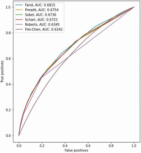
In addition, the ROC curves of the different methods are presented in Figure 16. It shows that Farid achieves the best AUC results, whereas Frei-Chen achieves the worst performance, while Prewitt, Roberts, Scharr and Sobel obtain comparable results. As a result, ROC curve evaluations further support the quantitative evaluations that the Farid operator achieving the best F1, and PPV metrics emerges as the best first-order derivatives-based edge detection method on the dataset.

Figure 16. ROC curves of the first-order derivatives-based edge detectors.

5.2.2. Second-order derivatives

5.2.2.1. Laplacian of Gaussian (LoG)

The quantitative evaluation results for the second-order derivative-based LoG method with different parameters over the training set are provided in Table 3.

Table 3. Evaluation of the different parameters for LoG.

Setup	ACC$\uparrow$	F1$\uparrow$	PPV$\uparrow$	FM$\uparrow$
$\sigma =1.0$	0.6536	0.1894	0.1598	0.2009
$\sigma =1.4$	0.6745	0.1852	0.1632	0.1943
$\sigma =2.0$	0.6988	0.1796	0.1684	0.1866
$\sigma =2.7$	0.7225	0.1734	0.1753	0.1791
$\sigma =3.0$	0.7312	0.1708	0.1783	0.1762

The results show that as the sigma increases, accuracy and PPV tend to increase, whereas F1 and FM scores tend to decrease. It suggests that with extra smoothing false positives are handled better as the accuracy increases. However, it also smears out the true edges thereby lowering the F1 score. Considering our ranking of the metrics, LoG with $\sigma =1$ having the best F1 and FM scores emerges as the best setup. Since we use the inherit the zero-crossing property of the second-order derivatives-based methods for the detection step, ROC curves and the related AUC scores are not realized.

In addition, compared against the first-order derivatives-based methods of Table 2, the performance of the LoG operator is quite poor. For instance, Farid with the highest F1 score achieves 0.3581 and Frei-Chen with the lowest F1 score achieves 0.3053, whereas LoG with the highest F1 can only reach to 0.1894, which is significantly lower. The same pattern is also observed for PPV and FM metrics. This is in compliance with the findings of Bachofer et al. (2016) that LoG is not performing well on SAR images because of the low gradients that are due to the remaining noise negatively influencing the Gaussian filter. As a result, none of the evaluated LoG settings properly suits for SAR images. Nonetheless, we conclude that $\sigma =1$ is the best option for LoG that is to be evaluated on the test data.

5.2.2.2. Difference of Gaussians (DoG)

The quantitative evaluation results for the second-order derivatives-based DoG method with different parameters over the training set are provided in Table 4.

Table 4. Evaluation of the different parameters for DoG. Ratio indicates the size ratio of the kernels.

Setup	ACC$\uparrow$	F1$\uparrow$	PPV$\uparrow$	FM$\uparrow$
${\sigma }_1=1.0$ $|$ ratio = 4	0.7152	0.1757	0.1737	0.1818
${\sigma }_1=1.0$ $|$ ratio = 5	0.7273	0.1725	0.1783	0.1783
${\sigma }_1=1.4$ $|$ ratio = 4	0.7388	0.1690	0.1830	0.1746
${\sigma }_1=1.4$ $|$ ratio = 5	0.7495	0.1655	0.1888	0.1714
${\sigma }_1=2.0$ $|$ ratio = 4	0.7631	0.1596	0.1961	0.1663
${\sigma }_1=2.0$ $|$ ratio = 5	0.7716	0.1555	0.2027	0.1634
${\sigma }_1=2.7$ $|$ ratio = 4	0.7815	0.1486	0.2089	0.1580
${\sigma }_1=2.7$ $|$ ratio = 5	0.7882	0.1441	0.2159	0.1552
${\sigma }_1=3.0$ $|$ ratio = 4	0.7874	0.1440	0.2136	0.1547
${\sigma }_1=3.0$ $|$ ratio = 5	0.7935	0.1394	0.2208	0.1519

The results show that DoG behaves similarly to LoG; as the sigma increases, accuracy and PPV tend to increase, while F1 and FM scores tend to decrease. Likewise, it shows that with extra smoothing false-positives decrease as the accuracy increases, yet it also results in the loss of some of the true edges. The same behaviour is also observed for the effect of the ratios that the higher ratios achieve higher accuracy and PPV, but lower F1 and MK scores. Therefore, DoG with ${\sigma }_1=1.0$ and ${\sigma }_2=4.0$ achieving the highest F1 and FM scores is to be evaluated on the test data.

Moreover, compared with the results of Table 3, DoG achieves better accuracy (0.7935 vs. 0.7312) and PPV (0.2208 vs. 0.1783) scores than LoG, yet LoG obtains better F1 (0.1894 vs. 0.1757) and FM (0.2009 vs. 0.1818) scores. In addition, compared against the first-order derivatives-based methods of Table 2, the performance of the DoG operator is quite poor, similar to the case of LoG. The results further suggests that the first-order derivatives are more robust to noise than the second-order derivatives as further differentiation amplifies the noise. Overall, the evaluations indicate low trustworthiness of the second-order derivatives-based operators for the task.

5.2.3. Advanced methods

5.2.3.1. Canny

The quantitative evaluation results for the advanced Canny method with different parameters over the training set are provided in Table 5.

Table 5. Evaluation of Canny edge detection for different sigma options and threshold ratios.

Setup	ACC$\uparrow$	F1$\uparrow$	PPV$\uparrow$	FM$\uparrow$
$\sigma =1.0$ $|$ ratio = 2	0.7885	0.1829	0.2512	0.1930
$\sigma =1.0$ $|$ ratio = 3	0.7827	0.1826	0.2409	0.1914
$\sigma =1.4$ $|$ ratio = 2	0.7972	0.1793	0.2618	0.1913
$\sigma =1.4$ $|$ ratio = 3	0.7920	0.1791	0.2513	0.1896
$\sigma =2.0$ $|$ ratio = 2	0.8047	0.1736	0.2734	0.1882
$\sigma =2.0$ $|$ ratio = 3	0.8008	0.1735	0.2637	0.1866
$\sigma =2.7$ $|$ ratio = 2	0.8105	0.1664	0.2833	0.1839
$\sigma =2.7$ $|$ ratio = 3	0.8079	0.1665	0.2751	0.1826
$\sigma =3.0$ $|$ ratio = 2	0.7963	0.1632	0.2438	0.1749
$\sigma =3.0$ $|$ ratio = 3	0.8103	0.1632	0.2792	0.1806

The results show that for all the sigma options, the upper:lower threshold ratio of 2:1 achieves better results on all metrics, with an exception for the $\sigma =3$ setup. It suggests that the ratio of 3:1 is more prone to wrongly classifying the weak edges as true edges. Similar to the case of second-order derivatives-based methods presented in Table 3 and Table 4, accuracy and PPV tend to increase as the smoothing factor increases, while F1 and FM scores deteriorate until $\sigma =2.7$, where the metrics start to fluctuate. Therefore, Canny with $\sigma =1.0$ and the ratios of 2:1 achieving the highest F1 and FM scores is to be evaluated on the test data. Finally, non-maximum suppression, double thresholding and hysteresis steps prevent Canny from realizing proper ROC curves. Nonetheless, the AUC results are in parallel with the quantitative results.

In addition, compared against the first-order derivatives-based methods of Table 2, Canny achieves higher accuracy which can be attributed to the additional smoothing step. Nonetheless, it falls behind on other scores. The reason Canny performs poorly is due to the fact that Canny generates one pixel wide edge maps, whereas our dataset includes edges wider than one pixel, which hinders the quantitative performance of Canny on this particular dataset. On the other hand, compared against the best parameter settings of the second-order derivatives-based methods of Table 3 and Table 4, Canny achieves significantly better accuracy and PPV scores, while being on par with F1 and FM scores. Therefore, Canny appears as a better option than the second-order derivatives-based methods for the task. As a final note, replacing its Gaussian filter with a bilateral filter might further improve the results (Fawwaz et al. 2018).

5.2.3.2. Gabor filters

The quantitative evaluation results for the different Gabor filter-banks with various scales and orientations over the training set are provided in Table 6.

Table 6. Evaluation of Gabor edge detection for different scales (S) and orientations (O).

Setup	ACC$\uparrow$	F1$\uparrow$	PPV$\uparrow$	FM$\uparrow$
$S=2$ $|$ $O=3$	0.6208	0.3092	0.2328	0.3478
$S=3$ $|$ $O=5$	0.6113	0.3210	0.2381	0.3650
$S=4$ $|$ $O=6$	0.6147	0.3294	0.2443	0.3749
$S=5$ $|$ $O=8$	0.6440	0.3404	0.2584	0.3819

It shows that for all the metrics, the results tend to improve as the number of scales and orientations increases, because the filter-banks are able to capture more diverse patterns. Further improvements might be attainable by increasing the scale and orientation coverage. Nonetheless, the runtime also grows significantly with the additional variations. For instance, it takes around 500 hours to evaluate $GS5O8$ over the dataset .¹⁰ Thus, we do not gauge additional combinations. In addition, the ROC curves for the different filter banks are presented in Figure 17.

Figure 17. ROC curves of the Gabor filter-banks.

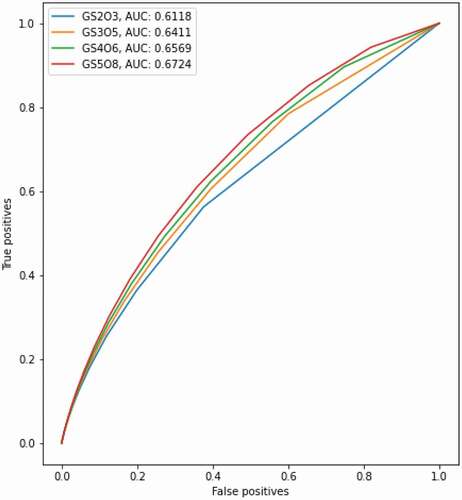
It supports the metrics that increasing the number of scales and orientations further improves the AUC metric. Thus, the Gabor filter-bank with five scales and eight orientations ($GS5O8$) emerges as the best setup which is to be evaluated on the test data.

In addition, compared against the first-order derivatives-based edge detection methods in Table 2, $GS5O8$ is superior to Frei-Chen on all metrics, and it achieves the second best FM scores after Prewitt. Moreover, in terms of AUC, $GS5O8$ obtains better results than Frei-Chen, Roberts and Scharr, yet its performance is not as good as Sobel, Prewitt or Farid. Similarly, compared with Table 4 and Table 3, $GS5O8$ manages to achieve better results than second-order derivatives-based methods on all metrics except for accuracy. Finally, compared against the best performing Canny of Table 5, $GS5O8$ achieves higher F1, FM, and PPV, while obtaining lower accuracy scores. Thus, for applications where attaining high FM levels is more important, the method might be a suitable option. Additionally, as stated by Xiang et al. (2017a) Gabor filters tend to provide better connectivity and smoothness for the SAR image edge detection task, which might be another aspect to consider. Nonetheless, the authors also acknowledge that the computational cost should also be carefully considered, especially given the performance of the Gabor filters is lower or similar compared against the first-order derivatives-based methods. Utilizing log-Gabor wavelets or fuzzified Gabor filter-banks might further improve the results (Nava et al. 2011; Tadic et al. 2021).

5.2.3.3. K-means clustering

The quantitative evaluation results for the K-means clustering-based edge detection method with different number of clusters over the training set are provided in Table 7.

Table 7. Evaluation of different number of clusters for K-means-based edge detection.

Setup	ACC$\uparrow$	F1$\uparrow$	PPV$\uparrow$	FM$\uparrow$
$k=3$	0.7636	0.2747	0.2892	0.2835
$k=4$	0.7200	0.2966	0.2609	0.3108
$k=5$	0.6809	0.3094	0.2467	0.3329

The results resemble the opposite of the second-order derivatives-based evaluations presented in Table 3 and Table 4 in such a way that an increase in the number of clusters also improves F1 and FM scores, while accuracy and PPV scores tend to decrease. For the second-order derivatives-based methods, as the sigma (i.e. smoothing factor) increases, accuracy and PPV also increase since it helps removing a proportion of the remaining noise that is classified as false edges, yet F1 score deteriorates as the extra smoothing also causes some of the true edges to be smeared out. On the other hand, for the K-means clustering-based edge detection, as the number of clusters increases, accuracy and PPV scores drop, and F1 and FM scores increase. The reason behind this is that higher number of clusters also provide higher granularity. As a result, the number of clusters and the smoothing factor are negatively correlated.

In addition, Figure 18 presents the ROC curves for the different k values. It further supports the metrics that $k=5$ achieves the best AUC, whereas $k=3$ appears to be the worst. Nonetheless, the linear behaviour of the ROC curves suggests that this might not be a suitable approach for highly speckled SAR images. To conclude, $k=5$ with the best F1, FM and AUC scores is to be evaluated on the test data.

Figure 18. ROC curves of the K-means clustering-based edge detection.

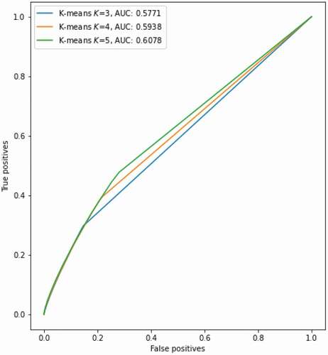
Compared against the first-order derivatives-based edge detection methods of Table 2, $k=5$ obtains better results than Frei-Chen on all metrics, except for FM and AUC scores, and its performance is not as good as any other method over all the metrics. Moreover, compared against the best-performing parameter settings of LoG in Table 3 and DoG in Table 4, $k=5$ outperforms both, except for the accuracy in the case of DoG, which suggests that K-means clustering-based edge detector is a better option than the second-order derivatives-based edge detection methods for the task.

Moreover, compared with Table 5, its performance is significantly better than Canny in terms of F1 (0.3094 vs. 0.1829) and FM (0.3329 vs. 0.1930) scores, whereas Canny’s accuracy is significantly superior (0.6809 vs. 0.7885) which once again shows the contribution of the smoothing process. Finally, comparing $k=5$ against the best-performing Gabor filter-bank of Table 6, $GS5O8$ obtains better F1 (0.3094 vs. 0.3404), PPV (0.2467 vs. 0.2584), FM (0.3329 vs. 0.3819) and AUC (0.6078 vs. 0.6724) scores, while being worse only on accuracy (0.6809 vs. 0.6440). To conclude, although $k=5$ is capable of outperforming the second-order derivatives-based methods, its performance is not as promising as the first-order derivatives-based methods and also Gabor filters. The reason might be that the K-means clustering unnecessarily oversimplifies the scene reflectivity causing some of the true edges to fade out. Constraining the clustering process by spatial consistency or incorporating additional features (e.g. texture) might further improve the results (Gou et al. 2018; Shang et al. 2020).

5.2.3.4. 2D discrete wavelet transformation

The quantitative evaluation results for the 2D discrete wavelet transformation-based edge detection are provided in Table 8. Additionally, the AUC metric with the accompanying ROC curve is presented in Figure 19. Note that similar to the case of first-order derivatives-based methods, we do not evaluate for different hyperparameters.

Figure 19. ROC curve of the 2D Discrete Wavelet Transformation-based edge detection.

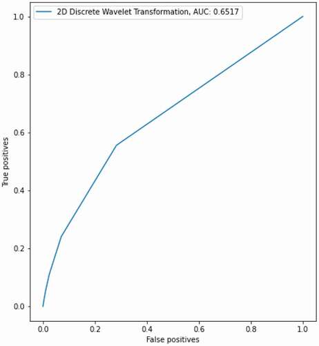
Table 8. Evaluation of 2D discrete wavelet transformation-based edge detection.

Setup	ACC$\uparrow$	F1$\uparrow$	PPV$\uparrow$	FM$\uparrow$
2D Discrete Wavelet	0.7000	0.3557	0.2855	0.3852

Firstly, compared with the first-order derivatives-based edge detection methods in Table 2, it achieves similar F1 scores, it is better than Frei-Chen on all metrics, and it has the best FM score which indicates that the method is capable of achieving better recall rates. In terms of AUC, it again achieves better results than Frei-Chen and also Roberts, yet it is worse than the rest. Secondly, compared against the second-order derivatives-based edge detection methods in Table 3 and in Table 4 and the advanced Canny in Table 5, it achieves better results on all metrics, except for accuracy, which is due to the smoothing features of LoG and DoG. Similarly, compared with Table 7, it is superior to K-means clustering-based edge detector on all metrics. On the other hand, its performance is not as superior as Gabor filter-banks presented in Table 6 so that it can only obtain better results on accuracy, while being on par with the FM scores. As a conclusion, 2D discrete wavelet transformation-based edge detection emerges as a promising alternative for the task. Additional levels of decomposition might further improve the results (Maksimovic et al. 2019).

5.2.3.5. Subpixel edge detector

The quantitative evaluation results for the advanced subpixel edge detection method for different iterations over the training set are provided in Table 9.

Table 9. Evaluation of different iterations for the subpixel-based edge detection method.

Setup	ACC$\uparrow$	F1$\uparrow$	PPV$\uparrow$	FM$\uparrow$
$iter=1$	0.7330	0.1581	0.1701	0.1634
$iter=2$	0.7005	0.1754	0.1650	0.1820
$iter=3$	0.6963	0.1772	0.1643	0.1840

The results show that the best accuracy and PPV is achieved with a single iteration, whereas the best F1 and FM is achieved with three iterations. The accuracy and PPV tend to deteriorate with additional iterations, while F1 and FM tend to improve. It means that the method achieves better recall with extra restoration steps. The performance appears to converge with three iterations, which is in line with the findings of the authors that a few iterations are sufficient Trujillo-Pino et al. (2013). As a result, the subpixel edge detection method with three iterations is to be evaluated on the test data.

Additionally, compared with the first-order derivatives-based edge detection methods in Table 2, it only achieves better results than Frei-Chen in terms of accuracy, whereas its performance is worse than others on all metrics. Moreover, its performance is very similar to the second-order derivatives-based edge detection methods provided in Table 3 and in Table 4. Furthermore, compared against the methods that are considered advanced, it can only achieve better accuracy levels than Gabor and K-means clustering-based edge detector, while its performance is worse than others on all metrics. It suggests that this method is not convenient for the task given its relatively low performance with its complex nature. Utilizing a moments-based subpixel edge localization method might achieve improved results (Renshaw and Christian, 2020). Finally, it is worth mentioning that the method generates thin edges, which as stated before does not well suited for our benchmark. Furthermore, the method generates very low-valued edge responses, meaning that the most of the edge responses do not pass our second lowest threshold of 0.05. Using a more fine-grained thresholding scheme might further improve the results.

5.2.4. SAR-specific methods

5.2.4.1. Touzi

The quantitative evaluation results for the SAR-specific Touzi method with different radius values over the training set are provided in Table 10. In addition, the ROC curve of Touzi for different parameters are presented in Figure 20.

Figure 20. ROC curves of Touzi for different radius values.

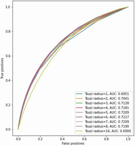
Table 10. Evaluation of different parameters for Touzi.

Setup	ACC$\uparrow$	F1$\uparrow$	PPV$\uparrow$	FM$\uparrow$
$radius=1$	0.7582	0.3739	0.3366	0.3922
$radius=2$	0.7267	0.3788	0.3159	0.4051
$radius=3$	0.7515	0.3866	0.3351	0.4071
$radius=4$	0.7304	0.3899	0.3186	0.4162
$radius=5$	0.7132	0.3892	0.3067	0.4204
$radius=6$	0.7438	0.3877	0.3254	0.4099
$radius=7$	0.7319	0.3852	0.3150	0.4103
$radius=8$	0.7208	0.3817	0.3057	0.4094
$radius=16$	0.6492	0.3510	0.2562	0.3932

The results show that the best accuracy and precision are achieved with radius of 1. The best F1-score is achieved with radius of 4, and the radius of 16 results deviates from the rest. Moreover, the best Fowlkes–Mallows index is achieved with radius of 5. Since there is no clear difference between different setups and F1 scores differ in the fourth significant figure, we use the guidance of the AUC metric to decide the best-performing one. It can be observed that the method achieves the best AUC metric (0.7217) using radius of 6. The metric tends to increase until 6, then starts decreasing. Although Touzi using radius of 4 achieves the best F1 score, we deem Touzi with radius of 6 as the best option which is to be evaluated on the test data, as the differences in F1 is very marginal and it achieves better AUC, PPV and accuracy than using 4.

In addition, compared against the first-order derivatives-based edge detection methods of Table 2, Touzi with radius of 6 obtains better F1, FM, and AUC scores which shows the superiority of the SAR specific Touzi over the traditional optical edge detection methods. Nonetheless, its performance is not as good as some on accuracy and PPV, which suggests that Touzi has better recall rate overall. Furthermore, compared against the best-performing parameter settings of LoG in Table 3 and DoG in Table 4, Touzi outperforms both achieving scores 2 times better, except for accuracy where they obtain similar results. The same behaviour is also observed comparing against Canny in Table 5. Similarly, it has better performance than Gabor filter-banks of Table 6, K-means clustering-based edge detection method of Table 7 and 2D discrete wavelet transformation-based edge detection of Table 8 and the subpixel-based method of Table 9 on all metrics. Finally, the behaviour of the ROC curve further supports that this SAR-specific method is overall a better option than the previously evaluated methods.

5.2.4.2. Gradient by ratio (GR)

The quantitative evaluation results for the SAR-specific GR method with different smoothing factors ($\alpha$) over the training set are provided in Table 11.

Table 11. Evaluation of different parameters for GR.

Setup	ACC$\uparrow$	F1$\uparrow$	PPV$\uparrow$	FM$\uparrow$
$\alpha =1$	0.6956	0.3365	0.3007	0.3736
$\alpha =2$	0.7319	0.3610	0.3198	0.3885
$\alpha =3$	0.7088	0.3705	0.3039	0.4032
$\alpha =4$	0.6867	0.3708	0.2893	0.4087
$\alpha =5$	0.6704	0.3677	0.2790	0.4092
$\alpha =6$	0.6551	0.3633	0.2699	0.4081

The results show that the best accuracy is obtained by $\alpha =3$, and the best precision by $\alpha =4$. Moreover, F1 and FM scores improve as the smoothing factor increases until $\alpha =5$, then they starts deteriorating. In addition, the ROC curve of GR for different parameters are presented in Figure 21. Similarly, the results tend to improve with higher smoothing factors, yet they converge around $\alpha =4$ achieving the best AUC metric (0.7037). As a conclusion, GR with $\alpha =4$ achieving the best F1 and AUC scores is to be used to evaluate the test data.

Figure 21. ROC curves of GR for different sigma values.

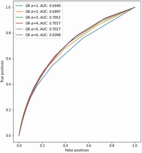
In addition, compared against the first-order derivatives-based methods of Table 2, GR with $\alpha =4$ obtains better F1, FM and AUC scores, yet its performance is not as good as others on accuracy and PPV, similar to the case of Touzi. Thus, the method has a better recall rate than the first-order derivatives-based methods. It is also better than Frei-Chen on all metrics. Furthermore, compared against the best-performing parameter settings of LoG in Table 3 and DoG in Table 4, and also with the advanced Canny in Table 5 and the advanced subpixel-based edge detector in Table 9, GR with $\alpha =4$ is superior on all metrics, except for the accuracy. Moreover, it has better performance than Gabor filter-banks presented in Table 6, K-means clustering-based edge detection method in Table 7 and 2D discrete wavelet transformation-based edge detection in Table 8. However, the best-performing Touzi presented in Table 10 appears better than the best-performing GR on all metrics. Therefore, Touzi using the ratio of the averages (ROA) achieves superior results than GR using the ratio of exponentially weighted averages (ROEWA) over this dataset. Nonetheless, both methods obtain preferable performance over the non-SAR-specific methods.

5.2.4.3. Gaussian-Gamma-shaped (GSS) bi-windows

The quantitative evaluation results for the SAR-specific Gaussian-Gamma-shaped bi-windows method with different parameters for $alpha$ controlling the window with for different width and length values over the training set are provided in Table 12.

Table 12. Evaluation of different parameters for the Gaussian-Gamma-shaped bi-windows.

Setup	ACC$\uparrow$	F1$\uparrow$	PPV$\uparrow$	FM$\uparrow$
$\alpha =2|w=7.0|l=6.5$	0.8109	0.1453	0.2675	0.1642
$\alpha =2|w=7.0|l=7.0$	0.8111	0.1458	0.2689	0.1648
$\alpha =2|w=9.0|l=6.5$	0.8150	0.1372	0.2746	0.1590
$\alpha =2|w=9.0|l=7.0$	0.8149	0.1378	0.2749	0.1594
$\alpha =3|w=7.0|l=6.5$	0.8084	0.1420	0.2544	0.1593
$\alpha =3|w=7.0|l=7.0$	0.8086	0.1426	0.2554	0.1599
$\alpha =3|w=9.0|l=6.5$	0.8147	0.1324	0.2666	0.1537
$\alpha =3|w=9.0|l=7.0$	0.8144	0.1328	0.2661	0.1539
$\alpha =4|w=7.0|l=6.5$	0.8199	0.1384	0.3028	0.1649
$\alpha =4|w=7.0|l=7.0$	0.8197	0.1387	0.3026	0.1651
$\alpha =4|w=9.0|l=6.5$	0.8156	0.1273	0.2643	0.1492
$\alpha =4|w=9.0|l=7.0$	0.8154	0.1276	0.2638	0.1493

The results show that the best accuracy and precision are achieved with alpha of 4, width 7 and length 6.5. The best F1-score is achieved with alpha of 2, width 7 and length 7. Moreover, the best Fowlkes–Mallows index is achieved with alpha of 4, width 7 and length 7. As the width increases, F1 and FM scores tend to decrease. Moreover, as the length increases, F1 scores tend to increase. On the other hand, there is no significant difference between different setups. Therefore, GSS bi-windows with $\alpha =2,w=7,l=7$ achieving the best F1-score is to be utilized on the test data. In addition, compared against the first-order derivatives-based edge detection methods of Table 2, GSS bi-windows with $\alpha =2,w=7,l=7$ obtains better accuracy scores, yet its performance is not as good as others on F1 and FM scores, and comparable PPV scores. Furthermore, compared against the best-performing parameter settings of LoG in Table 3 and DoG in Table 4, and also with the advanced Canny in Table 5 and the advanced subpixel-based edge detector in Table 9, GSS achieves better accuracy and PPV, and comparable results on F1 and FM scores. Moreover, it has better accuracy and PPV performance than Gabor filter-banks presented in Table 6, K-means clustering-based edge detection method in Table 7 and 2D discrete wavelet transformation-based edge detection in Table 8, yet it has significantly worst performance on F1 and FM scores. Additionally, the best-performing Touzi model presented in Table 10 and the best-performing GR model presented in Table 11 appears superior than the best-performing GSS bi-windows on all metrics, except for accuracy. Therefore, Touzi and GR using rectangular bi-windows achieves superior results than using Gaussian-Gamma-shaped bi-windows over this dataset.

5.2.4.4. ROLSS RUSTICO

The quantitative evaluation results for the SAR-specific ROLSS RUSTICO method with different noise suppression levels over the training set are provided in Table 13.

Table 13. Evaluation of different parameters for ROLSS RUSTICO.

Setup	ACC$\uparrow$	F1$\uparrow$	PPV$\uparrow$	FM$\uparrow$
$\xi =1.0|\lambda =0.5$	0.7718	0.1475	0.2352	0.1644
$\xi =1.0|\lambda =1.0$	0.7700	0.1489	0.2355	0.1658
$\xi =1.0|\lambda =2.0$	0.7681	0.1529	0.2366	0.1696
$\xi =1.0|\lambda =3.0$	0.7607	0.1607	0.2324	0.1763
$\xi =1.5|\lambda =0.5$	0.7727	0.1479	0.2359	0.1647
$\xi =1.5|\lambda =1.0$	0.7700	0.1496	0.2361	0.1665
$\xi =1.5|\lambda =2.0$	0.7676	0.1544	0.2370	0.1710
$\xi =1.5|\lambda =3.0$	0.7590	0.1634	0.2319	0.1787
$\xi =2.0|\lambda =0.5$	0.7736	0.1482	0.2365	0.1650
$\xi =2.0|\lambda =1.0$	0.7701	0.1501	0.2365	0.1671
$\xi =2.0|\lambda =2.0$	0.7672	0.1554	0.2373	0.1720
$\xi =2.0|\lambda =3.0$	0.7578	0.1649	0.2315	0.1801

The results show that the best accuracy is realized with ($\xi =2.0,\lambda =0.5$), the best PPV is with ($\xi =2.0,\lambda =2.0$), and the best F1 and FM scores with ($\xi =2.0,\lambda =3.0$). In addition, as the size of the image region in which the noise is suppressed ($\lambda$) increases the results tend to improve. Moreover, as the strength of the suppression ($\xi$) increases, accuracy tend to decrease, whereas F1 and FM scores increase with extra suppression. As a conclusion, ($\xi =2,\lambda =3$) achieving the best F1 and FM scores is to be evaluated on the test data.

Furthermore, compared against the first-order derivatives-based edge detection methods of Table 2, ROLSS RUSTICO achieves comparable accuracy levels, but its performance is not as good on other metrics. Moreover, compared against the best-performing parameter settings of LoG in Table 3 and DoG in Table 4, ROLSS RUSTICO has better accuracy and PPV scores. In addition, compared against the advanced Gabor filters in Table 6, K-means clustering-based edge detection method in Table 7, 2D discrete wavelet transformation-based edge detection in Table 8, and subpixel-based edge detector in Table 9 ROLSS RUSTICO attain higher accuracy scores. On the other hand, the results presented for Canny in Table 5 appear superior on all metrics. Additionally, compared against the SAR-specific Touzi presented in Table 10 and GR presented in Table 11, ROLSS RUSTICO again obtains higher accuracy scores, but its performance is worse on all other metrics. Finally, ROLSS RUSTICO is capable of achieving better F1 and FM scores than GSS bi-windows presented in Table 12, yet its accuracy and PPV is lower. All in all, the performance of ROLSS RUSTICO suggest that the method might be considered for applications aiming high accuracy.

5.2.4.5. SAR-Shearlet

The quantitative evaluation results for the SAR-specific SAR-Shearlet method with parameters over the training set are provided in Table 14.

Table 14. Evaluation of different parameters for SAR-Shearlet, where $l$ denotes the effective support length of the Mexican hat wavelet.

Setup	ACC$\uparrow$	F1$\uparrow$	PPV$\uparrow$	FM$\uparrow$
$Shearlevel=2|scales=2|l=1/2$	0.7660	0.2836	0.2960	0.2963
$Shearlevel=2|scales=3|l=1/2$	0.1595	0.2680	0.1595	0.3876
$Shearlevel=2|scales=2|l=1/7$	0.1595	0.2680	0.1595	0.3876
$Shearlevel=2|scales=3|l=1/7$	0.1595	0.2680	0.1595	0.3876
$Shearlevel=3|scales=2|l=1/7$	0.1595	0.2680	0.1595	0.3876
$Shearlevel=3|scales=3|l=1/7$	0.1595	0.2680	0.1595	0.3876
$Shearlevel=4|scales=2|l=1/7$	0.1595	0.2680	0.1595	0.3876
$Shearlevel=4|scales=3|l=1/7$	0.1595	0.2680	0.1595	0.3876

The results show that increasing the shear levels does not have an effect over the results. Moreover, increasing the number of scales might negatively effect the performance as can be observed from shear levels of 2. Shear levels with $l=1/7$ result in very poor performance. The accuracy scores are so low that one might achieve the same results by classifying each pixel as an edge. On the other hand, increasing the effective support length of the Mexican hat wavelet to $1/2$ significantly improves accuracy and PPV scores, while deteriorating FM scores. Similarly, a clear improvement in ROC AUC can be observed increasing the effective support length of the Mexican hat wavelet, as presented in Figure 22. To conclude, SAR-Shearlet with ($Shearlevel=2,scales=2,l=1/2$) is to be evaluated on the test set.

Figure 22. ROC curves of SAR-Shearlet for different parameters.

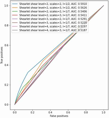
Furthermore, compared against the first-order derivatives-based edge detection methods of Table 2, SAR-Shearlet achieves better accuracy and comparable PPV levels, but its performance is not as good on F1 and FM scores. In addition, compared against the second-order derivatives based of LoG in Table 3 and DoG in Table 4, and also against the advanced subpixel-based edge detector in Table 9, SAR-Shearlet obtains superior performance on all metrics. Moreover, it achieves better accuracy and PPV scores compared against the advanced Gabor filters in Table 6, K-means clustering-based edge detection method in Table 7 and 2D discrete wavelet transformation-based edge detection in Table 8. On the other hand, its performance is better than Canny, presented in Table 5, only in terms of accuracy. Finally, compared against the SAR-specific Touzi presented in Table 10, it has better accuracy; against GR presented in Table 11, it has better accuracy and PPV; against GSS bi-windows presented in Table 12, it has better F1, PPV and FM; and against ROLSS RUSTICO presented in Table 13, it obtains superior results on all metrics.

5.2.5. Fusion

5.2.5.1. Binary decision fusion

In this section, we evaluate two fundamental binary decision fusion methods; ($a$) single voting where at least one of the methods has to classify a pixel an edge (logical disjunction) and ($b$) complete agreement where all the methods should classify a pixel an edge (logical conjunction), to combine the final outputs of multiple methods into a final ensemble decision. In this setup, each detector has the same voting power. The thresholding for each method is realized by choosing the threshold that produce the highest average F1-score over the complete training set. To that end, we combine ($i$) SAR-specific Touzi and the best-performing optical method, Farid, and ($ii$) SAR-specific ROA-based Touzi and SAR-specific ROEWA-based GR to exploit their different features. The quantitative evaluation results for the different voting combinations and methods are presented in Table 15 and Table 16.

Table 15. Evaluation of the fusion schemes for combining the SAR-specific Touzi and optical Farid methods.

Setup	ACC$\uparrow$	F1$\uparrow$	PPV$\uparrow$	FM$\uparrow$
Single voting	0.6816	0.3739	0.2816	0.4117
Complete agreement	0.8104	0.3735	0.4143	0.3847
Touzi($r=6$)	0.7438	0.3877	0.3254	0.4099
Farid	0.7483	0.3581	0.3300	0.3768

Table 16. Evaluation of the fusing schemes for combining the ROA-based Touzi and ROEWA-based GR.

Setup	ACC$\uparrow$	F1$\uparrow$	PPV$\uparrow$	FM$\uparrow$
Single voting	0.6803	0.3793	0.2891	0.4186
Complete agreement	0.7502	0.3792	0.3259	0.4001
Touzi($r=6$)	0.7438	0.3877	0.3254	0.4099
GR($\alpha =4$)	0.6867	0.3708	0.2893	0.4087

The results show that exploiting the best of the two worlds (SAR-specific and optical) provides significantly better accuracy (0.7438 $\to$ 0.8104) and PPV (0.3254 $\to$ 0.4143) scores using the complete agreement scheme. It achieves better results than fusing two SAR-specific methods. To that end, we select the complete agreement scheme fusing Touzi and Farid as the best-performing binary decision fusion method. Moreover, as it is a pixel-wise binary operation, it does not significantly affect the computational complexity. Therefore, application aiming higher accuracy and PPV scores should consider this fusion scheme. Incorporating additional methods to the fusion process or exploring other fusion schemes (e.g. majority voting) might provide additional improvements.

5.2.5.2. Gradient magnitude fusion

In this section, instead of combining the binary outputs, we combine the real-valued gradient magnitudes. To that end, we compute the averages of ($i$) Farid and Touzi, and ($ii$) Touzi and GR, similar to the binary decision fusion experiments. The quantitative evaluation results for the gradient magnitude fusion and the related methods are presented in Table 17 and Table 18.

Table 17. Evaluation of the gradient magnitude fusion for the SAR-specific Touzi and non-SAR Farid method.

Setup	ACC$\uparrow$	F1$\uparrow$	PPV$\uparrow$	FM$\uparrow$
Gradient Fusion	0.7481	0.3933	0.3313	0.4149
Touzi($r=6$)	0.7438	0.3877	0.3254	0.4099
Farid	0.7483	0.3581	0.3300	0.3768

Table 18. Evaluation of the gradient magnitude fusion for combining the ROA-based Touzi and ROEWA-based GR.

Setup	ACC$\uparrow$	F1$\uparrow$	PPV$\uparrow$	FM$\uparrow$
Gradient Fusion	0.7237	0.3854	0.3108	0.4133
Touzi($r=6$)	0.7438	0.3877	0.3254	0.4099
GR($\alpha =4$)	0.6867	0.3708	0.2893	0.4087

The results show that the gradient fusion of Farid and Touzi provides better F1 (0.3877 $\to$ 0.3933), PPV (0.3254 $\to$ 0.3313), and FM (0.4099 $\to$ 0.4149) scores, whereas the combination of Touzi and GR only achieves better FM score. Therefore, similar to the case of the binary fusion experiments, exploiting the best of the two worlds provides better results, which is also confirmed by the ROC curves presented in Figure 23. To that end, we conclude that gradient fusion of Touzi and Farid has the superior performance which is to be utilized for the test set. Incorporating a weighting scheme to adjust the contributions of the algorithms might further improve the results.

Figure 23. ROC curve of gradient fusion.

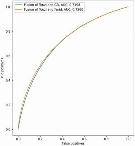
5.2.6. Overview of the best performing parameters

To conclude the experiments on the training set, Table 19 provides a comparison with the best performing parameters that are to be evaluated on the benchmark.

Table 19. Overview of the best performing methods over the training set, ranked by F1-score.

Algorithm	ACC$\uparrow$	F1$\uparrow$	PPV$\uparrow$	FM$\uparrow$
GGS bi-windows ($\alpha =2|w=7|l=7$)	0.8111	0.1458	0.2689	0.1648
ROLSS RUSTICO ($\xi =2|\lambda =3$)	0.7578	0.1649	0.2315	0.1801
DoG(${\sigma }_1=1.0$ $|$ ratio = 4)	0.7152	0.1757	0.1737	0.1818
Subpixel ($iter=3$)	0.6963	0.1772	0.1643	0.1840
Canny ($\sigma =1.0$ $|$ ratio = 2)	0.7885	0.1829	0.2512	0.1930
LoG ($\sigma =1.0$)	0.6536	0.1894	0.1598	0.2009
Shearlet $(Shearlevel=2|scales=2|l=1/2)$	0.7660	0.2836	0.2960	0.2963
Frei-Chen	0.5540	0.3053	0.2102	0.3584
K-means ($k=5$)	0.6809	0.3094	0.2467	0.3329
Gabor (GS5O8)	0.6440	0.3404	0.2584	0.3819
Roberts	0.7530	0.3498	0.3192	0.3665
2D Discrete Wavelet	0.7000	0.3557	0.2855	0.3852
Scharr	0.7606	0.3563	0.3296	0.3715
Sobel	0.7259	0.3573	0.3024	0.3795
Prewitt	0.7168	0.3576	0.2972	0.3823
Farid	0.7483	0.3581	0.3300	0.3768
GR ($\alpha =4$)	0.6867	0.3708	0.2893	0.4087
Binary Fusion	0.8104	0.3735	0.4143	0.3847
Touzi ($r=6$)	0.7438	0.3877	0.3254	0.4099
Gradient Fusion	0.7481	0.3933	0.3313	0.4149

It reveals that the best accuracy is achieved by SAR-specific GSS bi-windows by a large margin. The only exception is the binary fusion of SAR-specific Touzi and traditional first-order derivatives-based Farid which not only achieves the best PPV score, but also obtains comparable accuracy levels to GSS bi-windows, which shows its superiority on handling the ambiguities in identifying the true positives. Moreover, the gradient fusion achieves the best F1 and FM scores which shows its superior performance on handling ambiguities in identifying false positives. Finally, the best performing individual methods are the SAR-specific methods Touzi and GR, followed by the traditional first-order derivatives-based Farid operator over the training set.

5.3. BSDS500-speckled benchmark

In order to provide a more comprehensive comparison and form our SAR image edge detection benchmark, we use the ground-truths and metrics from the original BSDS500 benchmark. The images are first corrupted with 1-look speckles and then denoised as done in the previous sections. To that end, firstly, the gradient (edge response) maps of every edge detector are computed with the parameters determined over the training set. Then, these edge maps are compared to the ground-truths to form the benchmark. As suggested by the developers of the original BSDS500 dataset, three metrics are used to compare the different algorithms: ODS F1 (fixed contour threshold for 200 images), OIS F1 (best threshold for each image), and average precision (AP). The results are provided using 30 different threshold levels in Table 20. For each method, the threshold corresponding to the best ODS F1 score is also provided.

Table 20. BSDS500-speckled Benchmark. The rows are sorted by ODS F1. The best results are highlighted in bold, while the second best results are underlined.

Algorithm	OIS (F1)	ODS (F1)	AP	Threshold
Subpixel ($iter=3$)	0.3019	0.3013	0.1775	0.1290
LoG ($\sigma =1.0$)	0.3333	0.3329	0.1999	0.7097
DoG (${\sigma }_1=1.0$ $|$ ratio = 4)	0.3902	0.3899	0.2453	0.3871
GS5O8	0.4407	0.3965	0.3660	0.1613
ROLSS RUSTICO ($\xi =2|\lambda =3$)	0.4194	0.4190	0.3563	0.0645
K-means ($k=5$)	0.5349	0.4778	0.3336	0.1936
Canny ($\sigma =1.0$ $|$ ratio = 2)	0.4838	0.4835	0.3467	0.6774
Gradient Fusion	0.4859	0.4856	0.3517	0.0968
Shearlet $(Shearlevel=2|scales=2|l=1/2)$	0.5132	0.5022	0.4293	0.0645
2D Discrete Wavelet	0.5428	0.5303	0.5278	0.0645
Farid	0.5599	0.5303	0.4913	0.1613
GGS bi-windows ($\alpha =2|w=7|l=7$)	0.5332	0.5329	0.3988	0.3226
Roberts	0.5470	0.5334	0.5254	0.0645
Sobel	0.5547	0.5350	0.4983	0.1290
Prewitt	0.5550	0.5353	0.4815	0.1290
Scharr	0.5525	0.5356	0.4467	0.0968
Frei-Chen	0.5481	0.5429	0.4430	0.9032
GR ($\alpha =4$)	0.5807	0.5437	0.5194	0.1613
Binary Fusion	0.5583	0.5581	0.6211	0.8710
Touzi ($r=6$)	0.5922	0.5672	0.5437	0.2903
Gradient Fusion	0.6015	0.5820	0.5493	0.4516
GRHED($\alpha =2,3,4,5$) (Liu et al. 2020)	0.6119	0.6115	0.6450	0.7419

It shows that among the methods we provide, the fusion methods achieve the best results. Gradient fusion achieves the best ODS F1 and OIS F1, while the binary fusion of SAR-specific Touzi and traditional Farid with the complete agreement scheme obtains the best AP results. Moreover, comparing the SAR-specific algorithms, Touzi $>$ GR $>$ GSS bi-windows $>$ Shearlet $>$ ROLSS RUSTICO ranking emerges. In addition, similar to the earlier experiments, subpixel-based edge detector, LoG and DoG obtain the lowest scores, while the first-order derivatives-based methods turn out to be very competitive baselines. Furthermore, advanced methods do not perform well, except for the 2D Discrete Wavelet method which obtains comparable results with the traditional methods. On the other hand, overall best results are achieved by the GRHED model, the supervised CNN architecture of Liu et al. (2020), on all metrics which shows the power of the supervised CNNs. Nonetheless, the performance gap between GRHED and the gradient fusion on OIS F1 and ODS F1, and GRHED and the binary fusion on AP is not major, which suggests that the fusion methods are promising alternatives.

5.4. BSDS500-speckled noisy benchmark

Since SAR images are highly corrupted with speckle noise and it is not possible to entirely denoise the speckled images, the anti-noise ability (robustness to the noise) is also an important factor for SAR-specific edge detectors. Moreover, image denoising can be a time-consuming process, and thus time critical applications might want to get rid of the denoising (smoothing) process and directly use the edge detectors on the noisy (corrupted) data. Therefore, in order to provide an even more comprehensive comparison, we present a second benchmark of noisy images to directly measure the performance of the edge detectors, without including any pre-processing step. To that end, we repeat the process of the previous section excluding the denoising process. As a result, the edge detectors are evaluated using noisy SAR images to assess their noise robustness. The results are provided in Table 21 with the thresholds corresponding to the best ODS F1 score.

Table 21. BSDS500-speckled Noisy Benchmark. The rows are sorted by ODS F1. The best results are highlighted in bold, while the second best results are underlined.

Algorithm	OIS (F1)	ODS (F1)	AP	Threshold
GGS bi-windows ($\alpha =2|w=7|l=7$)	0.3622	0.3618	0.2217	0.4194
ROLSS RUSTICO ($\xi =2|\lambda =3$)	0.4142	0.4137	0.3401	0.3226
Shearlet $(Shearlevel=2|scales=2|l=1/2)$	0.5130	0.4950	0.4000	0.3226
Binary Fusion	0.5403	0.5396	0.4252	0.0323
GR ($\alpha =4$)	0.5893	0.5459	0.4744	0.1935
Gradient Fusion	0.5719	0.5533	0.5049	0.5806
Touzi ($r=6$)	0.5928	0.5703	0.5068	0.3871
GRHED ($\alpha =2,3,4,5$) (Liu et al. 2020)	0.6510	0.6505	0.5863	0.2903

The experiments produce similar outcomes considering the top three performing methods such that GRHED $>$ Touzi $>$ Gradient Fusion of Touzi and Farid ranking emerges. GRHED achieves better results on this benchmark as it is trained on noisy inputs. All the single algorithms obtain similar results as the denoised benchmark evaluations which shows the high robustness of the algorithms to the speckle noise. The exception is the GGS bi-windows whose performance significantly deteriorates on the noisy benchmark; OIS (0.5332 $\to$ 0.3622) −32%, ODS (0.5329 $\to$ 0.3618) −32% and AP (0.3988 $\to$ 0.2217) −44%. It suggest that the noise handling capacity of the algorithm needs further attention. Finally, considering the fusion methods, the binary fusion obtains similar OIS and ODS scores, yet AP drops significantly (−31%) on the noisy benchmark (0.6211 $\to$ 0.4252). The gradient fusion scores also deteriorate; OIS (0.6015 $\to$ 0.5719), ODS (0.5820 $\to$ 0.5533) and AP (0.5493 $\to$ 0.5049), but on average the performance drop is around 5% over all metrics. Thus, the gradient fusion method appears more robust to noise. Nonetheless, the results suggest that the fusion methods perform best with a denoising pre-processing step.

5.5. SAR image evaluations

5.5.1. Sentinel-1 Lelystad

Firstly, we consider a single look Sentinel-1 image (1024 x1536 pixels) of Lelystad, Flevoland, Netherlands by Dalsasso et al. (2021). It is denoised the same way as the BSDS500-speckled images by using SARBLF algorithm. Then, the edge detectors are evaluated on the denoised image with the optimal settings derived from the BSDS500-speckled training set. The edge responses are normalized and thresholded with the thresholds found optimal for the F1 score over the training set, as provided in Table 22. To that end, quantitative evaluation is challenging as human annotated ground truth is not available for this image. Nonetheless, following the setup of Liu et al. (2020), we utilize a pseudo ground-truth generated by Xie and Tu (2015) to provide quantitative evaluations, as presented in Figure 24 and in Table 22.

Figure 24. A) Original clean Sentinel-1 Lelystad image. Credits image: Dalsasso et al. (2021) b) Pseudo ground-truth. Credits image: Liu et al., (2020) c) 1-look speckled image. d) Denoised 1-look image.

Table 22. The performances of different methods on the Sentinel-1 Lelystad, ordered by F1 score.

Algorithm	ACC$\uparrow$	F1$\uparrow$	PPV$\uparrow$	FM$\uparrow$	Threshold
ROLSS RUSTICO ($\xi =2|\lambda =3$)	0.9046	0.0462	0.0504	0.0463	0.05
Subpixel	0.7265	0.1036	0.0630	0.1355	0.0
LoG ($\sigma =1.0$)	0.6987	0.1062	0.0632	0.1445	-
DoG (${\sigma }_1=1.0$ $|$ ratio = 4)	0.7749	0.1143	0.0726	0.1395	-
Shearlet $(Shearlevel=2|scales=2|l=1/2)$	0.7944	0.1710	0.1094	0.2069	0.05
GS5O8	0.9066	0.1760	0.1686	0.1762	0.2
Frei-Chen	0.6904	0.1971	0.1147	0.2836	0.45
GGS bi-windows ($\alpha =2|w=7|l=7$)	0.9142	0.1972	0.1998	0.1972	0.15
K-means ($k=5$)	0.7700	0.2075	0.1275	0.2662	0.05
Canny ($\sigma =1.0$ $|$ ratio = 2)	0.9154	0.2325	0.2287	0.2325	0.15
Wavelet	0.7814	0.2572	0.1576	0.3318	0.05
GR ($\alpha =4$)	0.7972	0.2635	0.1640	0.3314	0.15
GRHED ($\alpha =2,3,4,5$) (Liu et al. 2020)	0.9370	0.2817	0.3681	0.2898	0.5516
Touzi ($r=6$)	0.8625	0.2896	0.2011	0.3226	0.3
Prewitt	0.8602	0.3034	0.2078	0.3417	0.1
Roberts	0.8791	0.3057	0.2219	0.3302	0.05
Farid	0.9184	0.3060	0.2839	0.3069	0.15
Binary Fusion	0.9260	0.3064	0.3111	0.3065	-
Sobel	0.8742	0.3101	0.2207	0.3393	0.1
Gradient Fusion	0.8822	0.3120	0.2282	0.3354	0.45
Scharr	0.8847	0.3150	0.2323	0.3371	0.1

The results show that the best F1 score is achieved by the traditional Scharr operator, while the best accuracy and precision are achieved with the supervised CNN model GRHED, and the best FM score is obtained by the traditional Prewitt. Moreover, the binary fusion of Touzi and Farid using the complete agreement scheme achieves the second best performance on accuracy and precision, whereas the traditional Sobel obtains the second best performance on FM score. In addition, the gradient fusion of Touzi and Farid achieves the second best performance on F1 score. The results are in line with the BSD500-speckled benchmark evaluations such that the first-order derivatives-based methods turn out to be very competitive baselines. On the other hand, SAR-specific ROLSS RUSTICO and Shearlet both have very low performances, which might suggest that the parameters of these algorithms are sensitive to different cases, and therefore leading to poor generalization performance.

In addition, Figure 25 presents the outputs of a number of methods to qualitatively assess their performances by evaluating the detection performances over the homogeneous regions such as the agricultural fields and water bodies, and the linear structures such as the roads and field boundaries.

Figure 25. Edge detection performances on a single look Sentinel-1 image of Lelystad.

The results show that the second-order derivatives-based DoG and the advanced subpixel-based edge detection methods completely fail generating outputs resembling white noise patterns. The Gabor filters (GS5O8) are confused by the large gradients caused by the very bright pixels, thus only the brightest pixels are recognized as edges. These methods appear unfit for the edge detection task on SAR images. In addition, Canny and K-means seem to be to rather sensitive to the speckle noise patterns over the land area, yet they can handle the homogeneous water bodies. 2D discrete wavelet method can capture linear structures of the borders between the agricultural fields, yet the output is highly corrupted with salt-and-pepper like noise patterns and thus does not appear useful for derivative applications. Scharr results are similar to 2D discrete wavelet, but it handles the separation between homogeneous regions better, has less noise, and the linear structures are more differentiable.

As for the SAR-specific methods, Shearlet performs well for capturing the bankline structure between the land along the edge of the water body. The results are in parallel with the findings of Sun et al. (2021) where the authors effectively detect the bankline information of GF-3 SAR images by using Shearlet. Nonetheless, its performance is not as good over the more complex textures of the land. ROLSS RUSTICO can also capture the bankline, but it unnecessarily overemphasize bright pixels and has problems with edge connectivity. GSS bi-windows result highly resembles the Canny output which is negatively affected by the speckle patterns over the land textures. Moreover, Touzi has better noise handling achieving superior results on the homogeneous regions, whereas GR has better edge connectivity that captures linear structures better. Likewise, the binary fusion generates cleaner homogeneous regions, but similar to the case of the Gabor filters, it has problems with the edge connectivity due to the large gradients of the very bright pixels. On the other hand, the gradient fusion is able to achieve better edge connectivity and better noise handling. Finally, GRHED output highly resembles the pseudo ground-truth, but it has problems with the edge connectivity and most of the true edges are missed causing a lot of false negatives which explains its relatively low F1 score. Nevertheless, its superior noise handling is clearly visible.

Finally, Table 23 presents the run times for the algorithms. It shows that the first-order derivatives-based methods are able to operate on real time. The second-order derivatives-based methods are approximately 50 times slower with also very low edge detection performance. GS5O8 and the subpixel-based edge detector not only yield insufficient results, but also appear to have significantly longer run times. GRHED also takes around a minute to process the Lelystad image on CPU, but it can be expected that its run time will be significantly lower on a GPU. Among other SAR-specific approaches, Touzi and GR process the image in less than a second, which makes them preferable together with their competent quantitative and qualitative performance. Similarly, GGS bi-windows is able to process the image in less than a second, yet it’s quantitative and qualitative performance are not as satisfactory as Touzi or GR. On the other hand, Shearlet takes around 13 seconds and ROLSS RUSTICO takes around 24 seconds to process the Lelystad image. Given their relatively low performance and high execution times, the scope of application of the edge detection task should be carefully considered before applying the edge detectors to SAR images.

Table 23. Run times (measured in seconds) of the algorithms for SAR image evaluations.¹¹.

Algorithm	Runtime (Odessa) $\downarrow$	Runtime (Lelystad) $\downarrow$
Subpixel	1459.92	538.62
GS5O8	979.05	541.69
GRHED	105.97	65.13
ROLSS RUSTICO	52.07	23.81
Shearlet	37.05	13.34
DoG	7.06	5.09
LoG	6.43	4.77
K-means	5.43	5.19
Gradient Fusion	3.29	2.01
GGS bi-windows	2.03	0.82
Canny	1.88	0.54
GR	1.80	0.81
Binary Fusion	1.68	1.26
Touzi	0.95	0.89
Frei-Chen	0.60	0.31
Farid	0.33	0.17
Wavelet	0.16	0.21
Prewitt	0.16	0.09
Sobel	0.16	0.09
Scharr	0.16	0.09
Roberts	0.13	0.07

5.5.2. TerraSAR-X Texas

Secondly, we consider a TerraSAR-X image of Texas, USA, around the Winkler County Sinkhole #2 near Odessa, captured with the staring spotlight mode.¹² The image is denoised the same way as the BSDS500-speckled images and the Lelystad image, see Figure 26. The resolution of this image is 2360 x1500 pixels. Similar to the case of Lelystad, we provide qualitative performance evaluation over the homogeneous regions such as the sinkhole on the bottom left part of the image, the linear structures such as the roads, and the curvilinear structures such as the borders of the silos. The performances of a number of edge detection methods are presented in Figure 27.

Figure 26. A single look TerraSAR-X image of Texas, USA, around the Winkler County Sinkhole #2 near Odessa. Credits: © DLR e.V. 2022 and © Airbus Defence and Space GmbH 2022. a) Original noisy image. b) Denoised with SARBLF.

Figure 27. Edge detection performances on a TerraSAR-X image of Texas, USA, around the Winkler County Sinkhole #2 near Odessa. Credits: © DLR e.V. 2022 and © Airbus Defence and Space GmbH 2022.

The results show that, similar to the Sentinel-1 Lelystad experiments, the second-order derivatives-based DoG and the advanced subpixel-based edge detection methods completely fail generating outputs resembling white noise patterns. In addition to those methods, Canny, K-means-based edge detector and 2D discrete wavelet algorithm also fail to generate decent outputs for the TerraSAR-X image. Similary, the Gabor filters again classify mostly the brightest pixels as edges, yet this also results in correctly classifying the homogeneous region of the sinkhole on the bottom left part of the image as non-edge. Thus, the Gabor filters might be useful in these kind of cases, albeit with a long run time (979 seconds), see Table 23. Moreover, the first-order derivatives-based Farid’s performance is far from satisfactory. On the other hand, SAR-specific methods perform way better, except for GSS bi-windows whose output resembles white noise patterns, and for ROLSS RUSTICO that only outputs a couple of pixels labelled as edges. The reason is that ROLSS RUSTICO generates very low edge responses for the image so that most of the pixels cannot pass our fixed threshold. In that sense, compared against their performance on the Sentinel-1 Lelystad image, those two methods do not appear useful for TerraSAR-X images. Similarly, the gradient fusion method perform relatively worse on TerraSAR-X images, also being more susceptible to noisy than Touzi. Shearlet is able to capture some of the curvilinear structures, borders and the homogeneous region of the sinkhole, yet it is also highly affected by the speckle noise. On the other hand, Touzi, GR and both of the fusion methods are able to clearly identify most of the homogeneous regions, linear structures such as the roads, and the curvilinear structures such as the borders of the silos and the borders of the surrounding terrain. Nonetheless, those methods fail to handle the homogeneous region of the sinkhole. Among them, Touzi achieves these results with the lowest run time. Furthermore, although the performance of the Farid operator alone is not sufficient, fusing it with the SAR-specific Touzi tend to further improve the estimations, especially on homogeneous regions. Moreover, the binary fusion operation only adds merely 0.5 seconds overhead to Touzi to obtain additional improvements, and still around three times cheaper than computing GR. Nevertheless, the output of GR appears relatively cleaner. On the other hand, the gradient fusion operation adds a significant overhead of over 2 seconds on top of Touzi. Finally, GRHED results are similar to the Sentinel-1 experiments. It can also capture the linear structure of the roads, borders of the silos, and also the homogeneous region of the sinkhole. Nonetheless, its output appears more noisy than the outputs of Touzi and GR.

5.5.3. Sentinel-1 Texas with different polarizations

In this section, we conduct an experiment that considers the same area with the data having different polarizations to evaluate the robustness of the algorithms to different polarizations. To that end, we consider a Sentinel-1 image of Texas, USA, captured around Red Bluff Reservoir on the Pecos River near Reeves County, see Figure 28. The resolution of these images is 1900 x 7200 pixels. Similar to the previous cases, they are denoised with SARBLF algorithm, and converted to 8-bit images by min-max normalization. VH polarization has a mean of 176.31 and VV polarization has a mean of 155.06, which shows the different backscatter intensities of each polarization.

Figure 28. Sentinel-1 image of Texas, USA, captured around Red Bluff Reservoir on the Pecos River near Reeves County with different polarizations. a) Sigma0 VH b) Sigma0 VV. Both images are denoised by SAR- BLF. Credits: Copernicus Sentinel data 2022.

We apply the edge detectors to both polarizations and report a number of quantitative metrics to measure the overlaps. Higher overlaps indicate more robustness. The aim is to assess how similar the outputs are given differently polarized images. To that end, we provide (1) the matching pixel percentage (MPP) measuring per-pixel label consistency, and (2) the matching edge percentage (MEP) which measures the fraction between the number of matching pixels that are classified as edges in both polarizations and the overall total number of pixels that are classified as edges by two different polarizations in which if a pixel is classified as an edge by both polarizations, it is counted as one. In simple terms, the metrics are defined as follows:

(31) $MPP=\frac{1}{n}\sum \mathrm{\Theta }(VV)\iff \mathrm{\Theta }(VH),$(31)

(32) $MEP=\frac{{\sum }^{\mathrm{\Theta }}\left(VV\right)\text{amp}\mathrm{\Theta }\left(VH\right)}{{\sum }^{\mathrm{\Theta }}\left(VV\right)\parallel \mathrm{\Theta }\left(VH\right)}.$(32)

where $n$ is the total number of pixels, $\mathrm{\Theta }(.)$ denotes the binary output of an edge detector, “$\iff$“denotes material equivalence (if and only if), “$\text{amp}$“denotes logical conjunction, and “$\parallel$“denotes logical disjunction. The results are presented in Table 24.

Table 24. Matching consistency of different algorithms over different polarizations (VV and VH) of the same area of 1900 by 7200 pixels (13.68 million pixels), ordered by MEP.

Algorithm	Matching Edge Percentage (MEP) $\uparrow$	Matching Pixel Percentage (MPP) $\uparrow$
Binary Fusion	0.01%	95.32%
Farid	0.02%	93.65%
Sobel	0.02%	97.54%
Scharr	0.03%	99.19%
Prewitt	0.03%	96.60%
Wavelet	0.06%	96.72%
Roberts	0.20%	99.43%
GS5O8	1.18%	94.65%
DoG	21.54%	70.22%
GGS bi-windows	23.08%	99.38%
Subpixel	26.03%	62.66%
LoG	26.99%	63.11%
Canny	28.98%	99.38%
ROLSS RUSTICO	29.54%	62.78%
Frei-Chen	29.88%	84.54%
Gradient Fusion	31.24%	81.43%
Touzi	37.10%	92.11%
K-means	42.07%	55.82%
GR	48.06%	67.94%
GRHED	66.69%	99.89%
Shearlet	74.64%	98.71%

The results show that the first-order derivatives-based methods suffer the most achieving less than 1% MEP scores. It might be expected as the gradient intensities and orientations tend to change as targets on the surface have distinctive polarization signatures. One exception is the Frei-Chen operator that achieves around 30% MEP score. Since the algorithm combines eight different basis vectors, it can handle different polarizations up to a degree. Moreover, the Gabor filter orientations concentrate on considerably different features given its very low score. On the other hand, SAR-specific methods perform relatively better. GGS bi-windows achieve 23.1% MEP, ROLSS RUSTICO 29.5%, Touzi 37.1%, GR 48.1%, GRHED 66.7% and Shearlet 74.6%. Nonetheless, GR and ROLSS RUSTICO have low MPP scores which might need further attention. Additionally, the binary fusion appears the least robust approach with an MEP score of 0.01%. On the other hand, the gradient fusion performs significantly better, and it outperforms several SAR specific methods with an MEP of 31.24%. Nonetheless, the MPP is lower than the binary fusion method (81.43% $\to$ 95.32%). GRHED achieves the second best MEP, while also obtaining the best MPP (99.89%) which suggests that the model has a decent generalization capability which is one of the challenges with the supervised deep learning-based models. On the other hand, Shearlet achieves the highest consistency by a large margin with also very high MMP score. Thus, it appears as the most robust method to different polarizations.

6. Discussion and future directions

In this work, we have evaluated six different SAR-specific edge detection methods, namely, Touzi operator (Touzi et al. 1988), gradient by ratio (GR) (Dellinger et al. 2015), Gaussian-Gamma-shaped (GSS) bi-windows (Shui and Cheng 2012), a robust statistic-aided edge detector based on ratio of local statistics (ROLSS) that is combined with the robust inhibition-augmented curvilinear operator (RUSTICO) (Li et al. 2022), a Shearlet transformation-based method, and a supervised deep CNN model (Liu et al. 2020), thanks to their publicly available implementations. Nonetheless, there also exist various edge detection algorithms specifically tailored for SAR images dealing with the speckle noise characteristics. For instance, Xiang et al. (2017b) combine a Gabor steered ratio-based detector and a phase congruency model which provides a decent continuity and integrity. Additionally, Zhan et al. (2013) present a Bayesian edge detector for SAR images by exploiting a discontinuity-adaptive Markov random field and a maximum a posteriori estimation criterion. Furthermore, Min and Shuyuan (2005) introduce a method using a hybrid genetic algorithm considering the continuity, thickness and regional differences of edges. Moreover, Farbod et al. (2018) design an optimized fuzzy cellular automata algorithm, and Naumenko et al. (2012) utilize a shallow artificial neural network for the task. In addition, Junior et al. (2015) modify the gravitational edge detection technique that is inspired by the law of universal gravity for SAR imagery, and Wei and Feng (2018) propose an antistretch edge detector by combining an anisotropy edge detection filter with an isotropy one. Finally, Zhang et al. (2019) present an edge detection algorithm using generative adversarial networks based on symmetric difference kernels. Unfortunately, the code, implementation or application of the aforementioned work is not publicly available (yet). Therefore, we have not been able to include additional SAR specific edge detection methods to our evaluations. To that end, we encourage researchers to apply their algorithms to our benchmarks and submit their results to the benchmark website to provide fair and generalized comparisons.

Additionally, nowadays, with the success of deep learning algorithms on real-world computer vision applications, more recent works are expected to prefer deep learning solutions that are based on convolutional neural networks (CNNs). This is also supported by our benchmarks that the state-of-the-art results are mostly achieved by the CNN model of Liu et al. (2020). To that end, it can be projected that the future methods might involve auto encoders (AE), variants of generative adversarial networks (GAN), graph convolutional networks (GCN), visual transformers (ViT), and also self-supervision, unsupervised deep learning, deep ensemble learning, and multi-task learning, which are currently missing in the field.

Another future direction to consider might involve utilizing optical and SAR image registration datasets. For example, QXS-SAROPT dataset by Huang et al. (2021) contains 20,000 pairs of SAR-optical image patches. It provides manual annotations of the matching points of the sub-region SAR-optical image pairs, which are selected as the geometrically invariant corner points of buildings, ships, roads, etc. One interesting future work could be that considering the manual annotations of the matching points in the dataset between SAR-optical image pairs as sparse edge ground-truths, and generating a model to propagate that information for the dense predictions. Similar ideas have been proposed for the semantic segmentation task (e.g. Jaritz et al. 2018; Hua et al. 2022), yet it has never been explored for the edge detection task before.

Similarly, this work focuses edge detection only using SAR images. On the other hand, various fields of remote sensing tend to integrate (fuse) several types of different satellite resources recording numerous properties of the Earth’s surface. It is achieved by different sensor types measuring different portions of the electromagnetic spectrum, and also providing different resolutions. For instance, in the field of mineral prospectivity mapping, it is a common approach to combine multiple sensory information. To illustrate, Pour et al. (2019) utilize (1) Landsat-8, (2) ASTER, and (3) WorldView-3 multispectral remote sensing data for hydrothermal alteration mapping and mineral prospecting. In that sense, given the availability of various remote sensing data, future research can also benefit from integrating different data sources such as Landsat, Sentinel-2, MODIS, ASTER, UAV, and LiDAR. One option might be to explore guided image filtering (He et al. 2013).

Finally, it is worth mentioning that the methods we have evaluated are based on certain implementations as provided in Section 4.4. Moreover, the algorithms have been evaluated for a wide variety of parameters. In that sense, it is not possible to cover all possible parameter values as there can be infinite number of options. Furthermore, each evaluated edge detector utilizes the denoised images generated by SARBLF as inputs which are not completely free of the speckle noise. Therefore, we do not claim that these results are the best that these algorithms can achieve, but an indication of what an algorithm is capable of achieving, and how the performance relates to other methods. Further improvements might be possible by different set of parameters, different denoising algorithms, and a finer-grained or an adaptive thresholding scheme.

7. Conclusion

Our aim was to provide a benchmark for fair evaluations of edge detection methods on SAR images. To that end, we produced the most extensive experimental review up to date on the SAR image edge detection task. Since no adequate dataset with annotated edges for SAR images exists, and to collect a human-annotated dataset is a very time consuming and laborious process, we conducted our experiments on the natural optical images with simulated speckle noise patterns, BSDS500-speckled (Liu et al. 2020). We investigated the performance of a wide variety of edge detection methods (21 different methods in total). The best set of parameters were selected based on the quantitative evaluations over the BSDS500-speckled. Finally, two different benchmarks were established; one with noisy inputs (BSDS500-speckled-noisy) and the other with denoised inputs (BSDS500-speckled). Moreover, two different real world remote sensing images were visually evaluated, and run time comparisons were provided. Quantitative results of the applied methods on real SAR data were presented and an experimental analysis was provided that considers the same area with the data having different polarizations to evaluate the robustness of the algorithms to different polarizations.

BSDS500-speckled benchmark revealed that the fundamental first-order derivatives-based methods are still very competitive baselines for the SAR edge detection task. On the other hand, the second-order derivatives-based methods (LoG and DoG) did not perform well on SAR images because of the low gradients of the remaining speckle noise negatively influencing the Gaussian filters. Furthermore, advanced methods did not perform as well as the first-order derivatives-based approaches which suggests that the trade-off between the complexity of a model and its predictive capability should be carefully considered. Additionally, among the SAR specific methods, conventional Touzi utilizing the ratio of the averages (ROA) scheme achieved better results than more commonly used GR utilizing the ratio of exponentially weighted averages (ROEWA) on all metrics. Gaussian-Gamma-shaped (GSS) bi-windows did not appear superior than the methods utilizing rectangular windows (Touzi and GR). Considering the non-learning-based methods, Touzi $>$ GR $>$ GSS bi-windows $>$ Shearlet $>$ ROLSS RUSTICO ranking emerged. Finally, the fusion approaches of combining the best of two worlds; SAR-specific Touzi and optical Farid appeared as promising alternatives, where the gradient fusion obtained the second best OIS F1 and ODS F1, and the binary fusion obtained the second best AP score on the benchmark. On the other hand, the state-of-the-art results were reached by the supervised CNN model of Liu et al. (2020) (GRHED) on all metrics. Nonetheless, the performance gaps between GRHED and the gradient fusion on OIS F1 and ODS F1, and GRHED and the binary fusion on AP were not major.

BSDS500-speckled-noisy benchmark revealed similar outcomes where the state-of-the-art results were obtained by GRHED, and the second best results were obtained by Touzi. All the SAR-specific algorithms obtained similar results as the denoised benchmark evaluations which demonstrated the high robustness of the algorithms to the speckle noise. The exception is the GGS bi-windows whose performance significantly deteriorated. Finally, the binary fusion approach reached similar OIS and ODS scores, yet AP dropped significantly on the noisy benchmark. The gradient fusion scores also deteriorated but on average the drop was around 5% over all metrics. Thus, the gradient fusion method appeared more robust to noise. Nonetheless, the results suggest that the fusion methods perform best with a denoising pre-processing step.

Furthermore, quantitative evaluations results of the applied methods on real SAR data were provided on the Lelystad image using a pseudo ground-truth. The results showed that the best F1 score was achieved by the traditional Scharr operator, while the best accuracy and precision were obtained by the supervised CNN model GRHED, and the best FM score were obtained by the traditional Prewitt. Moreover, the binary fusion of Touzi and Farid using the complete agreement scheme achieved the second best performance on accuracy and precision, whereas the traditional Sobel obtained the second best performance on F1 and FM scores. The results further supported the benchmark evaluations such that the traditional first-order derivatives-based methods were still very competitive baselines. Overall, the performance of the SAR-specific methods were not satisfactory, except for GRHED, Touzi and GR.

In addition, qualitative evaluations of the authentic SAR images (Sentinel-1 and TerraSAR-X) were presented to visually assess the performance of the algorithms. The Sentinel-1 evaluations revealed that Touzi had better noise handling achieving superior results on the homogeneous regions, whereas GR had better edge connectivity that captures linear structures better. Shearlet performed well for capturing the bankline structure between the land along the edge of the water body. ROLSS RUSTICO was also able to capture the bankline, but it unnecessarily overemphasized bright pixels and had problems with edge connectivity. GSS bi-windows’s output negatively affected by the speckle patterns over the land textures. GRHED output highly resembled the pseudo ground-truth, but it had problems with the edge connectivity and most of the true edges were missed causing a lot of false negatives which explained its relatively low F1 score. Finally, in parallel with the quantitative benchmark evaluations, the second-order derivatives-based methods did not perform well and the advanced methods were far from satisfactory. One exception was the 2D discrete wavelet method which was able to capture linear structures of the borders between the agricultural fields, yet its output was highly corrupted with salt-and-pepper like noise patterns. On the other hand, the TerraSAR-X evaluations revealed that SAR-specific methods performed way better, except for GSS bi-windows whose output resembled white noise patterns, and for ROLSS RUSTICO that only classified a couple of pixels as edges. In that sense, compared against their performance on the Sentinel-1 Lelystad image, those two methods did not appear favorable for TerraSAR-X images. Similarly, the gradient fusion method performed relatively worse on TerraSAR-X images. Shearlet was able to capture some of the curvilinear structures, borders, and homogeneous regions, yet it was also negatively affected by the speckle noise. On the other hand, Touzi, GR, and the binary fusion were able to clearly identify most of the homogeneous regions, linear structures, and curvilinear structures. Nonetheless, those methods failed to handle the homogeneous region of the sinkhole which has relatively lower pixel values. Finally, GRHED results were similar to the Sentinel-1 experiments. It was able to also capture the linear structure of the roads, borders of the silos, and also the homogeneous region of the sinkhole. Nonetheless, its output appeared more noisy than the outputs of Touzi and GR.

Moreover, an analysis was presented on the run time performances of the algorithms. As expected, the first-order derivatives-based methods were able to operate on real time. The second-order derivatives-based methods were approximately 50 times slower with also very low edge detection performance. Similarly, advanced methods appeared to have significantly longer run times given their complex processing chains. GRHED took around a minute to process the Lelystad image on CPU, but it can be expected that its run time might be significantly lower on a GPU. Among other SAR-specific approaches, Touzi and GR processed the image in less than a second, which made them preferable together with their competent quantitative and qualitative performance. Similarly, GGS bi-windows was able to process the image in less than a second, yet it’s quantitative and qualitative performance were not as satisfactory as Touzi or GR. On the other hand, Shearlet took around 13 seconds and ROLSS RUSTICO took around 24 seconds to process the Lelystad image. Given their relatively low performance and high execution times, the scope of application of the edge detection task should be carefully considered before applying the edge detectors to SAR images.

Besides, an analysis was provided that considers the same area of a Sentinel-1 data having different polarizations to evaluate the robustness of the algorithms to different polarizations. The results showed that the first-order derivatives-based methods are not robust to different polarizations as they achieved less than 1% consistency (MEP) scores. On the other hand, SAR-specific methods performed relatively better. Nonetheless, GR and ROLSS RUSTICO obtained low matching pixel percentage (MPP) scores which might need further attention. GRHED achieved the second best MEP score, while also obtaining 99.89% MPP which suggested that the model has a decent generalization capability which is one of the challenges with the supervised deep learning-based models. On the other hand, Shearlet achieved the highest consistency by a large margin with also very high MMP score. Thus, it emerged as the most robust method to different polarizations.

Finally, the edge detection performances on the benchmarks indicated a fair representation of the actual SAR images as the performance of the methods were mostly consistent with the qualitative evaluations. We encourage researchers to apply their algorithms to our benchmarks and submit their results to the benchmark website to keep track of the advancements in the field and also to provide fair comparisons.

Acknowledgements

This paper would not have been possible without the recent development of BSDS500-speckled. Therefore, we would like to thank Liu et al. (2020) for providing the source code and documentation, with special thanks to Chenguang Liu. Likewise, we would like to thank Emanuele Dalsasso for his support with the Lelystad experiments, and to Francisco Gutierres for his contributions with the Texas experiments. Finally, we would like to thank the anonymous reviewers for their valuable and constructive feedbacks which helped us to greatly improve our manuscript.

Disclosure statement

No potential conflict of interest was reported by the author(s).

Data availability statement

The data that support the findings of this study are available at https://github.com/ChenguangTelecom/GRHED, and the benchmark suite is available at https://github.com/readmees/SAR_edge_benchmark.

Additional information

Funding

This project has received funding from the European Union’s Horizon 2020 research and innovation programme under grant agreement No. 869398 (Goldeneye).

Notes

1. https://github.com/scikit-image/scikit-image/blob/main/skimage/filters/edges.py.

2. https://pypi.org/project/bm3d.

3. https://pypi.org/project/MedPy.

4. https://github.com/odhondt/ndsar.

5. https://github.com/ChenguangTelecom/GRHED.

6. https://peerj.com/articles/cs-611/#supplementary-material.

7. https://gitlab.com/nicstrisc/RUSTICO.

8. https://see.xidian.edu.cn/faculty/plshui/resources/SAR_edge_detection_matlab.rar.

9. https://github.com/gravi-toni/subpixel-edges.

10. The results are provided on Intel Xeon CPU E5–2667 v2 @ 3.30 GHz.

11. The results are provided on Intel Xeon CPU E5–2667 v2 @ 3.30 GHz.

12. Copyright note: $\copyright$ DLR e.V. 2022 and $\copyright$ Airbus Defence and Space GmbH 2022.

References

- Achim, A., P. Tsakalides, and A. Bezerianos. 2003. “SAR Image Denoising via Bayesian Wavelet Shrinkage Based on Heavy-Tailed Modeling.” IEEE Transactions on Geoscience and Remote Sensing 41 (8): 1773–1784. doi:10.1109/TGRS.2003.813488.
- Ahmadi, H., and E. Pekkan. 2021. “Fault-Based Geological Lineaments Extraction Using Remote Sensing and GIS— A Review.” Geosciences 11 (5): 183. doi:10.3390/geosciences11050183.
- Arbelaez, P., M. Maire, C. Fowlkes, and J. Malik. 2011. “Contour Detection and Hierarchical Image Segmentation.” IEEE Transactions on Pattern Analysis and Machine Intelligence 33 (5): 898–916. doi:10.1109/TPAMI.2010.161.
- Bachofer, F., G. Queneherve, T. Zwiener, M. Marker, and V. Hochschild. 2016. “Comparative Analysis of Edge Detection Techniques for SAR Images.” European Journal of Remote Sensing 49 (1): 205–224.
- Bakula, K., J. P. Mills, and F. Remondino. 2019. ”A Review of Benchmarking in Photogrammetry and Remote Sensing.” International Archives of the Photogrammetry, Remote Sensing and Spatial Information Sciences XLII-1/W2: XLII-1/W2. doi:10.5194/isprs-archives-XLII-1-W2-1-2019.
- Bogdan, V., C. Bonchis, and C. Orhei. 2020. “Custom Dilated Edge Detection Filters.” In International Conference in Central Europe on Computer Graphics, Visualization and Computer Vision. Plzen, Czech Republic.
- Boncelet, C. 2009. ”Chapter 7 - Image Noise Models.” In The Essential Guide to Image Processing, edited by A. Bovik, 143–167. Boston: Academic Press.
- Bradski, G. 2000. “The OpenCV Library.” Dr Dobb’s Journal of Software Tools 120: 122–125.
- Buades, A., B. Coll, and J. M. Morel. 2005. “A Non-Local Algorithm for Image Denoising.“ IEEE Computer Society Conference on Computer Vision and Pattern Recognition, San Diego, CA, USA.
- Byun, J., S. Cha, and T. Moon. 2021. “FBI-Denoiser: Fast Blind Image Denoiser for Poisson-Gaussian Noise.” In IEEE Conference on Computer Vision and Pattern Recognition, Nashville, TN, USA.
- Canny, J. 1986. “A Computational Approach to Edge Detection.” IEEE Transactions on Pattern Analysis and Machine Intelligence 8 (6): 679–698.
- Chen, L., Q. Zhu, X. Xie, H. Hu, and H. Zeng. 2018. “Road Extraction from VHR Remote-Sensing Imagery via Object Segmentation Constrained by Gabor Features.” ISPRS International Journal of Geo-Information 7 (9): 1–21.
- Cordts, M., M. Omran, S. Ramos, T. Rehfeld, M. Enzweiler, R. Benenson, U. Franke, S. Roth, and B. Schiele. 2016. “The Cityscapes Dataset for Semantic Urban Scene Understanding.” In Proceedings of IEEE Conference on Computer Vision and Pattern Recognition, San Diego, CA, USA, 3213–3223.
- Cozzolino, D., L. Verdoliva, G. Scarpa, and G. Poggi. 2020. “Nonlocal CNN SAR Image Despeckling.” Remote Sensing 12 (6): 1006. doi:10.3390/rs12061006.
- Dabov, K., A. Foi, V. Katkovnik, and K. Egiazarian. 2007. “Image Denoising by Sparse 3-D Transform-Domain Collaborative Filtering.” IEEE Transactions on Image Processing 16 (8): 2080–2095. doi:10.1109/TIP.2007.901238.
- Dalsasso, E., L. Denis, and F. Tupin. 2021. “SAR2SAR: A Semi-Supervised Despeckling Algorithm for SAR Images.” IEEE Journal of Selected Topics in Applied Earth Observations and Remote Sensing 14: 4321–4329. doi:10.1109/JSTARS.2021.3071864.
- Daugman, J. G. 1985. “Uncertainty Relation for Resolution in Space, Spatial Frequency, and Orientation Optimized by Two-Dimensional Visual Cortical Filters.” Journal of the Optical Society of America A 2 (7): 1160–1169. doi:10.1364/JOSAA.2.001160.
- Dellinger, F., J. Delon, Y. Gousseau, J. Michel, and F. Tupin. 2015. “SAR-SIFT: A SIFT-Like Algorithm for SAR Images.” IEEE Transactions on Geoscience and Remote Sensing 53 (1): 453–466. doi:10.1109/TGRS.2014.2323552.
- D’Hondt, O., S. Guillaso, and O. Hellwich. 2013. “Iterative Bilateral Filtering of Polarimetric SAR Data.” IEEE Journal of Selected Topics in Applied Earth Observations and Remote Sensing 6 (3): 1628–1639. doi:10.1109/JSTARS.2013.2256881.
- Doersch, C., A. Gupta, and A. A. Efros. 2015. “Unsupervised Visual Representation Learning by Context Prediction.” In IEEE International Conference on Computer Vision, Santiago, Chile.
- Duda, R., and P. Hart. 1973. Pattern Classification and Scene Analysis. New York: John Wiley & Sons.
- Everingham, M., S. M. A. Eslami, L. van Gool, C. K. I. Williams, J. Winn, and A. Zisserman. 2015. “The Pascal Visual Object Classes Challenge: A Retrospective.” International Journal of Computer Vision 111 (1): 98–136.
- Farbod, M., G. Akbarizadeh, A. Kosarian, and K. Rangzan. 2018. “Optimized Fuzzy Cellular Automata for Synthetic Aperture Radar Image Edge Detection.” Journal of Electronic Imaging 27 (1): 013030. doi:10.1117/1.JEI.27.1.013030.
- Farid, H., and E. P. Simoncelli. 2004. “Differentiation of Discrete Multidimensional Signals.” IEEE Transactions on Image Processing 13 (4): 496–508. doi:10.1109/TIP.2004.823819.
- Fawwaz, I., M. Zarlis, and R. F. Rahmat. 2018. “The Edge Detection Enhancement on Satellite Image Using Bilateral Filter.” IOP Conference Series: Materials Science and Engineering: Iop Conference Series: Materials Science and Engineering 308: 012052. doi:10.1088/1757-899X/308/1/012052.
- Fracastoro, G., E. Magli, G. Poggi, G. Scarpa, D. Valsesia, and L. Verdoliva. 2021. “Deep Learning Methods for Synthetic Aperture Radar Image Despeckling: An Overview of Trends and Perspectives.“ IEEE Geoscience and Remote Sensing Magazine 9 (2): 29- 51 .
- Frei, W., and C. C. Chen. 1977. “Fast Boundary Detection: A Generalization and a New Algorithm.” IEEE Transactions on Computers 26 (10): 988–998.
- Goodman, J. W. 1975. Statistical Properties of Laser Speckle Patterns, 9–75. Berlin, Heidelberg: Springer.
- Gou, S., D. Li, D. Hai, W. Chen, F. Du, and L. Jiao. 2018. “Spectral Clustering with Eigenvalue Similarity Metric Method for POL-SAR Image Segmentation of Land Cover.” Journal of Geographic Information System 10 (1): 150–164. doi:10.4236/jgis.2018.101007.
- Grizonnet, M., J. Michel, V. Poughon, J. Inglada, M. Savinaud, and R. Cresson. 2017. “Orfeo Toolbox: Open Source Processing of Remote Sensing Images.” Open Geospatial Data, Software and Standards 2 (1). doi:10.1186/s40965-017-0031-6.
- Gupta, R., B. Goodman, N. Patel, R. Hosfelt, S. Sajeev, E. Heim, J. Doshi, K. Lucas, H. Choset, and M. Gaston. 2019. “Creating xBD: A Dataset for Assessing Building Damage from Satellite Imagery.” In IEEE Conference on Computer Vision and Pattern Recognition Workshops, Long Beach, CA, USA.
- Gupta, A., A. Tripathi, and V. Bhateja. 2013. “Despeckling of SAR Images via an Improved Anisotropic Diffusion Algorithm.” In International Conference on Frontiers of Intelligent Computing: Theory and Applications, Bhubaneswar, Odisha, India.
- He, K., J. Sun, and X. Tang. 2013. “Guided Image Filtering.” IEEE Transactions on Pattern Analysis and Machine Intelligence 35 (6): 1397–1409. doi:10.1109/TPAMI.2012.213.
- He, K., X. Zhang, S. Ren, and J. Sun. 2016. “Deep Residual Learning for Image Recognition.” In IEEE Conference on Computer Vision and Pattern Recognition, Las Vegas, NV, USA.
- He, J., S. Zhang, M. Yang, Y. Shan, and T. Huang. 2020. “BDCN: Bi-Directional Cascade Network for Perceptual Edge Detection.“ IEEE Transactions on Pattern Analysis and Machine Intelligence 44 (1): 100–113.
- Hua, Y., D. Marcos, L. Mou, X. X. Zhu, and D. Tuia. 2022. “Semantic Segmentation of Remote Sensing Images with Sparse Annotations.” IEEE Geoscience and Remote Sensing Letters 19: 1–5. doi:10.1109/LGRS.2021.3051053.
- Huang, L., B. Liu, B. Li, W. Guo, W. Yu, Z. Zhang, and W. Yu. 2018. “OpenSARShip: A Dataset Dedicated to Sentinel-1 Ship Interpretation.” IEEE Journal of Selected Topics in Applied Earth Observations and Remote Sensing 11 (1): 195–208. doi:10.1109/JSTARS.2017.2755672.
- Huang, G., Z. Liu, L. van der Maaten, and K. Q. Weinberger. 2017. “Densely Connected Convolutional Networks.” In IEEE Conference on Computer Vision and Pattern Recognition, Honolulu, HI, USA.
- Huang, M., Y. Xu, L. Qian, W. Shi, Y. Zhang, W. Bao, N. Wang, X. Liu, and X. Xiang. 2021. ”The QXS-SAROPT Dataset for Deep Learning in SAR-Optical Data Fusion.” arXiv preprint arXiv:2103.08259v2.
- Hu, J., L. Shen, and G. Sun. 2018. “Squeeze-And-Excitation Networks.” In IEEE Conference on Computer Vision and Pattern Recognition, Salt Lake City, UT, USA.
- Jain, P., and V. Tyagi. 2016. “A Survey of Edge-Preserving Image Denoising Methods.” Information Systems Frontiers 18 (1): 159–170. doi:10.1007/s10796-014-9527-0.
- Jaritz, M., R. D. Charette, E. Wirbel, X. Perrotton, and F. Nashashibi. 2018. “Sparse and Dense Data with CNNs: Depth Completion and Semantic Segmentation.” In International Conference on 3D Vision (3DV), Verona, Italy.
- Junior, G. P. S., A. C. Frery, S. Sandri, H. Bustince, E. Barrenechea, and C. Marco-Detchart. 2015. “Optical Images-Based Edge Detection in Synthetic Aperture Radar Images.” Knowledge-Based Systems 87: 38–46.
- Kekre, H. B., and S. M. Gharge. 2010. “Image Segmentation Using Extended Edge Operator for Mammographic Images.” International Journal on Computer Science and Engineering 2 (4): 1086–1091.
- Khan, S., A. Khan, M. Maqsood, F. Aadil, and M. A. Ghazanfar. 2019. “Optimized Gabor Feature Extraction for Mass Classification Using Cuckoo Search for Big Data E-Healthcare.” Journal of Grid Computing 17 (2): 239–254. doi:10.1007/s10723-018-9459-x.
- Kim, D. W., J. R. Chung, and S. W. Jung. 2019. “GRDN:Grouped Residual Dense Network for Real Image Denoising and GAN-based Real-World Noise Modeling.” In IEEE Conference on Computer Vision and Pattern Recognition Workshops, Long Beach, CA, USA.
- Krizhevsky, A. 2009. “Learning Multiple Layers of Features from Tiny Images.” Technical report, University of Toronto.
- Krizhevsky, A., I. Sutskever, and G. E. Hinton. 2012. “ImageNet Classification with Deep Convolutional Neural Networks.“ In Advances in Neural Information Processing Systems, Nevada, GA, USA.
- Labate, D., W. Q. Lim, G. Kutyniok, and G. Weiss. 2005. “Sparse Multidimensional Representation Using Shearlets.” In Proceedings of SPIE 5914, Wavelets XI, 59140U, San Diego, CA, USA.
- Larsson, G., M. Maire, and G. Shakhnarovich. 2017. “Colorization as a Proxy Task for Visual Understanding.” In IEEE Conference on Computer Vision and Pattern Recognition, Honolulu, HI, USA.
- Lateef, R. A. R. 2008. “Expansion and Implementation of a 3x3 Sobel and Prewitt Edge Detection Filter to a 5x5 Dimension Filter.” Journal of Baghdad College of Economic Sciences University 1 (18): 336–348.
- Lattari, F., B. G. Leon, F. Asaro, A. Rucci, C. Prati, and M. Matteucci. 2019. “Deep Learning for SAR Image Despeckling.” Remote Sensing 11 (13): 1532. doi:10.3390/rs11131532.
- LeCun, Y., L. Bottou, Y. Bengio, and P. Haffner. 1998. “Gradient-Based Learning Applied to Document Recognition.” Proceedings of the IEEE 86 (11): 2278–2324. doi:10.1109/5.726791.
- Lee, G. R., R. Gommers, F. Waselewski, K. Wohlfahrt, and A. O’Leary. 2019. “PyWavelets: A Python Package for Wavelet Analysis.” Journal of Open Source Software 4 (36): 1237. doi:10.21105/joss.01237.
- Lin, T. Y., M. Maire, S. Belongie, J. Hays, P. Perona, D. Ramanan, P. Dollar, and C. L. Zitnick. 2014. “Microsoft COCO: Common Objects in Context.” In European Conference on Computer Vision, Zurich, Switzerland: Springer. 740–755.
- Liu, Y., M. M. Cheng, X. Hu, J. W. Bian, L. Zhang, X. Bai, and J. Tang. 2019. “Richer Convolutional Features for Edge Detection.” IEEE Transactions on Pattern Analysis and Machine Intelligence 41 (8): 1939–1946.
- Liu, C., F. Tupin, and Y. Gousseau. 2020. “Training CNNs on Speckled Optical Dataset for Edge Detection in SAR Images.” ISPRS Journal of Photogrammetry and Remote Sensing 170: 88–102. doi:10.1016/j.isprsjprs.2020.09.018.
- Li, K., G. Wan, G. Cheng, L. Meng, and J. Han. 2020. “Object Detection in Optical Remote Sensing Images: A Survey and a New Benchmark.” ISPRS Journal of Photogrammetry and Remote Sensing 159: 296–307. doi:10.1016/j.isprsjprs.2019.11.023.
- Li, J., W. Yu, Z. Wang, Y. Luo, and Z. Yu. 2022. “A Robust Statistic-Aided Edge Detector for SAR Images Based on RUSTICO.” Electronics Letters 58 (10): 393–395. doi:10.1049/ell2.12473.
- Luo, Y., D. An, W. Wang, and X. Huang. 2020. “Improved ROEWA SAR Image Edge Detector Based on Curvilinear Structures Extraction.” IEEE Geoscience and Remote Sensing Letters 17 (4): 631–635. doi:10.1109/LGRS.2019.2926428.
- Makinen, Y., L. Azzari, and A. Foi. 2020. “Collaborative Filtering of Correlated Noise: Exact Transform-Domain Variance for Improved Shrinkage and Patch Matching.” IEEE Transactions on Image Processing 29: 8339–8354. doi:10.1109/TIP.2020.3014721.
- Maksimovic, V., P. Lekic, M. Petrovic, B. Jaksic, and P. Spalevic. 2019. “Experimental Analysis of Wavelet Decomposition on Edge Detection.” Proceedings of the Estonian Academy of Sciences 68 (3): 284–298. doi:10.3176/proc.2019.3.06.
- Marmanis, D., M. Datcu, T. Esch, and U. Stilla. 2015. “Deep Learning Earth Observation Classification Using ImageNet Pretrained Networks.” IEEE Geoscience and Remote Sensing Letters 13 (1): 105–109.
- Marr, D., and E. Hildreth. 1980. “Theory of Edge Detection.” Proceedings of the Royal Society of London Series B Biological Sciences 207 (1167): 187–217.
- Min, W., and Y. Shuyuan. 2005. “A Hybrid Genetic Algorithm-Based Edge Detection Method for SAR Image.” In IEEE International Radar Conference, Arlington, VA, USA.
- Molini, A. B., D. Valsesia, G. Fracastoro, and E. Magli. 2020. “Towards Deep Unsupervised SAR Despeckling with Blind-Spot Convolutional Neural Networks.” In IEEE International Geoscience and Remote Sensing Symposium, Waikoloa, HI, USA, 2507–2510. IEEE.
- Molini, A. B., D. Valsesia, G. Fracastoro, and E. Magli. 2021. “Speckle2Void: Deep Self-Supervised SAR Despeckling with Blind-Spot Convolutional Neural Networks.“ IEEE Transactions on Geoscience and Remote Sensing 60 (1): 5204017.
- Naumenko, A., V. Lukin, and K. Egiazarian. 2012. “SAR-Image Edge Detection Using Artificial Neural Network.” In International Conference on Mathematical Methods in Electromagnetic Theory, Kharkiv, Ukraine.
- Nava, R., B. Escalante-Ramirez, and G. Cristobal. 2011. “A Comparison Study of Gabor and Log-Gabor Wavelets for Texture Segmentation.” In International Symposium on Image and Signal Processing and Analysis, Dubrovnik, Croatia.
- Ouchi, K. 1985. “On the Multilook Images of Moving Targets by Synthetic Aperture Radars.” IEEE Transactions on Antennas and Propagation 33 (8): 823–827. doi:10.1109/TAP.1985.1143684.
- Parrilli, S., M. Poderico, C. V. Angelino, and L. Verdoliva. 2011. “A Nonlocal SAR Image Denoising Algorithm Based on LLMMSE Wavelet Shrinkage.” IEEE Transactions on Geoscience and Remote Sensing 50 (2): 606–616.
- Parrilli, S., M. Poderico, C. V. Angelino, and L. Verdoliva. 2012. “A Nonlocal SAR Image Denoising Algorithm Based on LLMMSE Wavelet Shrinkage.” IEEE Transactions on Geoscience and Remote Sensing 50 (2): 606–616. doi:10.1109/TGRS.2011.2161586.
- Perona, P., and J. Malik. 1990. “Scale-Space and Edge Detection Using Anisotropic Diffusion.” IEEE Transactions on Pattern Analysis and Machine Intelligence 12 (7): 629–639. doi:10.1109/34.56205.
- Pour, A. B., T. Y. S. Park, Y. Park, J. K. Hong, A. M. Muslim, A. Laufer, L. Crispini, et al. 2019. “Landsat-8, Advanced Spaceborne Thermal Emission and Reflection Radiometer, and Worldview-3 Multispectral Satellite Imagery for Prospecting Copper-Gold Mineralization in the Northeastern Inglefield Mobile Belt (IMB), Northwest Greenland.” Remote Sensing 11 (20): 2430.
- Prewitt, J. M. S. 1970. “Object Enhancement and Extraction.” Picture Processing and Psychopictorics 10 (1): 15–19.
- Rahnemoonfar, M., T. Chowdhury, A. Sarkar, D. Varshney, M. Yari, and R. R. Murphy. 2021. “FloodNet: A High Resolution Aerial Imagery Dataset for Post Flood Scene Understanding.” IEEE Access 9: 89644–89654. doi:10.1109/ACCESS.2021.3090981.
- Reisenhofer, R., J. Kiefer, and E. J. King. 2016. “Shearlet-based Detection of Flame Fronts.” Experiments in Fluids 57: 41.
- Renshaw, D. T., and J. A. Christian. 2020. “Subpixel Localization of Isolated Edges and Streaks in Digital Images.” Journal of Imaging 6 (5): 33. doi:10.3390/jimaging6050033.
- Roberts, L. G. 1963. “Machine Perception of Three-Dimensional Solids.” PhD thesis, Massachusetts Institute of Technology.
- Russakovsky, O., J. Deng, H. Su, J. Krause, S. Satheesh, S. Ma, Z. Huang, et al. 2015. “ImageNet Large Scale Visual Recognition Challenge.” International Journal of Computer Vision 115 (3): 211–252. doi:10.1007/s11263-015-0816-y.
- Salberg, A. 2015. “Detection of Seals in Remote Sensing Images Using Features Extracted from Deep Convolutional Neural Networks.” In 2015 IEEE International Geoscience and Remote Sensing Symposium (IGARSS), Milan, Italy: IEEE. 1893–1896.
- Scharr, H. 2000. “Optimal Operators in Digital Image Processing.” PhD thesis, Rupertus Carola University of Heidelberg.
- Schou, J., H. Skriver, A. A. Nielsen, and K. Conradsen. 2003. “CFAR Edge Detector for Polarimetric SAR Images.” IEEE Transactions on Geoscience and Remote Sensing 41 (1): 20–32. doi:10.1109/TGRS.2002.808063.
- Schowengerdt, R. A. 2007. ”Chapter 6 - Spatial Transforms”. In Remote Sensing (Third Edition), 3rd ed. edited by R. A. Schowengerdt, 229–283. Burlington: Academic Press.
- Shang, R., P. Peng, F. Shang, L. Jiao, Y. Shen, and R. Stolkin. 2020. “Semantic Segmentation for SAR Image Based on Texture Complexity Analysis and Key Superpixels.” Remote Sensing 12 (13): 2141. doi:10.3390/rs12132141.
- Sharma, R. K., B. S. Kumar, N. M. Desai, and V. R. Gujraty. 2008. “SAR for Disaster Management.” IEEE Aerospace and Electronic Systems Magazine 23 (6): 4–9. doi:10.1109/MAES.2008.4558001.
- Shermeyer, J., D. Hogan, J. Brown, A. van Etten, N. Weir, F. Pacifici, R. Hansch, et al. 2020. “SpaceNet 6: Multi-Sensor All Weather Mapping Dataset.” In IEEE Conference on Computer Vision and Pattern Recognition Workshops, Seattle, WA, USA.
- Shui, P. L., and D. Cheng. 2012. “Edge Detector of SAR Images Using Gaussian-Gamma-Shaped Bi-Windows.” IEEE Geoscience and Remote Sensing Letters 9 (5): 846–850.
- Sica, F., D. Cozzolino, X. X. Zhu, L. Verdoliva, and G. Poggi. 2018. “InSAR-BM3D: A Nonlocal Filter for SAR Interferometric Phase Restoration.” IEEE Transactions on Geoscience and Remote Sensing 56 (6): 3456–3467. doi:10.1109/TGRS.2018.2800087.
- Simonyan, K., and A. Zisserman. 2015. “Very Deep Convolutional Networks for Large-Scale Image Recognition.” In International Conference on Learning Representations, San Diego, CA, USA.
- Singh, P., and R. Shree. 2016. “Analysis and Effects of Speckle Noise in SAR Images.” In International Conference on Advances in Computing, Communication & Automation (ICACCA)(Fall), Bareilly, India.
- Soldal, I. H., W. Dierking, A. Korosov, and A. Marino. 2019. “Automatic Detection of Small Icebergs in Fast Ice Using Satellite Wide-Swath SAR Images.” Remote Sensing 11 (7): 1–24. doi:10.3390/rs11070806.
- Sponton, H., and J. Cardelino. 2015. “A Review of Classic Edge Detectors.” Image Processing on Line 5: 90–123. doi:10.5201/ipol.2015.35.
- Stojnic, V., and V. Risojevic. 2021. “Self-Supervised Learning of Remote Sensing Scene Representations Using Contrastive Multiview Coding.” In IEEE Conference on Computer Vision and Pattern Recognition Workshops, Nashville, TN, USA.
- Strisciuglio, N., G. Azzopardi, and N. Petkov. 2019a. “Robust Inhibition-Augmented Operator for Delineation of Curvilinear Structures.” IEEE Transactions on Image Processing, 1.
- Strisciuglio, N., G. Azzopardi, and N. Petkov. 2019b. “Robust Inhibition-Augmented Operator for Delineation of Curvilinear Structures.” IEEE Transactions on Image Processing 28 (12): 5852–5866. doi:10.1109/TIP.2019.2922096.
- Sun, Z., G. Zhao, W. Chen, R. Damasevicius, and M. Wozniak. 2022. “Edge Detection of SAR Images Based on Shearlet.” In China High Resolution Earth Observation Conference, Changsha, China.
- Sun, Z., G. Zhao, M. Wozniak, R. Scherer, and R. Damasevicius. 2021. “Bankline Detection of GF-3 SAR Images Based on Shearlet.” PeerJ Computer Science 7: e611. doi:10.7717/peerj-cs.611.
- Szegedy, C., W. Liu, Y. Jia, P. Sermanet, S. Reed, D. Anguelov, D. Erhan, V. Vanhoucke, and A. Rabinovich. 2015. “Going Deeper with Convolutions.” In IEEE Conference on Computer Vision and Pattern Recognition, Boston, MA, USA.
- Tadic, V., T. Loncar-Turukalo, A. Odry, Z. Trpovski, A. Toth, Z. Vizvari, and P. Odry. 2021. “A Note on Advantages of the Fuzzy Gabor Filter in Object and Text Detection.” Symmetry 13 (4): 678. doi:10.3390/sym13040678.
- Tan, M., and Q. V. Le. 2019. “EfficientNet: Rethinking Model Scaling for Convolutional Neural Networks.” In International Conference on Machine Learning, Long Beach, CA, USA.
- Tao, C., J. Qi, W. Lu, H. Wang, and H. Li. 2020. “Remote Sensing Image Scene Classification with Self-Supervised Paradigm Under Limited Labeled Samples.” IEEE Geoscience and Remote Sensing Letters 19: 8004005.
- Tian, C., Y. Xu, Z. Li, W. Zuo, L. Fei, and H. Liu. 2020. “Attention-Guided CNN for Image Denoising.” Neural Networks 124 (1): 117–129. doi:10.1016/j.neunet.2019.12.024.
- Tomasi, C., and R. Manduchi. 1998. “Bilateral Filtering for Gray and Color Images.” In IEEE International Conference on Computer Vision, Bombay, India.
- Touzi, R., A. Lopes, and P. Bousquet. 1988. “A Statistical and Geometrical Edge Detector for SAR Images.” IEEE Transactions on Geoscience and Remote Sensing 26 (6): 764–773. doi:10.1109/36.7708.
- Trujillo-Pino, A., K. Krissian, M. Aleman-Flores, and D. Santana-Cedres. 2013. “Accurate Subpixel Edge Location Based on Partial Area Effect.” Image and Vision Computing 31 (1): 72–90. doi:10.1016/j.imavis.2012.10.005.
- van der Walt, S., J. L. Schonberger, J. N. Iglesias, F. Boulogne, J. D. Warner, N. Yager, E. Gouillart, T. Yu, and the scikit-image contributors. 2014. ”Scikit-Image: Image Processing in Python.” PeerJ 2: e453.
- van Etten, A., D. Lindenbaum, and T. Bacastow. 2019. “SpaceNet: A Remote Sensing Dataset and Challenge Series.” arXiv preprint arXiv:1807.01232v3.
- Vitale, S., G. Ferraioli, and V. Pascazio. 2021. “Multi-Objective CNN-Based Algorithm for SAR Despeckling.“ IEEE Transactions on Geoscience and Remote Sensing 59 (11): 9336- 9349.
- Wang, M., L. Gao, X. Huang, Y. Jiang, and X. Gao. 2019. “A Texture Classification Approach Based on the Integrated Optimization for Parameters and Features of Gabor Filter via Hybrid Ant Lion Optimizer.” Applied Sciences 9 (11): 2173. doi:10.3390/app9112173.
- Wei, Q. R., and D. Z. Feng. 2015. “An Efficient SAR Edge Detector with a Lower False Positive Rate.” International Journal of Remote Sensing 36 (14): 3773–3797.
- Wei, Q. R., and D. Z. Feng. 2018. “Antistretch Edge Detector for SAR Images.” IEEE Geoscience and Remote Sensing Letters 15 (9): 1382–1386.
- Wei, S., X. Zeng, Q. Qu, M. Wang, H. Su, and J. Shi. 2020. “HRSID: A High-Resolution SAR Images Dataset for Ship Detection and Instance Segmentation.” IEEE Access 8: 120234–120254. doi:10.1109/ACCESS.2020.3005861.
- Xia, G. S., X. Bai, J. Ding, Z. Zhu, S. Belongie, J. Luo, M. Datcu, M. Pelillo, and L. Zhang. 2018. “DOTA: A Large-Scale Dataset for Object Detection in Aerial Images.” In IEEE Conference on Computer Vision and Pattern Recognition, Salt Lake City, UT, USA.
- Xiang, Y., F. Wang, L. Wan, and H. You. 2017a. “An Advanced Multiscale Edge Detector Based on Gabor Filters for SAR Imagery.” IEEE Geoscience and Remote Sensing Letters 14 (9): 1522–1526. doi:10.1109/LGRS.2017.2720684.
- Xiang, Y., F. Wang, L. Wan, and H. You. 2017b. “SAR-PC: Edge Detection in Sar Images via an Advanced Phase Congruency Model.” Remote Sensing 9 (3): 209. doi:10.3390/rs9030209.
- Xiao, J., K. A. Ehinger, J. Hays, A. Torralba, and A. Oliva. 2016. “Sun Database: Exploring a Large Collection of Scene Categories.” International Journal of Computer Vision 119 (1): 3–22. doi:10.1007/s11263-014-0748-y.
- Xie, S., and Z. Tu. 2015. “Holistically-Nested Edge Detection.” In IEEE International Conference on Computer Vision, Santiago, Chile.
- Yang, Y., and S. Newsam. 2010. “Bag-Of-Visual-Words and Spatial Extensions for Land-Use Classification.” In ACM SIGSPATIAL International Conference on Advances in Geographic Information Systems, San Jose, CA, USA.
- Yi, S., D. Labate, G. R. Easley, and H. Krim. 2009. “A Shearlet Approach to Edge Analysis and Detection.” IEEE Transactions on Image Processing 18 (5): 929–941. doi:10.1109/TIP.2009.2013082.
- Zhang, Z., Y. Liu, T. Liu, Y. Li, and W. Ye. 2019. “Edge Detection Algorithm of a Symmetric Difference Kernel SAR Image Based on the GAN Network Model.” Symmetry 11 (4): 557.
- Zhang, K., W. Zuo, Y. Chen, D. Meng, and L. Zhang. 2017. “Beyond a Gaussian Denoiser: Residual Learning of Deep CNN for Image Denoising.” IEEE Transactions on Image Processing 26 (7): 3142–3155. doi:10.1109/TIP.2017.2662206.
- Zhang, K., W. Zuo, and L. Zhang. 2018. “FFDNet: Toward a Fast and Flexible Solution for CNN-based Image Denoising.” IEEE Transactions on Image Processing 27 (9): 4608–4622. doi:10.1109/TIP.2018.2839891.
- Zhan, Y., H. You, and C. Fuqing. 2013. “Bayesian Edge Detector for SAR Imagery Using Discontinuity-Adaptive Markov Random Field Modeling.” Chinese Journal of Aeronautics 26 (6): 1534–1543. doi:10.1016/j.cja.2013.04.059.
- Zhao, H., Q. Wang, W. Wu, Q. Wang, and N. Yuan. 2014. “SAR Image Despeckling Based on Improved Non-Local Means Algorithm.” In International Conference on Electromagnetics in Advanced Applications, Palm Beach, Aruba.
- Zhao, J., Z. Zhang, W. Yao, M. Datcu, H. Xiong, and W. Yu. 2020. “OpenSARUrban: A Sentinel-1 SAR Image Dataset for Urban Interpretation.” IEEE Journal of Selected Topics in Applied Earth Observations and Remote Sensing 13: 187–203. doi:10.1109/JSTARS.2019.2954850.
- Zhou, W., S. Newsam, C. Li, and Z. Shao. 2018. “PatternNet: A Benchmark Dataset for Performance Evaluation of Remote Sensing Image Retrieval.” ISPRS Journal of Photogrammetry and Remote Sensing 145: 197–209. doi:10.1016/j.isprsjprs.2018.01.004.
- Zhu, X. X., J. Hu, C. Qiu, Y. Shi, J. Kang, L. Mou, H. Bagheri, et al. 2020. “So2Sat LCZ42: A Benchmark Data Set for the Classification of Global Local Climate Zones.” IEEE Geoscience and Remote Sensing Magazine 8 (3): 76–89.