
ABSTRACT
Multi-temporal remote sensing imagery has the potential to classify river landforms to reconstruct the evolutionary trajectory of river morphologies. Whilst open-access archives of high spatial resolution imagery are increasingly available from satellite sensors, such as Sentinel-2, there remains a fundamental challenge of maximising the utility of information in each band whilst maintaining a sufficiently fine resolution to identify landforms. Although image fusion and downscaling methods on Sentinel-2 imagery have been investigated for many years, there is a need to assess their performance for multi-temporal object-based river landform classification. This investigation first compared three downscaling methods: area to point regression kriging (ATPRK), super-resolution based on Sen2Res, and nearest neighbour resampling. We assessed performance of the three downscaling methods by accuracy, precision, recall and F1-score. ATPRK was the optimal downscaling approach, achieving an overall accuracy of 0.861. We successively engaged a set of experiments to determine an optimal training model, exploring single and multi-date scenarios. We find that not only does remote sensing imagery with better quality improve river landform classification performance, but multi-date datasets for establishing machine learning models should be considered for contributing higher classification accuracy. This paper presents a workflow for automated river landform recognition that could be applied to other tropical rivers with similar hydro-geomorphological characteristics.
Key policy highlights
Choice of downscaling approach influences the performance of river landform classification from satellite imagery and should be considered in river and flood management.
An efficient and straightforward operating workflow was developed for automated river landform classification with high accuracy that supports an improved understanding of the use of machine learning approaches in river landform recognition.
Freely available and easy-to-access remote sensing datasets can help extend the operating workflow to difficult-to-access or remote regions and allow for complete regional and/or national coverage.
1. Introduction
Multi-temporal classification of river landforms is essential to understanding how river planform changes through time (Boothroyd et al. Citation2021) and reconstructing the evolutionary trajectory of river morphologies (Spada et al. Citation2018). Such changes manifest intra-annually, for example, as a result of seasonal changes in vegetation cover (Gurnell Citation2014; Serlet et al. Citation2018) or over longer timescales, as a result of variations in water and sediment supply or autogenic adjustments (Hohensinner et al. Citation2021; Mandarino, Maerker, and Firpo Citation2019; Vargas-Luna et al. Citation2019). Two technological developments offer the potential to realise multi-temporal river landform classification at catchment spatial scales, across multiple years. First, open-access archives of high spatial resolution imagery are increasingly available from satellite sensors, such as Sentinel-2, which offer considerable potential for improving land cover investigations at the regional level (Phiri et al. Citation2020). Second, a variety of machine learning approaches have been developed and applied to achieve fast, objective and accurate land-cover mapping (Maxwell, Warner, and Fang Citation2018). Various landscape classifications have been demonstrated using Sentinel-2 over the past five years (Korhonen et al. Citation2017; Phiri et al. Citation2020; Sonobe et al. Citation2018; Yang et al. Citation2017). However, the potential of Sentinel-2 to classify river landforms using a hierarchical object-based workflow has been less explored (Carbonneau et al. Citation2020; Demarchi, Bizzi, and Piegay Citation2016).
When using data acquired by multi-resolution satellite sensors, such as Sentinel-2, a fundamental challenge for fluvial applications is to maximise the utility of information in each band whilst maintaining a sufficiently fine resolution to identify landforms. Lanaras et al. (Citation2018) reviewed methods of enhancing the spatial resolution of remotely sensed multi-resolution images and differentiated these methods into three types: (i) pan-sharpening per band (e.g. area to point regression kriging, ATPRK); (ii) inverting an explicit imaging model (e.g. super-resolution method); and (iii) supervised machine learning based approaches.
The ATPRK algorithm was originally developed for downscaling MODIS imagery (Wang et al. Citation2015) and was subsequently applied to Sentinel-2 imagery (Wang et al. Citation2016). In Sentinel-2 image fusion cases, ATPRK was shown to outperform pan-sharpening per band approaches such as component substitution (CS) and multi-resolution analysis (MRA) (Wang et al. Citation2016). Sentinel-2 has four bands at fine spatial resolution instead of one panchromatic band that covers a wider range of the spectrum. Before applying the ATPRK algorithm to Sentinel-2 data, a single ‘panchromatic band’ from the four fine bands of the Sentinel-2 acquisition is required. In this case, ‘hyper-sharpening’ was considered to extract a single band by two schemes, which are the ‘selected band scheme’ (choose one band from four fine bands) and the ‘synthesised band scheme’ (synthesise one band using four fine bands), respectively (Selva et al. Citation2015). Wang et al. (Citation2016) shows that the ‘synthesised band scheme’ contributes more accurate downscaling results when combined with the ATPRK approach. For the case of establishing the synthesised ‘panchromatic’ band, Wang et al. (Citation2016) calculated weights of each fine band using a regression model between the fine band and selected coarse band. A linear combination of four fine bands was used to generate the synthesised band. Thereby, ATPRK not only utilises all four fine bands to achieve image fusion, but it also preserves the original spectral properties of the coarse band data from Sentinel-2 imagery.
Brodu (Citation2017) developed a geometry-based super-resolution approach, which aimed to compensate for the absence of a real panchromatic band. First, information shared by natural objects between neighbouring pixels is detected. Then, common aspects of the shared geometric information across all bands are extracted. In addition to common information, independent geometric information is separated from high-resolution bands and then applied to unmix the low-resolution pixels, preserving their overall reflectance. The super-resolution approach is available through the Sen2Res plugin in the widely used European Space Agency (ESA) SNAP software (Del Rio-Mena et al. Citation2020; Freitas et al. Citation2019; Kuan et al. Citation2020; Laso et al. Citation2020).
The ATPRK and super-resolution approaches incorporate relations between coarse and fine bands. In contrast, supervised machine learning approaches (e.g. deep neural networks) rely on example data. Although the machine learning approach is more adapted to complex and general relations, the need for large training datasets and high computing resources are obstacles to implementation (Lanaras et al. Citation2018), especially when applied at large spatial-temporal scales. In addition to the downscaling approaches above, the nearest neighbour resampling approach has been favoured to detect land cover from Sentinel-2 due to its simple computation and fast processing when downscaling coarse bands to fine bands (Daryaei et al. Citation2020; Kuan et al. Citation2020; Zheng et al. Citation2017). The nearest neighbour resampling approach assigns the value of the nearest coordinate location of the input pixel to the corresponding output pixel, and thus is a simple and efficient approach. However, nearest neighbour resampling is not suitable for applications that consider the textural properties of images because it can lead to pixel level geometric discontinuities (Roy and Dikshit Citation1994). The development of these different approaches presents a need to assess the best approach to image downscaling before undertaking image segmentation and classification.
This paper aims to compare the three resolution enhancing approaches above, and to identify the most accurate method for Sentinel-2 based tropical river landform classification. Specifically, the paper seeks to address the following questions: (Q1) Which image downscaling approach (ATPRK, super-resolution and nearest neighbour resampling) is optimal for classifying tropical river landforms? (Q2) For a single river, is multi-temporal training data required to classify landforms for multiple periods in a year? (Q3) Is the training model for one year transferable to other years? (Q4) Is the training model transferable to nearby rivers with similar hydrogeomorphic properties?
2. Study area
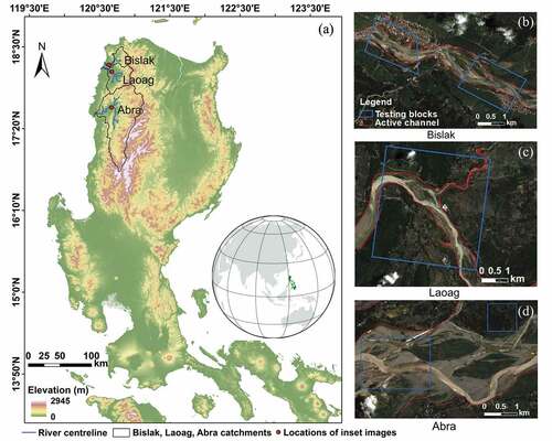
The study area in northwest Luzon, the Philippines, experiences frequent tropical storms and cyclones, which bring heavy precipitation causing landslides and flooding in the region (Faustino-Eslava et al. Citation2013). The area is dominated by a sub-tropical East Asian monsoon climate (Liu et al. Citation2009). In the northwest Philippines, the wet season begins with increased rainfall around May to June and continues until rainfall decreases around October to November (Kubota et al. Citation2017).
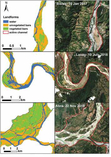
Our investigation focused upon three watercourses in Luzon: the Bislak, Laoag and Abra Rivers (). These gravel-bed rivers are all characterised by planforms that include water, unvegetated bars and vegetated bars/islands. Relating to the spatial resolution of the satellite imagery available for analysis, image processing focused on sufficiently wide sections of the rivers that their morphology could be adequately resolved (Gilvear and Bryant Citation2016). The 39-km-long section of the Bislak River has a mean width (MW) of 375 m; it is the shortest of the three rivers and has relatively small tributary inputs compared to the other two rivers. The 47-km-long section of the Laoag River has a MW of 580 m and has three approximately equally sized tributaries, whose MW varies from 237 m to 424 m. The Abra River (MW: 2441 m, 82 km section length) has three main tributaries; one large tributary has a MW of 1804 m and has extensive agricultural development within the active channel.
Figure 1. (a) Study area showing locations of the (b) Bislak, (c) Laoag and (d) Abra Rivers in northwest Luzon, the Philippines.
3. Datasets and methods
3.1. Sentinel-2 imagery and ground truth digitisation
Sentinel-2 provides imagery with 13 multispectral bands varying from 10 m to 60 m resolution and data availability since 23 June 2015. In this study, Sentinel-2 imagery acquired between January 2017 and December 2019 were analysed. Data were accessed through the USGS Earth Explorer Portal (https://earthexplorer.usgs.gov/; ). A cloud-free Sentinel-2 image (with very small proportion of haze clouds) acquired on 1 January 2018, under growing vegetation and low water flow conditions, was initially used to develop a manually digitised ground truth map of landforms in the Bislak River (water: 1.93 km2, unvegetated bars: 6.28 km2, vegetated bars: 6.15 km2). The ground truth map was used to assess the results from the three approaches to downscaling. To train and validate a multi-temporal model, Sentinel-2 acquisitions of the Bislak River for six dates in 2018 were selected for digitisation. To test the transferability of the multi-temporal Bislak training model to other years, Sentinel-2 acquisitions on six dates in both 2017 and 2019 were used. To test the transferability of the training model to other nearby rivers, Sentinel-2 acquisitions of the Laoag River on six dates in 2018 and of the Abra River on six dates in 2019 were used.
Table 1. Sentinel-2 acquisition dates for each river from 2017 to 2019.
3.2. Image pre-processing
The L1C image datasets were atmospherically corrected using Sen2Cor within the ESA SNAP software. Bands with 10 m and 20 m resolution were used to build the machine learning model. In this case, bands at 20 m resolution were processed to 10 m resolution using three downscaling approaches: super-resolution (Brodu Citation2017), ATPRK (Wang et al. Citation2016) and nearest neighbour resampling. The super-resolution approach used in this study was directly achieved by the Sen2Res tool in SNAP (version 7.0). The nearest neighbour resampling was also performed in SNAP while the ATPRK approach was run in MATLAB R2019a.
In addition to the Sentinel-2 bands, five environmental indices () were generated and incorporated into the machine learning model, resulting in a total of 15 features (10 multi-spectral bands and 5 environmental indices) for the river landform classification.
Table 2. Selected indices for classification.
3.3. Geographic Object Based Image Analysis (GEOBIA)
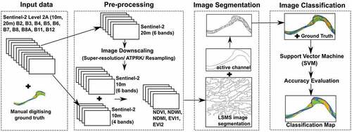
GEOBIA was employed for image segmentation and classification. The Large-Scale Mean Shift (LSMS) algorithm in Orfeo Toolbox (version 6.6.1) was used for the segmentation of objects within the river channel. Three landforms within the river were defined by manually digitising water, unvegetated bars and vegetated bars. The objects were trained together with the manually digitised ground truth map and input into the Support Vector Machine (SVM) model and subsequently evaluated, following the workflow described in . For the SVM model, a regularisation parameter of 1.0 and a scale radial basis function kernel were used and implemented using scikit-learn in Python 3.7.
Figure 2. Workflow for river landform classification.
3.4. Downscaling choice
Sentinel-2 images for the Bislak River on 1 January 2018 were used to compare the three downscaling approaches. In this case, the Bislak River was firstly divided into 10 blocks, using a 7:3 split for training and testing blocks. The numbers of training and testing objects are given in Table A1. Image processing efficiency and classification performance were assessed for all of the three approaches (). The classification accuracy of each dataset was evaluated using the overall accuracy, precision, recall and F1-score. Per-class accuracies (water accuracy (WA), unvegetated bar accuracy (BA) and vegetated bar accuracy (VA)) were also considered.
3.5. Optimal training model
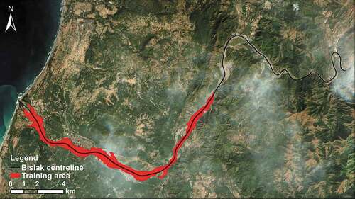
To investigate an optimal machine learning model, both the training and testing data selections were considered. This study started landform classification using a single-date model (for both training and testing datasets) and a six-date model (for both training and testing datasets). In this case, the training model () generated on 1 January 2018 was initially set (Table A2), and then tested on the whole reach (red extent of ) for the remaining five dates in 2018. In this experiment, the ‘unknown units’ (e.g. urban structures, cloud and shadows), were named as ‘others’ and incorporated in the training model. To gain a better understanding of the classification performance of unknown units, the testing site from 10 July 2018, which is partly covered by clouds, was extended by 20 m outside the active channel boundary to incorporate urban pixels. In this way, a mixed group of ‘others’ was prepared for testing.
Figure 3. Selected imagery extent for building optimal training model in the Bislak River. Background is the true colour Sentinel-2 image dated 1 January 2018.
Consequently, a modified approach was conducted on a new group of training and testing datasets. Firstly, a 19 km reach of the Bislak River () was selected as the experimental area within which 10 sub-reaches were established, given serial numbers and allocated to either training or testing datasets ().
Figure 4. Ten sub-reaches of the Bislak River experimental area with serial number. Background is the true colour Sentinel-2 image dated 1 January 2018.
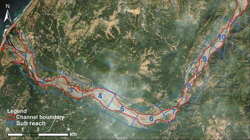
The training dataset (Table A3) was combined by objects from blocks 1, 2, 4, 6, 7 and 10 for six dates in 2018 (1 January, 7 March, 1 May, 20 July, 18 September, 7 November). In this case, we added the class ‘others’, which incorporate unknown objects (occupying 1.1% of the data). With the SVM algorithm, the training model was established and validated on the objects from blocks 3, 5, 8 and 9 (; partly shown in ) of the same dates. Furthermore, imagery observations indicate that three landform types (water, unvegetated bar and vegetated bar) are always present and change locations within blocks 3 and 5 in different seasons. To assess the general performance of the machine learning model for different years, the training model was tested on the objects from blocks 3 and 5 of the Bislak River in 2017 and 2019 (Table A3). We avoided blocks that were obscured by clouds.
3.6. Optimal testing dataset
To investigate the performance of different testing datasets, three combinations of segmented objects were explored: (i) river objects from one single date; (ii) river objects from six dates in a year, including heavy cloud cover dates (over 30% cloud covering the studied river); and (iii) river objects from four less cloudy (under 30%) dates in a year. Thus, in this section, the training dataset consisted of 7458 objects from the 10 Bislak sub-reaches of every two months (6 months in total) in 2018, including ‘water’, ‘unvegetated bar’, ‘vegetated bar’ and ‘others’. To identify an optimal testing dataset, three forms of data tests were designed and applied to the machine learning model. Firstly, the training model was tested on channel objects from single dates in 2017 and testing accuracies were calculated. Secondly, the training model was tested on all channel objects of six dates in 2017, including days with heavy cloud cover (≥30%) acquisitions. Lastly, the training model was tested on all channel objects from four dates in 2017, representing the less cloudy (<30%) acquisitions. Blocks 3 and 5 in (see Table A3) were extracted for the accuracy assessment. The classification performance was compared between the three testing scenarios and an optimal testing dataset was selected for further landform classification analysis. The machine learning model was then applied to the Laoag and Abra Rivers to investigate the transferability of the model. The testing sub-reaches of these rivers are shown in .
4. Results and discussion
4.1. Comparison of downscaling approaches
shows a sample of the segmentation results. The 20 m resolution bands of Sentinel-2 were downscaled to 10 m resolution using the Sen2Res based super-resolution approach, ATPRK, and nearest neighbour resampling. The LSMS segmentation algorithm was subsequently employed to segment the composite bands processed by each approach into objects. The range radius and minimum segment size for the super-resolution approach shows a large difference compared to both resampling and ATPRK methods. Specifically, the super-resolution approach requests only 1 minimum segment size for delineating the channel landforms well, while the resampling and ATPRK methods use 42 minimum segment sizes to differentiate the objects within the channel. The minimum segment size refers to the criterion that is set for merging adjacent small segments with the closest spectral signature after segmentation. Thus, different choices of parameters lead to different sizes of segmented objects. Moreover, the different segmentation procedures result in datasets of varying sizes at the same spatial extent, with super-resolution capturing 154,841 objects after segmentation, resampling retrieving 1077 objects, and ATPRK retrieving 1068 objects.
Figure 5. Sample of segmentation results for (a) super-resolution, (b) resampling and (c) ATPRK. Segmented Objects are categorized by red boundaries. Background images are the composite of band 5 (central wavelength: 704.1 nm), band 6 (central wavelength: 740.5 nm) and band 7 (central wavelength: 782.8 nm) of downscaled Sentinel-2 images dated 1 January 2018.
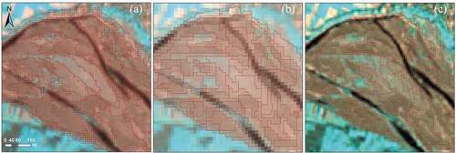
The subsequent classification performances for the three approaches designed in section 3.4 are displayed in . The ATPRK classification performed best among the three methods. However, in this case, the methods were compared at different object scales (minimum segment sizes are varying between the three approaches, see ). To fit a common ground truthing to the segmented objects well, the minimum segment size of image objects with ATPRK and resampling approaches were chosen as much larger than that from the super-resolution approach. This means that segments from ATPRK and resampling images preserved more spatial geometric information since it is easier to find similar adjacent segments to represent spatial features. This might be explained by prior geometric interruptions of the super-resolution method, which was introduced in section 1. Classification of water areas based on resampling implied that the misclassified water bodies always occur in narrow channels, whilst ATPRK performed well in these narrow channels. This result is expected, given the difference between the expected spatial detail interpretation from ATPRK and the resampling methods, explained in section 1. This initial experiment provided a first overall comparison of the three downscaling approaches for classification of the Bislak River’s landforms. The results indicate that the image downscaling approaches can be essential to process object-based classification using Sentinel-2 imagery. The results show that the ATPRK method can outperform the other approaches in rivers of the type found in this region. While resampling performs slightly better than ATPRK for the unvegetated bar and vegetated bar classification accuracies, when it comes to spatial details, the water accuracy is only approximately half that of ATPRK. Thus, the ATPRK approach was used to address research questions 2 to 4.
Table 3. Accuracy assessments for resampling, ATPRK and super-resolution approaches. (All values range between 0–1, whereby 0 indicates the lowest accuracy and 1 indicates the highest accuracy).
4.2. Training model investigation
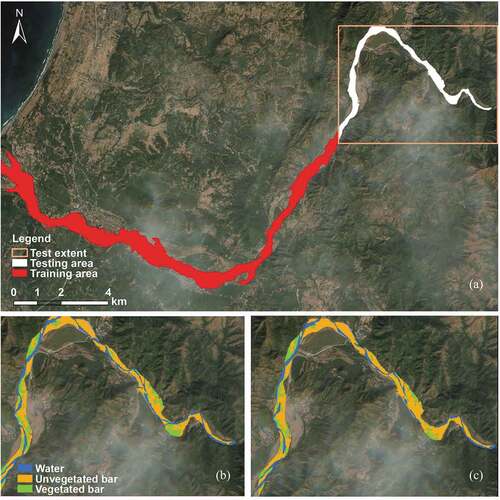
To determine the robustness of the training model based on 1 January 2018 data, the objects of the whole reach were used as a training dataset ( red extent) and the model tested on a different reach ( white extent), located farther upstream in the catchment with fewer unknown objects (e.g. clouds and urban units). The cross-validation accuracy of the model was 0.91 and the test accuracy for this upstream reach was 0.929. The accuracy of water classification was 0.891, unvegetated bars was 0.941 and vegetated bars was 0.940. Generally, the whole test accuracy is close to the validation accuracy, and the classifier performed well for classifying the landforms in the upstream reach on 1 January 2018.
Figure 6. Classification on an upstream reach of the Bislak River; (a) is the true colour Sentinel-2 image with training and testing area, (b) is the manually digitised ground truth representing white extent in (a), and (c) is the output classification. Background image is the true colour Sentinel-2 image dated 1 January 2018.
To investigate the training model (red extent in ) performance across a broader temporal scale, five acquisitions over the Bislak River between 7 March 2018 and 7 November 2018 were selected for testing. displays the accuracies across all dates. It can be seen from that the 1 January 2018 training model does not perform well for all dates in 2018. The training model developed in the dry season fitted March and November images very well, both of which are in the dry season. The testing result was good (overall accuracy is 0.85) on 1 May 2018, which is a transition period between the dry and wet seasons. The 18 September had the poorest performance, which is at the end of the wet season. At this time in the year, it is likely that vegetation growth and suspended sediment load contribute to changes in the spectral properties of vegetated bars and water (Welber, Bertoldi, and Tubino Citation2012). In addition to water, unvegetated bars and vegetated bars, we incorporated a very small proportion (2%) of unknown units, which were named ‘others’, into the training model in this experiment. We tested performance using objects from 10 July 2018, including 308 objects defined as ‘others’. Most objects in this category are urban structures aligned with the active channel of the river, and some are clouds or cloud shadows. The results showed that only 7 objects were misclassified (accuracy is 0.98), which implies the ‘unknown units’ are not the cause of low accuracies on 10 July 2018. Rather, these low accuracies are probably caused by the lack of a seasonal consideration in the training model. Thus, establishing an optimal training model for the research area should incorporate acquisitions across different periods during both the dry and wet seasons.
Table 4. Accuracies on different dates in 2018 using training model from single date. (All values range between 0 and 1, whereby 0 indicates the lowest accuracy and 1 indicates the highest accuracy.).
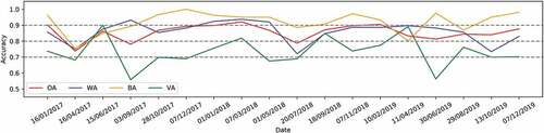
Consequently, the new modified training model established on sub-reaches across different seasons in 2018 was designed and tested on objects of different dates from 2017 to 2019 (Table A3). combines the testing accuracies based on dates across the three years. The overall accuracy for the model is mostly between 0.80 and 0.90. The best classified unit is unvegetated bar (most accuracies ≥0.90) and the poorest classified unit is vegetated bar (accuracies vary between 0.54 and 0.91). Water can generally be well classified (accuracies mostly above 0.80) except for a few dates. These observations demonstrated that using data from multiple dates in constructing the training model can lead to performance that is superior to a single-date training model.
Figure 7. Time series for the testing accuracy of the multi-temporal training model across three years (2017–2019).
4.3. Testing dataset selection
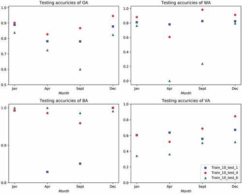
We investigated testing datasets for establishing an optimum machine learning model for river landform classification in the region. From the results presented in section 4.2, a multi-date training model is more favourable for local channel landform classification. Thus, we used a multi-date training model (section 3.5) to run testing to define an optimal testing dataset. The method has been described in section 3.6 and the test experiment accuracies are displayed in . In general, the training model on 10 blocks in and tested on objects of four cloud-free dates (Train_10_test_4) contributes the best performance for the river landform classification. This model performed best for water and vegetated bars except in April 2017, when a single date testing dataset provided higher accuracies. However, for unvegetated bar units, the single date testing dataset obtained much lower accuracies compared to the multi-date testing dataset (including both heavy clouds and less clouds datasets) in April and September 2017. However, in the case of unvegetated bar units, the heavy cloud-based testing dataset performs slightly better than the dataset with less cloud. The testing results for unvegetated bars may be explained by the low water extent and high sediment exposure in the dry season. Additionally, most mis-classified vegetation objects were classified as unvegetated bars (see ), which is likely related to there being sparse vegetation in these objects. From results in this section, we suggest that considering the format of the testing dataset could help when deriving different objective classification results. To pursue an overall high accuracy classification when unvegetated bars are the dominant river landform, we recommend using a multi-date, low cloud cover dataset to define the classification. Moreover, to study landform change in a season which is very short or that shows difference from the whole year, such as April in this case, a testing dataset from a single date might be more effective.
Figure 8. Comparisons of three testing datasets evaluated by overall accuracy (OA), water accuracy (WA), unvegetated bar accuracy (BA) and vegetated bar accuracy (VA). Train_10_test_1 refers to the training model based on ten blocks in Figure 4 and tested on single dates in 2017. Train_10_test_4 refers to the training model based on ten blocks in Figure 4 and tested on four dates in 2017, representing less cloudy acquisitions. Train_10_test_6 refers to the training model based on ten blocks in Figure 4 and tested on six dates in 2017, including dates with heavy cloud cover.
4.4. Model performance in nearby rivers
To explore the transferability of the developed machine learning model, further testing was performed in two nearby rivers: the Laoag and Abra Rivers. For the Laoag River, object samples from six cloud-free acquisitions in 2018 () were collected for model testing. The total number of testing samples in the Laoag River is 2037 (training: testing ≈10:3). For the Abra River, object samples from six cloud-free acquisitions in 2019 () had 2424 testing samples in total (training: testing ≈10:4). and . show the test accuracies for the Laoag River in 2018 and Abra River in 2019, respectively. Here, we used a multi-date testing dataset to run the classification.
Table 5. Test accuracies of the Laoag River in 2018. (All values range between 0 and 1, whereby 0 indicates the lowest accuracy and 1 indicates the highest accuracy).
Table 6. Test accuracies of the Abra River in 2019. (All values range between 0 and 1, whereby 0 indicates the lowest accuracy and 1 indicates the highest accuracy).
These results indicate that, for the whole year, the overall accuracies, water accuracies, and unvegetated bar accuracies within nearby rivers are equal or above 0.86, while vegetated bar accuracies are equal or below 0.735. Specifically, the vegetation accuracies of 10 July 2018 on the Laoag River, and 11 January 2019 on the Abra River are lower than 0.600. This lower accuracy is related to the low proportion of vegetated objects within the testing sub-reaches, which enhance the misclassification. Finer resolution remote sensing data might help to improve the vegetation accuracy for low or sparsely vegetated areas (Huylenbroeck et al. Citation2020). Most mis-classified vegetation objects were classified as unvegetated bars, and notably, the unvegetated bar classification performance is good (>0.812) across all dates of both rivers. The machine learning model can be regarded as reasonably robust across the different rivers and is subsequently applied to further Sentinel-2 images to generate a dataset of river patterns within the region ().
Figure 9. Subset classification results of the Bislak, Laoag and Abra Rivers across different times of different years. Complete classification coverages can be accessed from the link in the Data Availability section.
5. Conclusions
This investigation shows the ATPRK approach to downscaling outperforms the alternatives of nearest neighbour resampling and super-resolution for river landform classification. A new image processing workflow for the purpose of river landform classification was developed and tested across tropical rivers in the Philippines. We also demonstrated that using a multi-temporal dataset across seasons to build a training model is superior to single-date and single-season models. We recommend using testing data at similar temporal ranges to train data and achieve higher classification accuracy. Whilst the scale between ground truth mapping and image segmented objects could impact classification accuracy, our set of experiments (during image pre-processing, downscaling, segmentation, classification) demonstrate optimal data/image processing and river landform classification modes to improve the classification performance. The results show that the proposed workflow can be used for river landform classification across three neighbouring catchments, and it is possible that the training model could successfully be applied to other tropical rivers in the Philippines and beyond with similar hydro-geomorphological characteristics.
Data availability
Data are available from : http://dx.doi.org/10.5525/gla.researchdata.1355.
TableA3_revision.pdf
Download PDF (23.5 KB)TableA2_revision.pdf
Download PDF (15 KB)TableA1_revision.pdf
Download PDF (13.2 KB)Acknowledgements
We would like to thank the two anonymous reviewers and Associate Editor whose comments helped us to improve our manuscript.
Disclosure statement
The authors declare that they have no known competing financial interests or personal relationships that could have appeared to influence the work reported in this paper.
Supplementary material
Supplemental data for this article can be accessed online at https://doi.org/10.1080/01431161.2022.2139164
Additional information
Funding
References
- Bangira, T., S. M. Alfieri, M. Menenti, and A. van Niekerk. 2019. ”Comparing Thresholding with Machine Learning Classifiers for Mapping Complex Water.” Remote Sensing 11 (11): 1351. ARTN 1351. doi:10.3390/rs11111351.
- Boothroyd, R. J., R. D. Williams, T. B. Hoey, B. Barrett, and O. A. Prasojo. 2021. ”Applications of Google Earth Engine in Fluvial Geomorphology for Detecting River Channel Change”. Wiley Interdisciplinary Reviews-Water 8(1). ARTN e21496. doi:10.1002/wat2.1496.
- Brodu, N. 2017. “Super-Resolving Multiresolution Images with Band-Independent Geometry of Multispectral Pixels.” IEEE Transactions on Geoscience and Remote Sensing 55 (8): 4610–4617. doi:10.1109/TGRS.2017.2694881.
- Carbonneau, P. E., B. Belletti, M. Micotti, B. Lastoria, M. Casaioli, S. Mariani, G. Marchetti, and S. Bizzi. 2020. “UAV-Based Training for Fully Fuzzy Classification of Sentinel-2 Fluvial Scenes.” Earth Surface Processes and Landforms 45 (13): 3120–3140. doi:10.1002/esp.4955.
- Carlson, T. N., and D. A. Ripley. 1997. “On the Relation Between NDVI, Fractional Vegetation Cover, and Leaf Area Index.” Remote Sensing of Environment 62 (3): 241–252. doi:10.1016/S0034-4257(97)00104-1.
- Daryaei, A., H. Sohrabi, C. Atzberger, and M. Immitzer. 2020. ”Fine-Scale Detection of Vegetation in Semi-Arid Mountainous Areas with Focus on Riparian Landscapes Using Sentinel-2 and UAV Data.” Computers and Electronics in Agriculture 177: 105686. doi:10.1016/j.compag.2020.105686, ARTN 105686.
- Del Rio-Mena, T., L. Willemen, G. T. Tesfamariam, O. Beukes, and A. Nelson. 2020. ”Remote Sensing for Mapping Ecosystem Services to Support Evaluation of Ecological Restoration Interventions in an Arid Landscape.” Ecological Indicators 113: 106182. doi:10.1016/j.ecolind.2020.106182, ARTN 106182.
- Demarchi, L., S. Bizzi, and H. Piegay. 2016. ”Hierarchical Object-Based Mapping of Riverscape Units and In-Stream Mesohabitats Using LiDar and VHR Imagery.” Remote Sensing 8 (2): 97. ARTN 97. doi:10.3390/rs8020097.
- Faustino-Eslava, D. V., C. B. Dimalanta, G. P. Yumul, N. T. Servando, and N. A. Cruz. 2013. “Geohazards, Tropical Cyclones and Disaster Risk Management in the Philippines: Adaptation in a Changing Climate Regime.” Journal of Environmental Science and Management 16 (1): 84–97. doi:10.47125/jesam/2013_1/10.
- Freitas, P., G. Vieira, J. Canario, D. Folhas, and W. F. Vincent. 2019. “Identification of a Threshold Minimum Area for Reflectance Retrieval from Thermokarst Lakes and Ponds Using Full-Pixel Data from Sentinel-2.” Remote Sensing 11 (6): ARTN 657. doi:10.3390/rs11060657.
- Gao, B. C. 1996. “NDWI - a Normalized Difference Water Index for Remote Sensing of Vegetation Liquid Water from Space.” Remote Sensing of Environment 58 (3): 257–266. doi:10.1016/S0034-4257(96)00067-3.
- Gilvear, D., and R. Bryant. 2016. “Analysis of Remotely Sensed Data for Fluvial Geomorphology and River Science.” In Tools in Fluvial Geomorphology, 103–132.
- Gurnell, A. 2014. “Plants as River System Engineers.” Earth Surface Processes and Landforms 39 (1): 4–25. doi:10.1002/esp.3397.
- Hohensinner, S., G. Egger, S. Muhar, L. Vaudor, and H. Piegay. 2021. “What Remains Today of Pre-Industrial Alpine Rivers? Census of Historical and Current Channel Patterns in the Alps.” River Research and Applications 37 (2): 128–149. doi:10.1002/rra.3751.
- Huete, A., K. Didan, T. Miura, E. P. Rodriguez, X. Gao, and L. G. Ferreira. 2002. ”Overview of the Radiometric and Biophysical Performance of the MODIS Vegetation Indices.” Remote Sensing of Environment 83 (1–2): 195–213. doi:10.1016/S0034-4257(02)00096-2.
- Huylenbroeck, L., M. Laslier, S. Dufour, B. Georges, P. Lejeune, and A. Michez. 2020. ”Using Remote Sensing to Characterize Riparian Vegetation: A Review of Available Tools and Perspectives for Managers.” Journal of Environmental Management 267: 110652. doi:10.1016/j.jenvman.2020.110652, ARTN 110652.
- Jiang, Z. Y., A. R. Huete, K. Didan, and T. Miura. 2008. “Development of a Two-Band Enhanced Vegetation Index Without a Blue Band.” Remote Sensing of Environment 112 (10): 3833–3845. doi:10.1016/j.rse.2008.06.006.
- Korhonen, L., P. P. Hadi, M. Rautiainen, and M. Rautiainen. 2017. “Comparison of Sentinel-2 and Landsat 8 in the Estimation of Boreal Forest Canopy Cover and Leaf Area Index.” Remote Sensing of Environment 195: 259–274. doi:10.1016/j.rse.2017.03.021.
- Kuan, H. F., J. Li, X. J. Zhang, J. P. Zhang, H. Cui, and Q. Sun. 2020. ”Remote Estimation of Water Quality Parameters of Medium- and Small-Sized Inland Rivers Using Sentinel-2 Imagery.” Water 12 (11): 3124. ARTN 3124. doi:10.3390/w12113124.
- Kubota, H., R. Shirooka, J. Matsumoto, E. O. Cayanan, and F. D. Hilario. 2017. ”Tropical Cyclone Influence on the Long-Term Variability of Philippine Summer Monsoon Onset.’ Progress in Earth and Planetary Science 4: ARTN 27 10.1186/s40645-017-0138-5.
- Lanaras, C., J. Bioucas-Dias, S. Galliani, E. Baltsavias, and K. Schindler. 2018. “Super-Resolution of Sentinel-2 Images: Learning a Globally Applicable Deep Neural Network.” Isprs Journal of Photogrammetry and Remote Sensing 146: 305–319. doi:10.1016/j.isprsjprs.2018.09.018.
- Laso, F. J., F. L. Benitez, G. Rivas-Torres, C. Sampedro, and J. Arce-Nazario. 2020. ”Land Cover Classification of Complex Agroecosystems in the Non-Protected Highlands of the Galapagos Islands.” Remote Sensing 12 (1): 65. ARTN 65. doi:10.3390/rs12010065.
- Liu, Z. F., Y. L. Zhao, C. Colin, F. P. Siringan, and Q. Wu. 2009. “Chemical Weathering in Luzon, Philippines from Clay Mineralogy and Major-Element Geochemistry of River Sediments.” Applied Geochemistry 24 (11): 2195–2205. doi:10.1016/j.apgeochem.2009.09.025.
- Mandarino, A., M. Maerker, and M. Firpo. 2019. “Channel Planform Changes Along the Scrivia River Floodplain Reach in Northwest Italy from 1878 to 2016.” Quaternary Research 91 (2): 620–637. doi:10.1017/qua.2018.67.
- Maxwell, A. E., T. A. Warner, and F. Fang. 2018. “Implementation of Machine-Learning Classification in Remote Sensing: An Applied Review.” International Journal of Remote Sensing 39 (9): 2784–2817. doi:10.1080/01431161.2018.1433343.
- Phiri, D., M. Simwanda, S. Salekin, V. R. Nyirenda, Y. Murayama, and M. Ranagalage. 2020. ”Sentinel-2 Data for Land Cover/Use Mapping: A Review.” Remote Sensing 12 (14): 2291. ARTN 2291. doi:10.3390/rs12142291.
- Roy, D. P., and O. Dikshit. 1994. “Investigation of Image Resampling Effects Upon the Textural Information-Content of a High-Spatial-Resolution Remotely-Sensed Image.” International Journal of Remote Sensing 15 (5): 1123–1130. doi:10.1080/01431169408954146.
- Selva, M., B. Aiazzi, F. Butera, L. Chiarantini, and S. Baronti. 2015. “Hyper-Sharpening: A First Approach on SIM-GA Data.” Ieee Journal of Selected Topics in Applied Earth Observations and Remote Sensing 8 (6): 3008–3024. doi:10.1109/Jstars.2015.2440092.
- Serlet, A. J., A. M. Gurnell, G. Zolezzi, G. Wharton, P. Belleudy, and C. Jourdain. 2018. “Biomorphodynamics of Alternate Bars in a Channelized, Regulated River: An Integrated Historical and Modelling Analysis.” Earth Surface Processes and Landforms 43 (9): 1739–1756. doi:10.1002/esp.4349.
- Sonobe, R., Y. Yamaya, H. Tani, X. F. Wang, N. Kobayashi, and K. Mochizuki. 2018. ”Crop Classification from Sentinel-2-Derived Vegetation Indices Using Ensemble Learning.” Journal of Applied Remote Sensing 12 (2): 1. Artn 026019. doi:10.1117/1.Jrs.12.026019.
- Spada, D., P. Molinari, W. Bertoldi, A. Vitti, and G. Zolezzi. 2018. ”Multi-Temporal Image Analysis for Fluvial Morphological Characterization with Application to Albanian Rivers.” Isprs International Journal of Geo-Information 7 (8): 314. ARTN 314. doi:10.3390/ijgi7080314.
- Vargas-Luna, A., G. Duro, A. Crosato, and W. Uijttewaal. 2019. “Morphological Adaptation of River Channels to Vegetation Establishment: A Laboratory Study.” Journal of Geophysical Research-Earth Surface 124 (7): 1981–1995. doi:10.1029/2018jf004878.
- Wang, Q. M., W. Z. Shi, P. M. Atkinson, and Y. L. Zhao. 2015. “Downscaling MODIS Images with Area-To-Point Regression Kriging.” Remote Sensing of Environment 166: 191–204. doi:10.1016/j.rse.2015.06.003.
- Wang, Q. M., W. Z. Shi, Z. B. Li, and P. M. Atkinson. 2016. “Fusion of Sentinel-2 Images.” Remote Sensing of Environment 187: 241–252. doi:10.1016/j.rse.2016.10.030.
- Welber, M., W. Bertoldi, and M. Tubino. 2012. “The Response of Braided Planform Configuration to Flow Variations, Bed Reworking and Vegetation: The Case of the Tagliamento River, Italy.” Earth Surface Processes and Landforms 37 (5): 572–582. doi:10.1002/esp.3196.
- Yang, X. C., S. S. Zhao, X. B. Qin, N. Zhao, and L. G. Liang. 2017. ”Mapping of Urban Surface Water Bodies from Sentinel-2 MSI Imagery at 10 M Resolution via NDWI-Based Image Sharpening.” Remote Sensing 9 (6): 596. ARTN 596. doi:10.3390/rs9060596.
- Zheng, H. R., P. J. Du, J. K. Chen, J. S. Xia, E. Z. Li, Z. G. Xu, X. J. Li, and N. Yokoya. 2017. ”Performance Evaluation of Downscaling Sentinel-2 Imagery for Land Use and Land Cover Classification by Spectral-Spatial Features.” Remote Sensing 9 (12): 1274. ARTN 1274. doi:10.3390/rs9121274.