Almond cultivar identification using machine learning classifiers applied to UAV-based multispectral data

ABSTRACT

In Portugal, almonds are a very important crop, due to their nutritional properties. In the northeastern part of the country, the almond sector has endured over time, with strong cultural traditions and key economic significance. In these areas, several cultivars are used. In effect, the presence of various almond cultivars implies differentiated management in irrigation, disease control, pruning system, and harvest planning. Therefore, cultivar classification is essential over large agricultural areas. Over the last decades, remote-sensing data have led to important breakthroughs in the classification of different cultivars for several crops. Nonetheless, for almonds, studies are incipient. Thus, this study aims to fill this knowledge gap and explore the classification of almond cultivars in an almond orchard. High-resolution multispectral data were acquired by an unmanned aerial vehicle (UAV). Vegetation indices (VIs) and tree structural parameters were, subsequently, estimated. To obtain an accurate cultivar identification, four machine learning classifiers, such as K-nearest neighbour (kNN), support vector machine (SVM), random forest (RF), and extreme gradient boosting (XGBoost), were applied and optimized through the fine-tuning process. The accuracy of machine learning classifiers was analysed. SVM and RF performed best with OAs of 76% and 74% using VIs and spectral bands (GREEN, GRVI, GN, REN, ClRE). Adding the canopy height model (CHM) improved performance, with RF and XGBoost having OAs of 88% and 84%. kNN performed worst with an OA of 73% using only VIs and spectral bands, 80% with VIs, spectral bands and CHM, and 93% with VIs, CHM, and tree crown area (TCA). The best performance was achieved by RF and XGBoost with OAs of 99% using VIs, CHM, and TCA. These results demonstrate the importance of the feature selection process. Moreover, this study reveals the feasibility of remote-sensing data and machine learning classifiers in the classification of almond cultivars.

KEYWORDS:

• unmanned aerial vehicles
• precision agriculture
• Prunus dulcis
• tree cultivars classification
• K-nearest neighbour
• support vector machine
• random forest
• extreme gradient boosting

1. Introduction

Prunus Dulcis (Mill. D. A. Webb), commonly known as almond, is an extremely valuable commercial crop, particularly due to its beneficial nutritional properties (Sumner et al. 2016). California (United States of America) is the most important production region worldwide, accounting for roughly 60% of global supply. Global almond production is increasing, particularly in Mediterranean countries such as Portugal, Spain, Italy, and France, where a dry and hot climate is ideal for almond development (Pathak, Maskey, and Rijal 2021; Rodrigues, Venâncio, and Lima 2012). In Portugal, almond crops are essentially located in the regions of Trás-os-Montes, Alentejo, and Algarve (Soares et al. 2012), where the recent production increases have been accompanied by shifts from traditional/native to more suitable almond cultivars. These cultivars are more climatically adapted and exhibit late flowering, contributing to increased production levels (Egea et al. 2003). Lauranne and Francolí, are two varieties that stand out as particularly profitable and productive cultivars, widely used in almond production countries (Miarnau, Alegre, and Vargas 2010). Lauranne was created by the National Institute of Agricultural Research (INRA) of Avignon, in 1978, as a result of a cross (‘Ferragnes’ x ‘Tuono’), while Francolí was created by the Institute of Agrifood Research and Technology (IRTA) of Cataluña, in 1976, as a result of a cross (‘Cristomorto’ × ‘Tuono’) (de Herralde et al. 2001). Although these almond cultivars appear to be quite similar, they reveal distinct characteristics, namely in flowering and harvest periods, vegetative vigour, yield levels, and the requirements of the pruning system. According to Cordeiro et al. (2005), which compares different almond cultivars, Lauranne is the most productive with 5 kg/plant of nuts and Francolí is the most vigorous, with 81 mm in trunk diameter. To manage this variability and benefit from the precision agriculture procedures, it is crucial to distinguish the several cultivars within the crops (Mavridou et al. 2019). The presence of several cultivars implies differentiated management in terms of irrigation needs, phytosanitary control, pruning architecture, and harvesting (Mateo-Aroca et al. 2019; Daponte et al. 2019).

The identification of different tree species and crop cultivars can be provided by several classification methodologies (Haara and Haarala 2002; Fassnacht et al. 2016). Over the last decades, remote-sensing data have been used for the classification process and to assist crop management (Pinter et al. 2003). Initially, this process relied on manually identifying classes through the visual interpretation of remotely sensed images in geographical information systems (GIS), which is a time-consuming task and prone to human error (Fiorucci et al. 2018). Currently, manual procedures are being gradually replaced by automated classifiers based on artificial intelligence (AI) techniques, which resulted in a reduction of inconsistencies and time savings (Loussaief and Abdelkrim 2016). AI is embedded in a wide variety of areas, including medical research, education, finance, security, manufacturing, and agriculture, where it is used to automate complicated operations in a manner like how humans learn and solve problems. Machine learning (ML) is one of the most relevant subfields of AI, providing the analysis of massive quantities of data (Eli-Chukwu 2019; Jha et al. 2019). Indeed, ML algorithms are becoming widely used as a result of their ability to accurately solve common problems in remote-sensing data analysis such as classification, regression, and segmentation (Ghamisi et al. 2019). Logistic regression (LR) (Taha and Shoufan 2019), Naive Bayes (NB) (Preethi, Brintha, and Yogesh 2021), K-nearest neighbour (kNN) (Dainelli et al. 2021), random forest (RF) (Horning 2010), and support vector machine (SVM) (Kok et al. 2021) are among the most used ML classifiers. Several studies implement ML techniques for tree species and cultivars classification, obtaining high overall accuracy (OA) (Fassnacht et al. 2016). Concerning tree species classification studies, Reid, Ramos, and Sukkarieh (2011) collected data using an RGB sensor coupled to an unmanned aerial vehicle (UAV) to classify three species (Prickly acacia, Parkinsonia, Eucalyptus) using Gaussian Processes (GP), obtaining 89% of OA. Chenari et al. (2017), in turn, used an RGB data and a kNN classifier to identify two tree species (wild pistachio and wild almond) with an OA of 90%. Lisein et al. (2015) used an RF classifier, to classify five forest species (English oak, birch, sycamore maple, common ash, and poplar) using multispectral data and obtained an OA of 61.50%. In contrast to other studies that focused on the classification of forest tree species, Csillik et al. (Csillik et al. 2018) took a different approach, implementing the classification process in a fruit orchard. The authors classified citrus and other crop trees from UAV imagery using a simple Convolutional Neural Network (CNN), achieving an OA of 96.24%. Regarding cultivars classification studies, Avola et al. (Avola et al. 2019) applied 14 vegetation indices (VIs) in olives cultivar recognition, using univariate (ANOVA) and multivariate (principal component analysis – PCA – and linear discriminant analysis – LDA) methodologies. The authors obtained an accuracy of 90.9% with LDA, in the classification of scions of two Italian olive cultivars, Frantoio and Leccino, and failed in more than 68.2% in rootstocks classification. Gomes et al. (2020) proved the suitability of leaf reflectance information in 10 olive varieties classification, obtaining in SVM classifier an OA of 81.73%.

Considering a recent review study by Jafarbiglu and Pourreza (2022), the authors suggest that most remote-sensing applications are limitedly studied in nut orchards, including almonds, generating research opportunities. In this article, a pioneering study is presented based on the automatic classification of two almond cultivars (Lauranne and Francolí) using VIs, spectral bands and structural parameters computed from UAV-based high-resolution multispectral data. For this purpose, four ML classifiers (kNN, SVM, RF, and XGBoost) are evaluated.

2. Materials and methods

2.1. Study area

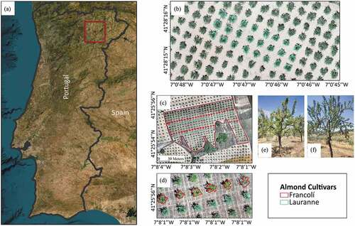
The study was conducted on 29 June 2021 and 4 July 2022 in two rainfed almond orchards with 92 trees. The orchards were located in São Salvador and Bornes in the Mirandela region of Trás-os-Montes, Northeastern Portugal (41°25‘55“ N, 7°08’06‘ W and 41°27“31” N, 7°0’24’ W, respectively, as shown in Figure 1a). The region has a dry, hot climate suitable for almond growth. The study evaluated 47 Francolí cultivar trees from the São Salvador orchard and 45 Lauranne cultivar trees, 23 from São Salvador and 22 from Bornes (Figure 1b, c).

Figure 1. Overview of the studied almond orchards: (a) location of the study areas; (b) almond orchard with Lauranne cultivar, in Bornes; (c) almond orchard with Francolí and Lauranne cultivars, in São Salvador; (d) large-scale image with trees cultivar identification; and photographs of Francolí (e) and Lauranne (f) cultivars.

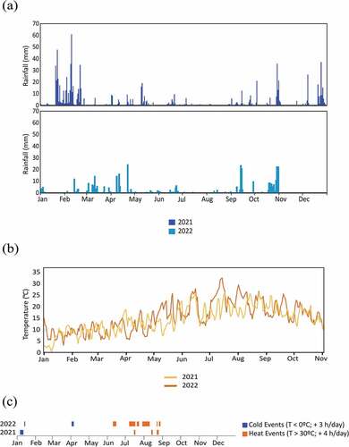
Data collection took place on 29 June 2021 and 4 July 2022 to make the dataset comprehensive, since weather conditions in 2021 differed from those in 2022 (Figure 2a). In 2021, rainfall was higher with 584 mm recorded from January to August, while in 2022 it was only 174 mm (Figure 2b). Compared to the 14-year average of 605 mm, both 2021 and 2022 had lower rainfall. Temperature values in 2022, particularly in summer months, were higher than in 2021 leading to more heat events in 2022 (Figure 2c). These variations led to almond trees in different levels of water stress in the collected data.

Figure 2. Weather conditions in 2021 and 2022. (a) Rainfall values – mm; (b) Temperature values – °C; and (c) cold and heat events.

2.2. UAV data acquisition

Data were collected using a Phantom 4 UAV (DJI, Shenzhen, China), equipped with a CMOS sensor (12.4 Megapixels (MP) resolution), set on a three-axis gimbal to collect georeferenced RGB imagery. The Sequoia multispectral sensor (Parrot SA, Paris, France) was used to capture multispectral imagery. The multispectral sensor can capture four distinct bands with a resolution of 1.2 MP: green (550 nm – 40 nm bandwidth); red (660 nm – 40 nm bandwidth); red edge (735 nm – 10 nm bandwidth); and near-infrared (790 nm – 40 nm bandwidth). Radiometric calibration was performed using the irradiance data collected during the flight, from a sun irradiance sensor, together with images of a specific calibration target. The flight missions were conducted at a flight height of 60 m and with an 80% longitudinal imagery overlap and a 70% lateral overlap, ensuring a good coverage to generate a dense 3D point cloud.

2.3. Data processing

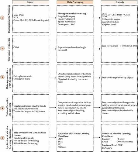
The data processing workflow is divided into five distinct steps that were successively carried out (Figure 3). In step 1, the photogrammetric processing of RGB and multispectral data was performed, obtaining the digital surface model (DSM), digital terrain model (DTM), canopy height model (CHM) (computed by subtracting the DTM from the DSM), orthophoto mosaic and VIs. In step 2 (Tree Crown Delineation), the tree crown mask was created through the segmentation process based on the height threshold applied to the CHM. In step 3 (Data Augmentation – OBIA Segmentation), to divide tree crowns into several objects, the orthophoto mosaic was used to extract objects by applying an object-based image analysis (OBIA) method, and then those are delimited using a tree crown mask. In step 4 (Features Extraction and Labelling), the VIs, spectral bands and structural parameters associated with each tree crown object were extracted. In step 4, the objects of each tree crown were also classified through the labelling process. Lastly, in step 5 (Application of Machine Learning Classifiers), ML classifiers were trained and tested. For these procedures, the labelled dataset was divided, with 70% used for training and 30% used for testing their performance.

Figure 3. Data processing workflow: (1) Photogrammetric processing; (2) Tree crown delineation; (3) Data Augmentation – OBIA segmentation; (4) Features extraction and labelling; (5) Application of machine learning classifiers.

2.3.1. Photogrammetric processing

The UAV imagery, both RGB and multispectral, was subjected to photogrammetric processing (Figure 3 – Step 1), performed in Pix4DMapper Pro (Pix4D SA, Lausanne, Switzerland). This software applies a radiometric calibration of multispectral data and uses the structure for motion (SfM) algorithm to compute the 3-D structure of a scene from a set of images, in other words, a 3D point cloud is derived from the acquired 2D imagery. The images were aligned, based on the detection of common points and the use of ground control points (GCPs). This procedure allowed the generation of several raster outputs, including DSM, DTM, orthophoto mosaic (from the RGB imagery) and VIs (from multispectral imagery). Using QGIS software, the DSM and DTM were used to compute the CHM.

According to the literature, several studies identify the most relevant VIs for tree species and cultivar classification (Avola et al. 2019; Huete et al. 2002; Jafarbiglu and Pourreza 2022). Considering this, a list of several VIs was computed through the photogrammetric processing of multispectral data (Table 1). These VIs were considered during the feature selection process.

Table 1. List of vegetation indices used in cultivar classification and their respective equations.

Name of Index	Equation	Reference
Chlorophyll red-edge index	$\mathrm{C}\mathrm{l}\mathrm{R}\mathrm{E}=\hspace{0.17em}\frac{\mathrm{N}}{\mathrm{R}\mathrm{E}-1}$	(Xu et al., 2021)
Enhanced vegetation index 2	$\mathrm{E}\mathrm{V}\mathrm{I}2=\frac{2.5\hspace{0.17em}\times \hspace{0.17em}\left(\mathrm{N}-\mathrm{R}\right)}{\left(\mathrm{N}+\hspace{0.17em}2.4\hspace{0.17em}\times \mathrm{R}+\hspace{0.17em}1\right)}$	(A. Huete et al. 2002)
Green normalized difference vegetation index	$\mathrm{G}\mathrm{N}\mathrm{D}\mathrm{V}\mathrm{I}=\hspace{0.17em}\frac{\mathrm{N}-\mathrm{G}}{\mathrm{N}+\mathrm{G}}$	(Gitelson et al., 1996)
Green-red vegetation index	$\mathrm{G}\mathrm{R}\mathrm{V}\mathrm{I}=\hspace{0.17em}\frac{\mathrm{G}-\mathrm{R}}{\mathrm{G}+\mathrm{R}}$	(Tucker, 1979)
Normalized difference vegetation index	$\mathrm{N}\mathrm{D}\mathrm{V}\mathrm{I}=\hspace{0.17em}\frac{\mathrm{N}-\mathrm{R}}{\mathrm{N}+\mathrm{R}}$	(Rouse et al., 1974)
Plant senescence reflectance index	$\mathrm{P}\mathrm{S}\mathrm{R}\mathrm{I}=\hspace{0.17em}\frac{\mathrm{R}-\mathrm{G}}{\mathrm{N}}$	(Ren et al., 2017)
Red edge normalized difference vegetation index	$\mathrm{R}\mathrm{E}\mathrm{N}=\hspace{0.17em}\frac{\mathrm{N}-\mathrm{R}\mathrm{E}}{\mathrm{N}+\mathrm{R}\mathrm{E}}$	(Van Beek et al., 2013)
Soil-adjusted vegetation index	$\mathrm{S}\mathrm{A}\mathrm{V}\mathrm{I}=\hspace{0.17em}\frac{\mathrm{N}-\mathrm{R}}{\mathrm{N}+\mathrm{R}+\mathrm{L}}\hspace{0.17em}\times \left(1+\mathrm{L}\right)$	(A. R. Huete, 1988)

N, near infrared; G, reen; R, red; RE, red edge; L, soil-brightness correction.

2.3.2. Tree crown delineation

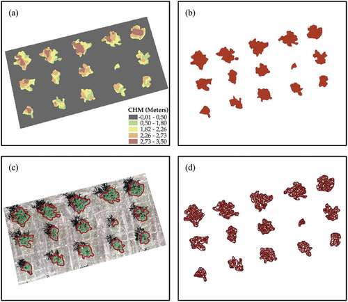
Tree crown delineation is a critical procedure for extracting parameters at the tree level (Pádua et al. 2017), allowing the differentiation of several cultivars. This procedure was implemented considering the methodology applied by Marques et al. (Pedro et al. 2019) and Pádua et al. (2020), where the individual tree crown segmentation (Figure 3 – Step 2) was carried out using the CHM. A threshold of 0.5 m was used during the binarization process since this value was found to be effective in removing all existing lowland vegetation and shadows cast by tree crowns. This procedure originated a binary mask, which was then vectorized to produce the polygons representing each detected tree crown. The procedure depicted in Figure 4 was used to segment tree crowns. During the initial phase, data below 0.5 m of CHM was deleted (Figure 4a). The binarization was then conducted, and only pixels with a height greater than 0.5 m were considered (Figure 4b). Tree crowns were demarcated, removing lowland vegetation and shadows (as shown in Figure 4c). The tree crown delineation process allowed the computation of tree crown area (TCA) parameter.

Figure 4. Tree crown delineation: (a) canopy height model (CHM); (b) binarization process based on CHM threshold (0.5 m); (c) delineation of each tree crown, excluding lowland vegetation and shadows, and (d) object-based image analysis segmentation.

2.3.3. Data augmentation – OBIA segmentation

Data augmentation is frequently used in a wide variety of ML procedures, including image classification. This technique entails increasing the sample size of the training dataset, hence avoiding overfitting issues (Ayan and Murat Ünver 2018). Among data augmentation approaches, this procedure involves flipping, distorting, adding noise, or cutting a patch from the original image (Inoue 2018).

In this study, data augmentation (Step 3 in Figure 3) was performed using an OBIA approach based on the mean shift algorithm (Michel, Youssefi, and Grizonnet 2014), available in the Orfeo ToolBox. This technique was effective to estimate the local density gradients of similar image pixels. Gradient estimation was iteratively conducted for each pixel, allowing the identification of identical neighbouring pixels (Zhou, Wang, and Schaefer 2011). For this study, mean shift algorithm was used with the following parameters – spatial radius: 10 and range radius: 20, applied to the RGB orthophoto mosaic, creating a set of objects (in a vector format), which were delimited by tree crown mask (Figure 4d). After applying this approach, 4932 elements (objects) were created.

2.3.4. Feature extraction and labelling

In the feature extraction and labelling step (Figure 3 – Step 4), VIs, spectral bands and structural parameters, associated with each tree crown object, were extracted by using the raster statistics for polygons tool, provided by System for Automated Geoscientific Analyses (SAGA) GIS. Thus, object feature extraction required computing the mean values of VIs, spectral bands, and structural parameters, considering the information of each pixel contained within the object. A dataset with several features was created.

The application of ML classifiers implied the creation of a target variable (class field) on the dataset to provide information about each almond tree cultivar. Carrying out this process, two labels were created on the class field (Figure 3 – Step 4), to identify the Francolí cultivar (class with label 1) and the Lauranne cultivar (class with label 2).

2.4. Application of machine learning classifiers

Every machine learning project requires the implementation of several procedures, such as data collection and preparation, classifier selection (training and testing), performance evaluation, and hyperparameter tuning.

2.4.1. Data collection and preparation

The data considered in this process were based on VIs, spectral bands, and structural parameters, building a dataset composed of 19 features associated with VIs and spectral bands (ExNIR, ExRE, ClRE, EVI2, NDExNIR, NDExRE, GN, GNDVI, GREEN, GRVI, NDVI, NIR, NIRN, PSRI, RED, REDEDGE, REN, RN, SAVI), as well as two features associated to structural parameters (CHM maximum height and TCA). This dataset was also composed of a target variable, the class, which had labels related to each almond tree cultivar. This dataset contained 7200 samples.

In the initial step of data preparation, the dataset was evaluated to detect missing values, the distribution of each feature, and the existence of outliers. The features in the dataset were also normalized using StandardScaler from Scikit learn python library. After this, coefficients of skewness were determined for each feature, both before and after the outliers removal process. These coefficients measure the distribution’s asymmetries. As shown in Table 2, after removing outliers, asymmetries in coefficients were reduced for most features.

Table 2. Coefficients of skewness for each feature, before and after outliers removal process.

Features	Before outliers removal	After outliers removal
ExNIR	−0.621	−0.410
ExRE	−0.839	−0.695
ClRE	0.948	0.283
EVI2	−0.092	−0.092
NDExNIR	−0.420	−0.306
NDExRE	0.115	−0.249
GN	0.953	0.437
GNDVI	−0.925	−0.537
GREEN	−0.013	−0.034
GRVI	−0.028	−0.028
NDVI	−0.753	−0.663
NIR	−0.169	−0.165
NIRN	−0.420	−0.306
PSRI	1.104	0.763
RED	1.295	0.604
REDEDGE	−0.180	−0.176
REN	0.115	−0.249
RN	0.768	0.702
SAVI	−0.233	−0.233
TCA	0.546	0.223
CHM	−0.504	−0.005

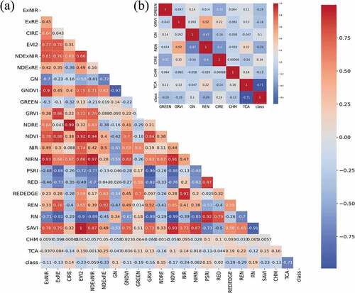
In terms of the features selection method, Pearson’s correlation coefficient was used due to the numerical nature of the features (Figure 5). The feature selection method is essential since it removes irrelevant or redundant data from the dataset (Chandrashekar and Sahin 2014). Considering the heatmap of correlations, represented in Figure 5, seven features were selected (GREEN, GRVI, GN, REN, ClRE, CHM, and TCA). The selection process considered both the most correlated features with the target variable (class) and the lowest correlated features between them.

Figure 5. Heatmap representing the Pearson’s correlation coefficient. (a) All VIs, spectral bands, and structural parameters; (b) Selected features for classification.

2.4.2. Classifier selection – training and testing

Considering the ML classifiers, four different classifiers were implemented: kNN, SVM, RF, and XGBoost (Figure 3 – Step 5). The kNN classifier is a supervised learning technique that can be used for regression as well as classification. By computing the distance between the test data and all the training points, kNN attempts to predict the proper class for the test data. The kNN classifier was chosen due to its simplicity, efficacy, intuitiveness, and competitive classification performance across multiple domains. It is robust to noisy training data and efficient when the training data are considerable (Baf, Im, and Bol 2013). Regarding SVM, it is a supervised machine learning classifier used to analyse data in classification and regression analyses. The SVM classifier identifies a hyperplane in N-dimensional space (N – the number of characteristics) that classifies the data points in a distinct manner (Noble 2006). The selection of SVM classifier for classification is owed to the fact that is consistent with observations that are far from the hyperplane and are efficient since they depend mainly on support vectors within the hyperplane. Moreover, using several kernel functions, SVM can adapt to the nonlinear decision/classification limits and deliver solutions even when the data are not linearly separable. The SVM classifier also presents a better classification performance when applied to unbalanced binary outcome data (Antje and Signorino 2018). The RF classifier, in turn, is a type of ensemble classifier that generates several decision trees from a randomly picked subset of training samples and variables. Due to the accuracy of its classifications, this classifier has gained popularity in the remote-sensing field (Belgiu and Drăguţ 2016). The RF classifier was selected due to its several advantages since it is non-parametric, capable of using continuous and categorical datasets, is simple to parametrize, insensitive to overfitting and computes auxiliary information such as classification loss and feature importance (Horning 2010). XGBoost, on the other hand, was applied since it is a boosting classifier that combines hundreds of tree models with lower classification accuracy, and by constant model iteration, it develops a very accurate and low false positive classifier (Chen et al. 2018).

The machine learning classifiers were applied using Scikit learn. Considering the dataset, 70% of data were used for training (5040 samples) and 30% were used for testing (2160 samples). To ensure that the process is independent of the choice made and to control the overfitting, 10 random dataset train-test splits were defined, with the application of k-folds cross-validation (CV) where dataset was split into k different subsets (or folds).

2.4.3. Classifier performance evaluation

To evaluate the performance of each ML classifier, 30% of testing data were used, producing a confusion matrix (Table 3). In the confusion matrix, the true positive (TP) indicates the number of elements predicted with class 1 that belongs to class 1; the true negative (TN) refers to the number of elements predicted with class 2 that belongs to class 2; the false positive (FP) indicates the number of elements predicted with class 1 that should be predicted as class 2, and the false negative (FN) represents the number of elements predicted with class 2 that should be predicted as class 1.

Table 3. Confusion matrix considering the predicted and true classes.

	Predicted class
	Classes	1	2	Total
True class	1	TP	FN	TP + FN
	2	FP	TN	FP + TN
	Total	TP + FP	FN + TN	TP+FP+FN+TN

TP, true positive; TN, true negative; FP, false positive; FN, false negative.

Several metrics, used in classifiers performance evaluation, can be withdrawn from the confusion table, namely: precision (1), recall (2), f1score (3), and OA (4). Precision quantifies the proportion of units in classifier that are truly positive. In other words, precision indicates the degree to which we may trust a classifier prediction of an individual as positive (Grandini, Bagli, and Visani 2020). Recall quantifies the classifier’s ability to locate all positive units in the dataset (Grandini, Bagli, and Visani 2020). F1-Score evaluates the effectiveness of classification classifiers starting with the confusion matrix; it aggregates Precision and Recall metrics using the harmonic mean approach (Grandini, Bagli, and Visani 2020). OA is a metric that indicates how well the classifier correctly predicts the entire set of data (Grandini, Bagli, and Visani 2020).

The precision-recall – area under the curve (PR AUC) metric was considered in the ML classifiers performance evaluation. PR AUC is a useful metric for determining the success of a prediction when the classes are highly imbalanced (Davis and Goadrich 2006). Additionally, the receiver operating characteristics (ROC) AUC metric was also applied in the evaluation of the classifiers, as it shows the classifiers ability to differentiate between classes (Saito, Rehmsmeier, and Brock 2015). The ROC AUC metric is performed using the true-positive rate (TPR) (2) and the false-positive rate (FPR) (5).

(1) $Precision=\frac{TP}{\left(TP+FP\right)}$(1)

(2) $Recall=TPR=\frac{TP}{\left(TP+FN\right)}$(2)

(3) $F1score=\frac{2\times \left(P\times R\right)}{\left(P+R\right)}\hspace{0.17em}$(3)

(4) $OA=\frac{\left(TP+TN\right)}{\left(TP+TN+FP+FN\right)}\hspace{0.17em}$(4)

(5) $FPR=\frac{FP}{\left(FP+TN\right)}\hspace{0.17em}$(5)

2.4.4. Hyperparameter tuning

The ML classifiers performance is related to hyperparameter configuration. To select the appropriate hyperparameters, users can rely on the default values specified by ML libraries or manually configure them based on the literature, experience, or trial-error method (Probst, Bischl, and Boulesteix 2018). In this study, the hyperparameters were defined based on Scikit learn GridSearchCV method. It combines several hypotheses, identifying the optimal hyperparameters based on the highest performance of ML classifiers. Table 4 shows the hyperparameters considered in the classification process.

Table 4. Main hyperparameters considered during the classification process.

Selected features	Classifier	Tested hyperparameters	Applied hyperparameters
GREEN, GRVI, GN, REN, CIRE	kNN	n_neighbors: range(2, 100, 10)	n_neighbors: 22
	SVM	c: 0.1, 1, 10 kernel: linear, rbf, poly gamma: 0.1, 1, 10	c: 1 kernel: rbf gamma: 1
	RF	n_estimators: range(10, 1000, 10)	n_estimators: 490
	XGBoost	max_depth: 5,10,15,20 min_child_weight: 4, 5, 8 learning_rate: 0.05, 0.1, 0.2 n_estimators: 200, 400, 600, 800	max_depth: 20 min_child_weight: 5 learning_rate: 0.05 n_estimators: 200
GREEN, GRVI, GN, REN, CIRE, CHM	kNN	n_neighbors: range(2, 100, 10)	n_neighbors: 12
	SVM	c: 0.1, 1, 10 kernel: linear, rbf, poly gamma: 0.1, 1, 10	c: 1 kernel: rbf gamma: 1
	RF	n_estimators: range(10, 1000, 10)	n_estimators: 400
	XGBoost	max_depth: 5,10,15,20 min_child_weight: 4, 5, 8 learning_rate: 0.05, 0.1, 0.2 n_estimators: 200, 400, 600, 800	max_depth: 5 min_child_weight: 8 learning_rate: 0.01 n_estimators: 200
GREEN, GRVI, GN, REN, CIRE, CHM, TCA	kNN	n_neighbors: range(2, 100, 10)	n_neighbors: 12
	SVM	c: 0.1, 1, 10 kernel: linear, rbf, poly gamma: 0.1, 1, 10	c: 10 kernel: rbf gamma: 1
	RF	n_estimators: range(10, 1000, 10)	n_estimators: 150
	XGBoost	max_depth: 5,10,15,20 min_child_weight: 4, 5, 8 learning_rate: 0.05, 0.1, 0.2 n_estimators: 200, 400, 600, 800	max_depth: 10 min_child_weight: 4 learning_rate: 0.05 n_estimators: 400

3. Results

According to the methodology implemented, the kNN, SVM, RF, and XGBoost classifiers are applied in almond cultivar classification, using VIs, spectral bands and structural parameters extracted from tree crown objects. In classifiers execution, 10 CV k-folds are performed, using 70% for training (5040 samples) and 30% for testing (2160 samples).

3.1. Feature importance in almond cultivar classification

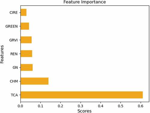
In the RF execution classifier, feature importance scores can demonstrate the significance of each feature in predicting the target variable (Figure 6). In classifiers implementation, five VIs, spectral bands (GREEN, GRVI, GN, REN, ClRE) and two structural parameters (CHM, TCA) are used as features. The TCA feature is the most important predictor of the target variable, as shown in Figure 6. On the other hand, CHM is less significant for predicting the target variable. Regarding VIs and spectral bands, GN, REN, and GRVI are the most relevant predictors. In contrast, GREEN and ClRE features present the lowest importance in the classification process.

Figure 6. Feature importance scores in random forest classifier execution.

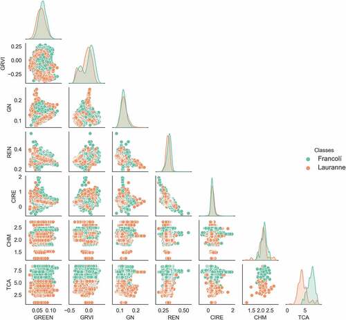
As shown in Figure 7, two classes associated with the target variable (Francolí and Lauranne) exhibit a clear distinction in the TCA feature, which contributes significantly to classification. When TCA is combined with other features, a significant separation in class distribution is also evident. Even though CHM, REN, GN, GREEN, and GRVI features exhibit a slight distinction in class distribution, they also contribute to classification. In contrast, ClRE presents a lower separability in the distribution of classes, indicating that they contribute less to classification.

Figure 7. Distribution of the target variable among the selected classification features. The diagonal graphs show the Kernel Density Estimator (KDE) for each feature.

3.2. Performance evaluation of machine learning classifiers in almond cultivar classification

ML classifiers performance evaluations were based on several metrics (precision, recall, f1-score, overall accuracy, PR AUC and ROC AUC) that were estimated in three classification processes. In the first process, classifiers were applied only using the features associated to VIs and spectral bands (GREEN, GRVI, GN, REN, ClRE). The obtained results were used as a baseline to compare with other classification processes using VIs, spectral bands and CHM (GREEN, GRVI, GN, REN, ClRE, CHM) and using VIs, spectral bands, CHM and TCA (GREEN, GRVI, GN, REN, ClRE, CHM, TCA).

According to Table 5, SVM and RF classifiers achieved the best results with 76% and 74% OA using VIs and spectral bands, while kNN and XGBoost had OAs of 73% and 71%, respectively.

Table 5. Performance evaluation of kNN, SVM, RF, and XGBoost classifiers in the classification of Francolí (class 1) and Lauranne (class 2) cultivars, using VIs and spectral bands.

Classifiers	Classes	Precision	Recall	F1-Score	Overall accuracy
kNN	1	0.71	0.76	0.74	0.73
	2	0.75	0.70	0.73
SVM	1	0.75	0.76	0.76	0.76
	2	0.77	0.76	0.76
RF	1	0.72	0.76	0.74	0.74
	2	0.76	0.72	0.74
XGBoost	1	0.70	0.74	0.72	0.71
	2	0.73	0.69	0.71

Table 6 shows that RF and XGBoost improved to OAs of 88% and 84% respectively when using VIs, spectral bands, and CHM features. SVM and kNN had the worst performance with OAs of 83% and 80%.

Table 6. Performance evaluation of kNN, SVM, RF, and XGBoost classifiers in the classification of Francolí (class 1) and Lauranne (class 2) cultivars, using VIs, spectral bands and CHM.

Classifiers	Classes	Precision	Recall	F1-Score	Overall accuracy
kNN	1	0.77	0.84	0.81	0.80
	2	0.83	0.76	0.79
SVM	1	0.83	0.82	0.83	0.83
	2	0.83	0.84	0.83
RF	1	0.88	0.88	0.88	0.88
	2	0.88	0.89	0.89
XGBoost	1	0.82	0.87	0.85	0.84
	2	0.87	0.81	0.84

Table 7 shows that the best performance of ML classifiers was achieved when combining VIs, spectral bands, CHM, and TCA as features. RF and XGBoost had the highest OAs of 99%. SVM also had a high OA of 96%. kNN performed relatively lower with OA of 93%.

Table 7. Performance evaluation of kNN, SVM, RF, and XGBoost classifiers in the classification of Francolí (class 1) and Lauranne (class 2) cultivars, using VIs, spectral bands, CHM and TCA.

Classifiers	Classes	Precision	Recall	F1-Score	Overall accuracy
kNN	1	0.92	0.94	0.93	0.93
	2	0.94	0.92	0.93
SVM	1	0.96	0.96	0.96	0.96
	2	0.96	0.96	0.96
RF	1	0.99	1.00	0.99	0.99
	2	1.00	0.99	0.99
XGBoost	1	0.99	1.00	0.99	0.99
	2	1.00	0.99	0.99

To evaluate the overfitting, 10 k-folds were defined, in the application of CV. Figure 8 presents the distribution of CV scores (overall accuracies), for each classifier, in three classification processes. When only employing VIs and spectral bands (Figure 8a), the scores are lower and there is less variation amongst classifiers. With the application of VIs, spectral bands, and CHM (Figure 8b), the performance of the classifiers improved and the variation between them increased. The best scores were obtained using VIs, spectral bands, CHM, and TCA (Figure 8c), and the variation between classifiers also increased.

Figure 8. Distribution of cross validation (CV) accuracies, using ten k-folds. (a) for vegetation indices (VIs) and spectral bands; (b) for VIs, spectral bands, and structural parameter canopy height model (CHM); and (c) for VIs, spectral bands and structural parameters CHM and tree crown area (TCA).

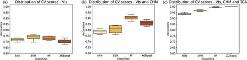
The CV score distribution shows that adding TCA as a feature helped improve classifier precision, as the distribution of CV scores became lower, especially in the XGBoost classifier (Figure 8c). This low variability indicates the classifier’s stability, with no overfitting, regardless of the CV k-fold used. The SVM classifier also had lower variability with the addition of TCA. The high precision and stability of the classifiers, especially RF and XGBoost, suggest that the combination of VIs, spectral bands, CHM, and TCA as features provides a robust approach for almond tree classification.

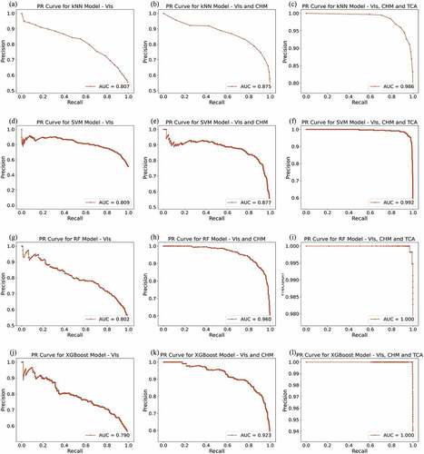
In Figure 9, plots show the precision versus the recall (= TPR) for several thresholds. The optimal results are associated with high PR AUC values. The best performance in PR AUC, using VIs and spectral bands (GREEN, GRVI, GN, REN, ClRE) was achieved in SVM classifier with an AUC of 0.81. The XGBoost classifier obtained a slightly lower performance with an AUC of 0.79. Considering the results using VIs, spectral bands and CHM, RF, and XGBoost classifiers performed better with AUCs of 0.96 and 0.92, respectively. On the other hand, the worst performance was obtained by kNN classifier (AUC = 0.88). When VIs, spectral bands, CHM, and TCA features were applied, the results obtained were very similar with an overall improvement in performance, with RF and XGBoost having the best AUCs (1.00).

Figure 9. Precision–recall curve, for each classifier (K-nearest neighbour (kNN), support vector machine (SVM), random forest (RF) and XGBoost): (a,d, g, j) using VI and spectral bands, (b, e, h, k) using VI, spectral bands and canopy height model (CHM) and (c, f, i, l) using VI, spectral bands, CHM and tree crown area (TCA).

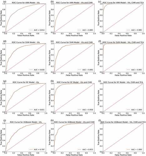
The receiver operating characteristic (ROC) curve plots the TPR versus the FPR for several thresholds (Figure 10). The lower the threshold, the greater the TPR, but also the FPR. The closer a classifier’s ROC curve is to the upper left corner, the better its performance. Using VIs and spectral bands (GREEN, GRVI, GN, REN, ClRE), SVM classifier obtained the best ROC AUC performance with an AUC of 0.83. With an AUC of 0.80, the XGBoost classifier had a slightly lower performance. The RF and XGBoost classifiers performed better using VIs, spectral bands, and CHM (AUC = 0.96 and 0.92, respectively). The classifier with the poorest performance was the kNN classifier (AUC = 0.89). When VIs, spectral bands, CHM, and TCA features were implemented, the overall performance improved, with RF and XGBoost having the best AUCs (1.00).

Figure 10. Receiver operating characteristics curve (ROC) for each classifier (K-nearest neighbour (kNN), support vector machine (SVM), random forest (RF) and XGBoost): (a,d, g, j) using VI and spectral bands, (b, e, h, k) using VI, spectral bands, and canopy height model (CHM) and (c, f, i, l) using VI, spectral bands, CHM and tree crown area (TCA).

4. Discussion

In this study, the aim was to prove the effectiveness of various features in the classification of almond cultivars. Seven features were selected including VIs, spectral bands, and structural parameters, and implemented in four ML classifiers. The TCA feature was found to be the most significant predictor of the target variable and showed that Francolí cultivar had higher values compared to Lauranne cultivar, indicating differences in vigour. The ML classifiers RF and XGBoost performed better than kNN and SVM classifiers.

Considering studies that applied ML classifiers, Borges et al. (Borges et al. 2021) classified the intertidal reef using RGB and multispectral imagery obtained by UAV. The researchers classified sand; rock, barnacles, limpets; mussels, rock; and algae mixed using four machine learning classifiers: SVM, artificial neural networks (ANN), NB, and RF. According to the obtained results, the SVM classifier performed the best overall accuracy (67%), whereas the remaining classifiers performed between 61%, 64% and 65%, respectively, for the RF, ANN, and NB. In a study by Ahmed et al. (2017), authors also used RGB and multispectral imagery, acquired by UAV, to identify five classes (forest, shrub, herbaceous, bare soil, and built-up). The RF classifier was applied and obtained an OA of 95%, using the multispectral data. Nevertheless, when consumer-grade RGB sensors with lower spectrum capabilities were employed, classification accuracy was reduced by 10% to 15%. Regarding previous studies related to tree cultivar classification, Gomes et al. (2020) applied the leaf reflectance information in olive varieties classification. The authors analysed the performance of six ML classifiers: Classification and Regression Trees (CART), Stochastic Gradient Boosting Machine (GBM), XGBoost, RF, kNN, and SVM. They considered 2150 features, which constituted a severe constraint to the classifier training and testing process. Therefore, feature extraction and dimensional reduction approaches were implemented to optimize the data processing. Regarding the results, SVM classifier with dimensional reduction performed by Class-Paired LDA (OA = 82%) was the best performer. Indeed, when the number of features is large and exceeds the number of samples, SVM classifier performs better. Avola et al. (2019) also applied VIs in the classification process and used univariate (ANOVA) and multivariate (principal component analysis – PCA and linear discriminant analysis – LDA) approaches to identify olive cultivars using 14 VIs. They attained a classification accuracy of 90.9% using LDA for scions but failed to classify more than 68.2% of rootstocks.

Previous studies exhibited high values of OA. However, additional metrics must be considered in the evaluation of classifiers suitability. In case of having an unbalanced distribution of samples in classes, classifiers can be affected by prevalent classes contributing to achieving higher OA. Nevertheless, this can be ineffective classifiers, as other metrics such as recall, and f1score are required to evaluate the number of right predictions in each class. According to the results obtained, in this study, for kNN, SVM, RF and XGBoost classifiers, recall, and F1-score present similar values when compared to precision and OA, which indicates that they are suitable classifiers with a regular performance in each class.

Regarding the features selected for the classification process. The best results were achieved using VIs and spectral bands (GREEN, GRVI, GN, REN, ClRE) with structural parameters (CHM and TCA), where overall accuracy values were close to 1.00. Due to the use of data with varying levels of water stress (data from 2021 June and 2022 July), the classification of almond cultivars is challenged by the results obtained when only considering the VIs and spectral bands. In many studies, the impact of water stress on the physiological and morphological characteristics of trees is addressed which can compromise the cultivar classification. In a study by Laskari et al., the authors discussed the effects of water stress on the morphological and physiological characteristics of maize plants, as well as the environmental cost of water stress. They found that water stress caused a reduction in plant height, leaf area, and chlorophyll content, as well as an increase in stomatal conductance and proline content (Laskari et al. 2022).

Despite the complexity, both in terms of exigency and difficulty, associated with tree cultivar classification, the use of VIs and spectral bands, when combined with structural parameters, show promising results. The detected variation in the features of each cultivar and the metrics derived from the application of ML classifiers demonstrated the viability of this process. Furthermore, this study also demonstrates that using machine learning to classify almond cultivars can automate the process of cultivar identification and, consequently, improve crop management by adjusting specific fertilization and irrigation regimes tailored to each cultivar’s needs, identifying, and isolating diseased plants, optimizing harvest schedule, improving quality control, predict yields, and support decision-making.

In future studies, it should be assessed whether the effects on tree development and pruning activities influence the classification accuracy. This will support the decision of whether this method can be applied to a single orchard or if it is adaptable to several orchards. Therefore, it is important to continue testing the classifiers under different conditions to ensure that it generalizes well and can be applied to a wide range of real-world scenarios.

5. Conclusions

In this study, a precision agriculture approach is employed for almond cultivar classification based on multispectral UAV data and ML. Despite its importance, studies applying VIs, spectral bands, and structural parameters for image classification, specifically for tree cultivar classification, are scarce. Cultivar classification is, indeed, a complex task that is dependent on data quality and feature selection, which should be carefully chosen based on its variability and relevance for classifier application. The cultivars addressed in this study, Francolí and Lauranne, present several differences in their characteristics, namely in crown structure, production levels, and vigour, which contributed to enhancing the classification process.

The obtained results demonstrate the usefulness of ML classifiers for tree cultivars classification. The four applied classifiers produced significant results, with particular attention on the RF (OA = 99%), XGBoost (OA = 99%), and SVM (OA = 96%) classifiers, which achieved the best results. The proposed methodology can be applied on a larger scale to other almond crops and distinct cultivars but can also be easily adapted to classify between different crop species for better inventory.

Acknowledgements

Financial support was provided by national funds through FCT – Portuguese Foundation for Science and Technology (UI/BD/150727/2020), under the Doctoral Programme “Agricultural Production Chains – from fork to farm” (PD/00122/2012) and from the European Social Funds and the Regional Operational Programme Norte 2020. This study was also supported by CITAB research unit (UIDB/04033/2020). We also acknowledge the CoaClimateRisk project (COA/CAC/0030/2019).

Disclosure statement

No potential conflict of interest was reported by the author(s).

Additional information

Funding

The work was supported by the Fundacao para a Ciência e a Tecnologia [PD/00122/2012, UI/BD/150727/2020, UIDB/04033/2020].

References

- Ahmed, O. S., A. Shemrock, D. Chabot, C. Dillon, G. Williams, R. Wasson, and S. E. Franklin. 2017. “Hierarchical Land Cover and Vegetation Classification Using Multispectral Data Acquired from an Unmanned Aerial Vehicle.” International Journal of Remote Sensing 38 (8–10): 8–10–20522037–2052. Taylor & Francis. doi:10.1080/01431161.2017.1294781.
- Antje, K., and C. S. Signorino. 2018. “Using Support Vector Machines for Survey Research.” Survey Practice 11 (1): 1–14. doi:10.29115/SP-2018-0001.
- Avola, G., S. Filippo Di Gennaro, C. Cantini, E. Riggi, F. Muratore, C. Tornambè, and A. Matese. 2019. “Remotely Sensed Vegetation Indices to Discriminate Field-Grown Olive Cultivars.” Remote Sensing 11 (10): 10–1242. Multidisciplinary Digital Publishing Institute. doi:10.3390/rs11101242.
- Ayan, E., and H. Murat Ünver. 2018. “Data Augmentation Importance for Classification of Skin Lesions via Deep Learning.” 2018 Electric Electronics, Computer Science, Biomedical Engineerings’ Meeting (EBBT), 1–4. doi:10.1109/EBBT.2018.8391469.
- Baf, S., E. Im, and M. Bol. 2013. “Application of K-Nearest Neighbor (KNN) Approach for Predicting Economic Events: Theoretical Background.“ Int. Journal of Engineering Research and Applications 3: 605–610.
- Beek, V., L. T. Jonathan, B. Somers, and P. Coppin. 2013. “Stem Water Potential Monitoring in Pear Orchards through WorldView-2 Multispectral Imagery.” In Remote Sensing Vol. 5 (12), 6647–6666. Multidisciplinary Digital Publishing Institute. doi:10.3390/rs5126647.
- Belgiu, M., and L. Drăguţ. 2016. “Random Forest in Remote Sensing: A Review of Applications and Future Directions.” Isprs Journal of Photogrammetry and Remote Sensing 114 (April): 24–31. doi:10.1016/j.isprsjprs.2016.01.011.
- Borges, D., L. Padua, I. Costa Azevedo, J. Silva, J. J. Sousa, I. Sousa–Pinto, and J. Alberto Gonçalves. 2021. “Classification of an Intertidal Reef by Machine Learning Techniques Using UAV Based RGB and Multispectral Imagery.” 2021 IEEE International Geoscience and Remote Sensing Symposium IGARSS, 64–67. doi:10.1109/IGARSS47720.2021.9554221.
- Chandrashekar, G., and F. Sahin. 2014. “A Survey on Feature Selection Methods.” Computers & Electrical Engineering, 40th-Year Commemorative Issue 40 (1): 16–28. doi:10.1016/j.compeleceng.2013.11.024.
- Chenari, A., Y. Erfanifard, M. Dehghani, and H. R. Pourghasemi. 2017. “Woodland Mapping at Single-Tree Levels Using Object-Oriented Classification of Unmanned Aerial Vehicle (Uav) Images.” The International Archives of the Photogrammetry, Remote Sensing and Spatial Information Sciences, no. September: 43–49. doi:10.5194/isprs-archives-XLII-4-W4-43-2017.
- Chen, Z., F. Jiang, Y. Cheng, G. Xin, W. Liu, and J. Peng. 2018. “XGBoost Classifier for DDoS Attack Detection and Analysis in SDN-Based Cloud.” 2018 IEEE International Conference on Big Data and Smart Computing (BigComp), 251–256. doi:10.1109/BigComp.2018.00044.
- Cordeiro, V., C. Alves, J. Vieira, and M. R. Barroso. 2005. “Evaluation of Almond Cultivar Adaptation in Trás-Os-Montes Region (Portugal).“ XIII GREMPA Meeting on Almonds and Pistachios, Zaragoza, 2005, 63: 5.
- Csillik, O., J. Cherbini, R. Johnson, A. Lyons, and M. Kelly. 2018. “Identification of Citrus Trees from Unmanned Aerial Vehicle Imagery Using Convolutional Neural Networks.” Drones 2 (4): 39. Multidisciplinary Digital Publishing Institute. doi:10.3390/drones2040039.
- Dainelli, R., P. Toscano, S. Filippo Di Gennaro, and A. Matese. 2021. “Recent Advances in Unmanned Aerial Vehicles Forest Remote Sensing—a Systematic Review. Part II: Research Applications.” Forests 12 (4): 4–397. Multidisciplinary Digital Publishing Institute. doi:10.3390/f12040397.
- Daponte, P., L. De Vito, L. Glielmo, L. Iannelli, D. Liuzza, F. Picariello, and G. Silano. 2019. “A Review on the Use of Drones for Precision Agriculture.” IOP Conference Series: Earth and Environmental Science, IOP Publishing, May 012022–275. doi:10.1088/1755-1315/275/1/012022.
- Davis, J., and M. Goadrich. 2006. “The Relationship Between Precision-Recall and ROC Curves.”Proceedings of the 23rd International Conference on Machine Learning - ICML, Pittsburgh, Pennsylvania: ACM Press 06, 233–240. doi:10.1145/1143844.1143874.
- de Herralde, F., R. Savé, C. Biel, I. Batlle, and F. J. Vargas. 2001. “Differences in Drought Tolerance in Two Almond Cultivars: ‘Lauranne’ and ‘Masbovera,’.“ XI GREMPA Seminar on Pistachios and Almonds, Zaragoza, 2001, 7: 149–154.
- Egea, J., E. Ortega, P. Martı́nez-Gómez, and F. Dicenta. 2003. “Chilling and Heat Requirements of Almond Cultivars for Flowering.” Environmental and Experimental Botany 50 (1): 79–85. doi:10.1016/S0098-8472(03)00002-9.
- Eli-Chukwu, N. C. 2019. “Applications of Artificial Intelligence in Agriculture: A Review.” Engineering, Technology & Applied Science Research 9 (4): 4377–4383. doi:10.48084/etasr.2756.
- Fassnacht, F. E., H. Latifi, K. Stereńczak, A. Modzelewska, M. Lefsky, L. T. Waser, C. Straub, and A. Ghosh. 2016. “Review of Studies on Tree Species Classification from Remotely Sensed Data.” Remote Sensing of Environment 186 (December): 64–87. doi:10.1016/j.rse.2016.08.013.
- Fiorucci, F., F. Ardizzone, A. Cesare Mondini, A. Viero, and F. Guzzetti. 2018. “Visual Interpretation of Stereoscopic NDVI Satellite Images to Map Rainfall-Induced Landslides.” Landslides 1 (16): 165–174. doi:10.1007/s10346-018-1069-y.
- Ghamisi, P., B. Rasti, N. Yokoya, Q. Wang, B. Hofle, L. Bruzzone, F. Bovolo, et al. 2019. “Multisource and Multitemporal Data Fusion in Remote Sensing: A Comprehensive Review of the State of the Art.” IEEE Geoscience and Remote Sensing Magazine 7 (1): 6–39. doi:10.1109/MGRS.2018.2890023.
- Gitelson, A. A., Y. J. Kaufman, and M. N. Merzlyak. 1996. “Use of a Green Channel in Remote Sensing of Global Vegetation from EOS-MODIS.” Remote Sensing of Environment 58 (3): 289–298. doi:10.1016/S0034-4257(96)00072-7.
- Gomes, L., T. Nobre, A. Sousa, F. Rei, and N. Guiomar. 2020. “Hyperspectral Reflectance as a Basis to Discriminate Olive Varieties—a Tool for Sustainable Crop Management.” Sustainability 12 (7): 3059. doi:10.3390/su12073059.
- Grandini, M., E. Bagli, and G. Visani. August 2020. “Metrics for Multi-Class Classification: An Overview.” ArXiv: 2008 05756 [Cs, Stat]. http://arxiv.org/abs/2008.05756.
- Haara, A., and M. Haarala. 2002. “Tree Species Classification Using Semi-Automatic Delineation of Trees on Aerial Images.” Scandinavian Journal of Forest Research 17 (6): 556–565. Taylor & Francis. doi:10.1080/02827580260417215.
- Horning, N. 2010. “Random Forests: An Algorithm for Image Classification and Generation of Continuous Fields Data Sets.“ International Conference on Geoinformatics for Spatial Infrastructure Development in Earth and Allied Sciences, Japan, 2010, 911: 6.
- Huete, A. R. 1988. “A Soil-Adjusted Vegetation Index (SAVI).” Remote Sensing of Environment 25 (3): 295–309. doi:10.1016/0034-4257(88)90106-X.
- Huete, A., K. Didan, T. Miura, E. P. Rodriguez, X. Gao, and L. G. Ferreira. 2002. “Overview of the Radiometric and Biophysical Performance of the MODIS Vegetation Indices.” Remote Sensing of Environment 83 (1): 195–213. doi:10.1016/S0034-4257(02)00096-2.
- Inoue, H. 2018. “Data Augmentation by Pairing Samples for Images Classification.” ArXiv:1801.02929 [Cs, Stat], April. http://arxiv.org/abs/1801.02929.
- Jafarbiglu, H., and A. Pourreza. 2022. “A Comprehensive Review of Remote Sensing Platforms, Sensors, and Applications in Nut Crops.” Computers and Electronics in Agriculture 197: 23. doi:10.1016/j.compag.2022.106844.
- Jha, K., A. Doshi, P. Patel, and M. Shah. 2019. “A Comprehensive Review on Automation in Agriculture Using Artificial Intelligence.” Artificial Intelligence in Agriculture 2 (June): 1–12. doi:10.1016/j.aiia.2019.05.004.
- Kok, Z. H., A. Rashid Mohamed Shariff, M. S. M. Alfatni, and S. Khairunniza-Bejo. 2021. “Support Vector Machine.” Computers and Electronics in Agriculture 191 (December): 106546. doi:10.1016/j.compag.2021.106546.
- Laskari, M., G. Menexes, I. Kalfas, I. Gatzolis, and C. Dordas. 2022. “Water Stress Effects on the Morphological, Physiological Characteristics of Maize (Zea Mays L.), and on Environmental Cost.” Agronomy 12 (10): 2386. doi:10.3390/agronomy12102386.
- Lisein, J., A. Michez, H. Claessens, and P. Lejeune. 2015. “Discrimination of Deciduous Tree Species from Time Series of Unmanned Aerial System Imagery.” In PLOS ONE. edited by M. Cristani, Vol. 10, e0141006. 11. doi: 10.1371/journal.pone.0141006.
- Loussaief, S., and A. Abdelkrim. 2016. “Machine Learning Framework for Image Classification.”2016 7th International Conference on Sciences of Electronics, Technologies of Information and Telecommunications, (SETIT), 58–61. doi:10.1109/SETIT.2016.7939841.
- Mateo-Aroca, A., G. García-Mateos, A. Ruiz-Canales, J. María Molina-García-Pardo, and J. Miguel Molina-Martínez. 2019. “Remote Image Capture System to Improve Aerial Supervision for Precision Irrigation in Agriculture.” Water 11 (2): 255. Multidisciplinary Digital Publishing Institute. doi:10.3390/w11020255.
- Mavridou, E., E. Vrochidou, G. A. Papakostas, T. Pachidis, and V. G. Kaburlasos. 2019. “Machine Vision Systems in Precision Agriculture for Crop Farming.” Journal of Imaging 5 (12): 89. doi:10.3390/jimaging5120089.
- Miarnau, X., S. Alegre, and F. Vargas. 2010. “Productive Potential of Six Almond Cultivars Under Regulated Deficit Irrigation.“ XIV GREMPA Meeting on Pistachios and Almonds, Zaragoza, 2010, 94: 6.
- Michel, J., D. Youssefi, and M. Grizonnet. 2014. “Stable Mean-Shift Algorithm and Its Application to the Segmentation of Arbitrarily Large Remote Sensing Images.” IEEE Transactions on Geoscience and Remote Sensing 53 (2): 952–964. doi:10.1109/TGRS.2014.2330857.
- Noble, W. S. 2006. “What is a Support Vector Machine?” Nature Biotechnology 24 (12): 1565–1567. doi:10.1038/nbt1206-1565.
- Pádua, L., T. Adão, J. Hruška, J. J. Sousa, E. Peres, R. Morais, and A. Sousa. 2017. “Very High Resolution Aerial Data to Support Multi-Temporal Precision Agriculture Information Management.” Procedia Computer Science, CENTERIS 2017 - International Conference on ENTERprise Information Systems/ProjMAN 2017 - International Conference on Project MANagement/HCist 2017 - International Conference on Health and Social Care Information Systems and Technologies, CENTERIS/ProjMAN/HCist 2017, 121 (January): 407–414. doi:10.1016/j.procs.2017.11.055.
- Pádua, L., P. Marques, L. Martins, A. Sousa, E. Peres, and J. J. Sousa. 2020. “Monitoring of Chestnut Trees Using Machine Learning Techniques Applied to UAV-Based Multispectral Data.” Remote Sensing 12 (18): 3032. doi:10.3390/rs12183032.
- Pathak, T. B., M. L. Maskey, and J. P. Rijal. 2021. “Impact of Climate Change on Navel Orangeworm, a Major Pest of Tree Nuts in California.” The Science of the Total Environment 755 (February): 142657. doi:10.1016/j.scitotenv.2020.142657.
- Pedro, M., L. Pádua, T. Adão, J. Hruška, E. Peres, A. Sousa, and J. J. Sousa. 2019. “UAV-Based Automatic Detection and Monitoring of Chestnut Trees.” Remote Sensing 11 (7): 855. doi:10.3390/rs11070855.
- Pinter, P. J., Jr., J. L. Hatfield, J. S. Schepers, E. M. Barnes, M. Susan Moran, C. S. T. Daughtry, and D. R. Upchurch. 2003. “Remote Sensing for Crop Management.” Photogrammetric Engineering & Remote Sensing 69 (6): 647–664. doi:10.14358/PERS.69.6.647.
- Preethi, C., N. C. Brintha, and C. K. Yogesh 2021. “An Comprehensive Survey on Applications of Precision Agriculture in the Context of Weed Classification, Leave Disease Detection, Yield Prediction and UAV Image Analysis.” In Advances in Parallel Computing, edited by D. J. Hemanth, M. Elhosney, T. N. Nguyen, and S. Lakshmanan. “An Comprehensive Survey on Applications of Precision Agriculture in the Context of Weed Classification, Leave Disease Detection, Yield Prediction and UAV Image Analysis.” in Advances in Parallel Computing. edited by. IOS Press. doi: 10.3233/APC210152.
- Probst, P., B. Bischl, and A.L. Boulesteix. 2018. “Tunability: Importance of Hyperparameters of Machine Learning Algorithms.” arXiv. http://arxiv.org/abs/1802.09596.
- Reid, A., F. Ramos, and S. Sukkarieh. 2011. “Multi-Class Classification of Vegetation in Natural Environments Using an Unmanned Aerial System.”2011 IEEE International Conference on Robotics and Automation, Shanghai, China: IEEE 2953–2959. doi:10.1109/ICRA.2011.5980061.
- Ren, S., X. Chen, and A. Shuai. 2017. “Assessing Plant Senescence Reflectance Index-Retrieved Vegetation Phenology and Its Spatiotemporal Response to Climate Change in the Inner Mongolian Grassland.” International Journal of Biometeorology 61 (4): 601–612. doi:10.1007/s00484-016-1236-6.
- Rodrigues, P., A. Venâncio, and N. Lima. 2012. “Mycobiota and Mycotoxins of Almonds and Chestnuts with Special Reference to Aflatoxins.” Food Research International 48 (1): 76–90. doi:10.1016/j.foodres.2012.02.007.
- Rouse, J. W., Jr., R. H. Haas, J. A. Schell, and D. W. Deering. 1974. “Monitoring Vegetation Systems in the Great Plains with Erts.” NASA Special Publication 351 (January): 309.
- Saito, T., M. Rehmsmeier, and G. Brock. 2015. “The Precision-Recall Plot is More Informative Than the ROC Plot When Evaluating Binary Classifiers on Imbalanced Datasets.” Plos One 10 (3): e0118432. doi:10.1371/journal.pone.0118432.
- Soares, C., P. Rodrigues, S. W. Peterson, N. Lima, and A. Venâncio. 2012. “Three New Species of Aspergillus Section Flavi Isolated from Almonds and Maize in Portugal.” Mycologia 104 (3): 682–697. Taylor & Francis. doi:10.3852/11-088.
- Sumner, D. A., W. A. Matthews, J. Medellín-Azuara, and A. Bradley University of California. 2016. The Economic Impacts of the California Almond Industry. California: Almond Board of California.
- Taha, B., and A. Shoufan. 2019. “Machine Learning-Based Drone Detection and Classification: State-Of-The-Art in Research.” IEEE Access 7: 138669–138682. doi:10.1109/ACCESS.2019.2942944.
- Tucker, C. J. 1979. “Red and Photographic Infrared Linear Combinations for Monitoring Vegetation.” Remote Sensing of Environment 8 (2): 127–150. doi:10.1016/0034-4257(79)90013-0.
- Yaping, X., V. Shrestha, C. Piasecki, B. Wolfe, L. Hamilton, R. J. Millwood, M. Mazarei, and C. Neal Stewart. 2021. “Sustainability Trait Modeling of Field-Grown Switchgrass (Panicum Virgatum) Using UAV-Based Imagery.” In Plants Vol. 10 (12), 2726. Multidisciplinary Digital Publishing Institute. doi:10.3390/plants10122726.
- Zhou, H., X. Wang, and G. Schaefer. 2011. “Mean Shift and Its Application in Image Segmentation.” In Innovations in Intelligent Image Analysis, edited by H. Kwaśnicka and L. C. Jain, 291–312, Vol. 339. Studies in Computational Intelligence. Berlin, HeidelbergBerlin Heidelberg: Springer. doi:10.1007/978-3-642-17934-1_13.