On the temporal mismatch between in-situ and satellite-derived spring phenology of European beech forests

ABSTRACT

Forest phenology plays a key role in the global terrestrial ecosystem influencing a range of ecosystem processes such as the annual carbon uptake period, and many food webs and changes in their timing and progression. The timing of the start of the phenology season has been successfully determined at a range of scales, from the individual tree by in situ observations to landscape and continental scales by using remotely sensed vegetation indices (VIs). The spatial resolution of satellites is much coarser than traditional methods, creating a gap between space-borne and actual field observations, which brings limitations to phenological research at the ecosystem level. Several unconsidered methodological and observational-related limitations may lead to misinterpretation of the timing of the satellite-derived signals. The aim of this study is therefore to clarify the meaning of a set of spring phenology metrics derived from Moderate Resolution Imaging Spectroradiometer (MODIS) Enhanced Vegetation Index (EVI) time series in beech forests distributed across Europe with respect to PEP725 in situ observations, from 2003 to 2020. To this aim, we (i) tested the differences between remotely sensed and in situ start-of-season (SOS) metrics and (ii) quantified the influence of latitude, elevation, temperature, and precipitation on such differences. Results demonstrated that there is a clear temporal gradient among the different SOS metrics, all of them occurring prior to the in situ observations. Furthermore, latitude and temperatures proved to be the main factors guiding the differences between remotely sensed and in situ SOS metrics. Evidence from this study may help in recognizing the actual meaning of what we see by means of remotely sensed phenology metrics. In this perspective, field observations are crucial in understanding phenology events and provide a reference base. Satellite data, on the other hand, complement field observations by filling in gaps in spatial and temporal coverage, thus enhancing the overall understanding.

KEYWORDS:

• Beech forest
• bioclimatic variables
• MODIS EVI
• PEP725
• phenology
• remote sensing

1. Introduction

Forest communities play a key role in the global ecosystem dynamics and pivotal to this role is forest phenology which influences ecological processes at several scales. Forest phenology determines the different phases of the growing season which in turn affect, for example, the annual carbon uptake (Piao et al. 2007; Richardson et al. 2013; Keenan et al. 2014; Hufkens et al. 2016), as well as resource availability at all trophic levels (Both et al. 2009; Donnelly and Yu 2021).

The timing of the start and end of the phenology season has been successfully determined at a range of scales (Bórnez et al. 2020; Chianucci, Bajocco, and Ferrara 2021) from the individual tree, by in situ observation (Fu et al. 2015; Zheng et al. 2016), to landscape and continental scales, by satellite remote sensing (Henebry and de Beurs 2013; Liu et al. 2017).

Prior to recent technology advancements, the most common method of monitoring vegetation phenological dynamics was to manually record human observations at discrete intervals of individual plant or species life cycle events, such as bud break, flowering, or leaf senescence (Verhegghen, Bontemps, and Defourny 2014). Recently, continuous images from fixed digital cameras, e.g. the PhenoCam network or camera traps (Chianucci, Bajocco, and Ferrara 2021), have been used to provide ground-based vegetation phenological observations. However, significant limitations exist in monitoring phenology at the ground level, mainly due to the difficulty of (i) harmonizing data records over plant species and phenological events; (ii) using such data at global or regional scales due to the time and efforts consuming nature of field observations; (iii) integrating field data with observations of climatic variables which have a very coarse spatial resolution; and (iv) extending the phenological events identified from individual species to communities (Studer et al. 2007; White et al. 2009). Alternatively, remotely sensed phenology or land surface phenology (LSP) is defined as the seasonal pattern of variation of vegetation indices (i.e. greening, senescence, dormancy, etc.) in vegetated land surfaces observed from satellite remote sensing (De Beurs and Henebry 2005; Zeng et al. 2020). Satellite observations constitute a spatially aggregated signal from heterogeneous surface conditions that may not be representative of any single plant species response (pixel size from metres to km) (D’odorico et al. 2015), but rather of a single- or multi-species community. The spatial resolution of satellites is much coarser than traditional methods, creating a gap between remotely sensed and field observations, and therefore undermining the phenological research at the ecosystem level (Jorge et al. 2021).

As a consequence, as stated by Zhang et al. (2018), pixel-based remotely sensed phenology cannot precisely reflect in situ conditions of individual trees and shrubs, highlighting the importance of scale of observation when comparing phenological metrics (Donnelly and Yu 2021). LSP metrics are typically associated with general intra-annual vegetation canopy changes detectable from spectral remote-sensing imagery. From the temporal profiles of vegetation indices (VIs), like the Normalized Difference Vegetation Index (NDVI) or the Enhanced Vegetation Index (EVI), several statistical techniques have been developed to extract phenological metrics in terms of green-up/start of season, peak of growing season, senescence/end of season, and length of the growing season (Reed et al. 1994; de Beurs and Henebry 2010). The derived phenological metrics are strictly dependent on the sensors, and their spatial and temporal resolution, adding variability and uncertainty in the estimation. The length of the time series (from 10 to 30 years), the high temporal frequency (from twice daily to 5 days), internal consistency, and continuous availability of the satellite measurements are therefore fundamental requirements when dealing with vegetation phenology (Restrepo-Coupe, Huete, and Davies 2015). Accordingly, one of the most used satellites for phenological studies is the Moderate Resolution Imaging Spectroradiometer (MODIS) that with a long-term archive (since 2000), a moderate spatial resolution (250 m), and a high temporal resolution (daily) represents a good trade-off (Bajocco et al. 2019).

Apart from the spatial mismatch, several observational-related mismatches may also lead to misinterpretation of the satellite-derived signals (Morton et al. 2014). For instance, changes in species composition within a pixel could determine a change in the temporal profile of the VI, due to the different phenological responses of the different plant species involved; this may lead to the signal change being misinterpreted as a phenological change when actually it is not (Helman 2018). Other limitations are related to the mixed signal from multi-canopy layers. In this case, changes may be real, but could correspond to changes in the earliest species in the pixel (Fu et al. 2014), which is not necessarily the most dominant plant species in that biome (Helman et al. 2015). Satellites may detect signal changes that depend on the understory layer in complex vertical vegetation systems, potentially affecting the timing of the extracted phenology metrics as well as the sign of the observed phenology change (Helman 2018).

While the alignment between in situ and satellite phenological observations and related accuracy have been largely quantified and tested (Sivasathivel Kandasamy and Fernandes 2015; Verger et al. 2016; Bórnez et al. 2020), the biophysical meaning of such temporal mismatch received far less attention. The objectives of this research are thus (i) to better understand the temporal discrepancy between a set of field- and satellite-based spring phenology indicators in European beech (Fagus sylvatica) forests, and (ii) to quantify the influence of the main biophysical factors (i.e. latitude, elevation, temperature, and precipitation) on such mismatch. Even though the impact of climate and geographical characteristics on observed phenology has been largely studied (e.g. (Bajocco et al. 2019; Ivits et al. 2012; Caparros-Santiago, Rodriguez-Galiano, and Dash 2021; Yuan et al. 2022)), to the best of our knowledge, the role of these variables on the relationship between remotely sensed and in situ phenology is still unexplored. Overall, this study is not focusing on the different accuracy of remotely sensed vs in situ observed phenology, but on the additional information that can be obtained from satellite-based phenological data and on the benefits of integrating both approaches.

2. Materials and methods

2.1. Phenological observations

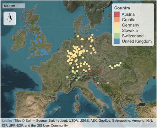
The ground-based phenological time-series was extracted from the Pan-European Phenology (PEP725; www.pep725.eu) database and used as reference data. PEP725 has complete records from 1990 to the present (Templ et al. 2018). The phenophases defined in PEP725 are based on BBCH (Biologische Bundesanstalt, Bundessortenamt and Chemical industry) codes (Meier et al. 2009). In this study, all the PEP725 stations with Fagus sylvatica as forest species were selected and data for the period 2003–2020 were downloaded, in accordance with the time frame of satellite observations (Figure 1). We used the phenophases corresponding to the first visible leaves (BBCH 11 and BBCH 13) as the reference for the timing of SOS, being the most common observed codes relevant to the SOS phenology. We discarded ground sites with less than four yearly measurements to obtain consistent data records over the time series.

Figure 1. Distribution of selected PEP725 stations by country across Europe.

The time series of satellite imagery used for estimating the phenological metrics were derived from the Moderate Resolution Imaging Spectroradiometer (MODIS) Terra and Aqua sensors, from 2003 to 2020, with spatial resolution of 250 m and temporal frequency of 8 days. We used the MOD13Q1 and MYD13Q1 maximum value composite (MVC) enhanced vegetation index (EVI) products. The MVC procedure allows to reduce noise from the available series for each pixel, since only the highest EVI value for a given period is retained as representative (Holben 1986). This technique, while keeping a regular temporal resolution, minimizes atmospheric and geometric effects in optical imagery. We used EVI in this study because, even if the normalized difference vegetation index (NDVI) is the most often used green index for studying vegetation, it tends to saturate over dense canopies, such as forested areas, losing sensitivity (Gitelson 2004). Instead, EVI was proposed as a modified NDVI, having a wider dynamic range and correction for atmospheric and soil background. As a result, EVI is more sensitive than NDVI in detecting forest seasonal changes, particularly over dense and large canopy backgrounds such as broadleaved forests (Huete et al. 2002).

We selected all the PEP725 stations with Fagus sylvatica as forest species and applied two filters to link MODIS data with PEP725 records while minimizing their spatial mismatch. To reduce the possibility of including non-forested/ambiguous sites in our study, a first filter was applied to consider only PEP725 records falling within large, forested areas (i.e. excluding small, heterogeneous, edge- or non-forested areas). PEP725 stations were thus intersected with the 2018 European Corine Land Cover (CLC) map (1:100,000, minimum mapping unit of 25 ha, and minimum polygon width of 100 m), and only PEP725 records belonging to the broad-leaved forests Corine Land Cover category (311) were kept for further analysis. Secondarily, PEP725 stations with at least one EVI temporal band value lower than or equal to zero were removed to reduce the probability of considering zones with, for example, water or bare soil, as well as to avoid areas completely or partly covered by snow and to consider only densely forested pixels. As a result, we got a total of 140 PEP725 stations comprising a total of 950 observations.

2.2. Biophysical data

The elevation (ELEV; m) was extracted from the ASTER Global Digital Elevation Model (GDEM) V2 product; it has a 30 m spatial resolution and is freely available at https://asterweb.jpl.nasa.gov/gdem.asp. The latitude in UTM projection (LAT; m) was extracted from the geographical coordinates of the PEP725 stations.

The bioclimatic variables were derived from the WorldClim V2 dataset (http://www.worldclim.org/bioclim) which is a set of 1970–2000 global climate layers (monthly gridded temperature and precipitation data) with a spatial resolution of 1 km. The selected bioclimatic variables indicate Mean Temperature (T_mean; °C × 10) and Annual Precipitation (P_tot; mm) (Hijmans et al. 2005; Fick and Hijmans 2017).

In this work, we used climate data rather than meteorological data because we are interested on the climate traits and conditions than on the local weather variations. Furthermore, the temporal discrepancy between the bioclimatic and MODIS data may be overcome because any patterns of change in the mean values may be trivial given the inertia of vegetation, as well as the main regional climate drivers (i.e. latitude and elevation) and the coarse expectations of the analysis (Bajocco et al. 2019).

2.3. Phenometrics extraction

Firstly, a running mean filter with a 5 × 5 sliding window was applied for smoothing the EVI temporal profiles. Then, using the phenofit R package (Kong et al. 2022), we performed the fitting of the EVI temporal profile and the SOS metrics extraction. To reconstruct daily EVI time series, we used the double logistics function method proposed by Elmore et al. (2012) as curve fitting method (Elmore et al. 2012). SOS phenological metrics were extracted from the daily time series by means of different methods available in the phenofit R package: (i) Threshold method, (ii) Derivative method, (iii) Gu method and (iii) Zhang method (Table 1).

Table 1. Phenophases description with related extraction methods. BBCH corresponds to field observations, while the remaining metrics are satellite-based.

Metrics	Description
BBCH	Phenological phases of PEP725 relevant to first leaves unfolded (BBCH 11) and more leaves unfolded (BBCH 13).
DER	Derivative method deriving the DOY when the first derivative reaches the maximum value.
TRS2	Threshold method deriving the DOY when the curve reaches the 20% of the seasonal amplitude.
TRS5	Threshold method deriving the DOY when the curve reaches the 50% of the seasonal amplitude.
GU	Gu method deriving the DOY of the upturn date (UD), based on a combination of local maxima in the first derivative.
ZHANG	Zhang method deriving the DOY of the onset of photosynthetic activity (green-up), calculated using minimum and maximum values in the rate of change in curvature.

In the threshold method, SOS is defined as the day of the year (DOY) when a vegetation variable exceeds a given threshold, i.e. the 20th and 50th percentiles of the annual amplitude for SOS (TRS2 and TRS5). In the derivative method (DER), SOS is defined as the DOY of the maximum in the first derivative (Tateishi and Ebata 2004). In the Gu method (GU), the first derivative maximum was used to define the line tangent to the curve and thus their intersection with the baseline defining the SOS upturn phenophase (Gu et al. 2009). In the Zhang method (ZHANG), the SOS green-up date was computed using the maximum value in the rate of change in curvature (Zhang et al. 2003).

2.4. Statistical analysis

To assess the differences between remotely sensed and in situ SOS, each metric has been compared with the BBCH start of season. The Bland-Altman plot was used to assess the agreement between BBCH and EVI-based SOS measurement techniques. It displays the differences between two techniques against their average. The plot helps to identify the mean difference between the two methods and any systematic bias or random variability. Normality was also checked performing the Shapiro–Wilk’s W test, which revealed that the data was not normally distributed. As a result, to explore the amount of the difference between the SOS dates of the five remotely sensed metrics and the BBCH, we computed the paired-sample Wilcoxon test, which is a non-parametric statistical method used to compare matched samples.

Then, we performed a Redundancy Analysis (RDA; (Rao 1964)) to quantify the role of the selected biophysical factors in explaining the differences between remotely sensed (i.e. DER, TRS5, TRS2, GU and ZHANG) and field-observed (i.e. BBCH) SOS dates (i.e. ΔDER, ΔTRS5, ΔTRS2, ΔGU and ΔZHANG). The method of RDA was developed by Rao (1964) and introduced to ecological data analysis by ter Braak and Prentice (1988). It is an asymmetric canonical ordination technique that measures redundancy (sensu Gittins 1979). That is, the proportion of the total variance of one set of response variables explained by a canonical variate from another set of explanatory variables. RDA can be seen as a constrained Principal Component Analysis (ter Braak and Prentice 1988): the ordination axes (F1 and F2) are linear combinations of the response variables, but they are also constrained to be a linear function of the predictor variables (Legendre and Legendre 1998). Accordingly, the ordination of the dependent variables is forced to be explained by the configuration of the independent variables such that the RDA axes represent the percentage of the variance of the response variables explained by the predictors (van den Brink and ter Braak 1999). In the RDA, the angles between vectors representing response variables and those representing explanatory variables reflect the strength of their (linear) correlation, while the vector direction indicates the positive or negative dependency (Legendre and Legendre 1998).

In our case, the biophysical variables served as predictors, whereas the temporal differences between the SOS dates of the five remotely sensed metrics and the BBCH served as response variables.

3. Results

3.1. Differences between remotely sensed and in situ start of season

The distribution of SOS dates of all the different metrics reveals a clear temporal gradient (Figure 2), ranging from ZHANG (mean DOY = 71.52), GU (mean DOY = 75.93), TRS2 (mean DOY = 83.28), TRS5 (mean DOY = 104.89), DER (mean DOY = 107.99) to BBCH (mean DOY = 111), with ZHANG, GU and TRS2 having the highest dispersion (Table 2). In detail, over time and for each of the 140 PEP725 stations, the BBCH metric tends to occur after the satellite metrics: in ZHANG, GU, and TRS2 almost 100% of remote observations occurred before BBCH, whereas in DER and TRS5 around 70% occurred before, ranging from 1 to 24 days earlier (data not shown here). Figure 3 shows an example of an EVI profile, representing the modelled fitting curve and the remotely sensed SOS phenology metrics together with the BBCH phenophase. This evidence suggested a separation of satellite metrics into two groups: those describing the early portion (TRS2, GU, and ZHANG) and those describing the late portion (TRS5 and DER) of the spring part of the growing season.

Figure 2. Temporal distribution of the SOS value densities for BBCH and the five phenological metrics detected from EVI time series (2003–2020). DOY, day of year.

Figure 3. Example of spring EVI profile (Germany: 48.7 longitude, 10.2 latitude, PEP725 Station: 2916, Year: 2008), showing the Elmore modelled curve (blue curve) and EVI-based phenology metrics (black dots) together with the PEP725 value (red dot). In the inset is depicted the corresponding annual EVI profile. DOY, day of year.

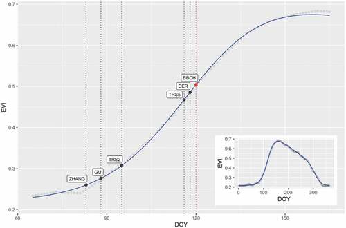
Table 2. Start of season summary statistics (DOY) for in situ and remotely sensed observations.

Statistics	BBCH	ZHANG	GU	TRS2	TRS5	DER
Mean	111.34	71.43	75.82	83.19	104.85	107.98
Std Dev	8.35	13.69	13.25	12.22	10.98	11.06
Std Err	0.27	0.43	0.42	0.38	0.35	0.35
Median	113.00	72.00	77.00	84.00	105.00	108.00
Range	63.00	97.00	97.00	88.00	88.00	89.00

The Bland–Altman plot in Figure 4 shows the difference of each SOS remotely sensed metric with BBCH, while results of the paired-sample Wilcoxon test are listed in Table 3. The paired-sample Wilcoxon test further confirmed the statistical significance of the temporal gradient across the SOS values, revealing that all remotely sensed SOS metrics tended to occur prior to the in situ observations, and that the metrics close to the BBCH values were TRS5 and DER. In detail, ZHANG meanly occurs 40 days before BBCH, GU about 36 days, TRS2 28 days, TRS5 about 7 days and DER about 4 days before BBCH. The metrics with the larger time-lag were those indicating a phenophase in the initial portion of the EVI curve, between the first abrupt increase and the 20% of the seasonal amplitude. On the contrary, the derivative metrics and the 50% of the seasonal amplitude resulted as the most in line with the ground-observed SOS, demonstrating a good correspondence between satellite and field observations, despite the inherent spatial mismatch.

Figure 4. Bland–Altman plot showing for each pair BBCH-remotely sensed metric the average (x-axis) plotted against their difference (y-axis). The blue line indicates the mean difference, including a confidence region for the mean of the differences.

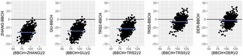
Table 3. Results of paired Wilcoxon test with reference to BBCH SOS values.

	ZHANG	GU	TRS2	TRS5	DER
Mean Difference	−40.17	−35.76	−28.42	−6.81	−3.71
Std Error	0.44	0.43	0.39	0.35	0.36
Upper 95%	−39.31	−34.93	−27.63	−6.12	−3.01
Lower 95%	−41.05	−36.62	−29.19	−7.51	−4.41
Wilcoxon signed rank test with continuity correction
V	395602	393814	394512	300492	256206
p-value	2.20E–16	2.20E–16	2.20E–16	2.20E–16	2.20E–16

3.2. Influence of the main biophysical factors

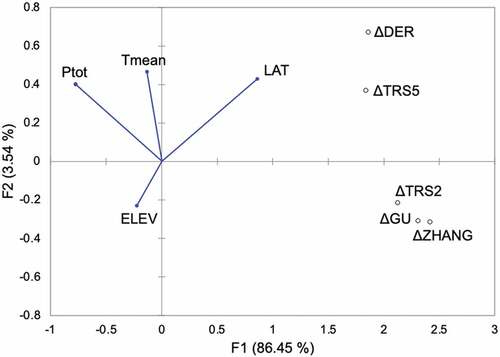
The RDA between biophysical variables (as predictors) and the differences between remotely sensed and in situ metrics (as response variables) explained almost 90% of variance. The biplot in Figure 5 shows that ΔDER and ΔTRS5 fall in the same quadrant with latitude and diametrically opposed to elevation, which means that large differences between DER and BBCH, and between TRS5 and BBCH are positively influences by latitude and negatively by elevation. Hence, at higher latitudes and lower elevations, the discrepancies between the later remotely sensed metrics and in situ observations increase. On the other hand, climate variables were the main predictors guiding the discrepancies between TRS2, GU, and ZHANG metrics, and BBCH, since ΔTRS2, ΔGU, and ΔZHANG fall in the opposite quadrant with respect to Ptot and Tmean. This means that, in case of drier conditions and lower mean temperatures, the earlier remotely sensed phenological metrics are further from the in situ observation.

Figure 5. Redundancy Analysis (RDA) biplot: distribution of the biophysical explanatory variables as vectors (blue arrows) and the phenological metrics difference (Δ) as response variables (black points). The first two RDA factors (F1 and F2) explain almost 90% of the total variance of the response variables.

4. Discussion

Differences between ground-based observations and satellite-derived retrievals are unavoidable at both temporal and spatial scales. However, several studies have demonstrated that satellite data effectively estimates interannual phenology with internal consistency, even with changing spatial scale (Fisher and Mustard 2007). Satellite phenological metrics are based upon pixel greenness, which inevitably include a wide range of other plants, whereas ground observations depend on the morphological changes of individual plants. As a consequence, in situ measurements analyse a plot with less heterogeneity/biodiversity than a satellite pixel, resulting in a lag between the phenophases detected by remote-sensing and field observations (Wang et al. 2017; An et al. 2021).

In particular, in this study, in line with previous works (Fisher and Mustard 2007; Richardson et al. 2018; Bórnez et al. 2020), the high degree of phenological variability within coarse-scale MODIS pixels represented the main cause of the observed temporal mismatch. Such discrepancy revealed that in general all remotely sensed SOS metrics occurred prior to the in situ observations, with a different entity of time-lag for each metric. The metrics with the larger time-lag were those indicating a phenophase in the initial portion of the EVI curve, between the first abrupt increase and 20% of the seasonal amplitude. This means that such methods detected the very beginning of the season which does not correspond to the actual greening of the dominant forest canopy, but rather of the heterogenous below-layers and understory. On the contrary, the derivative metrics and the 50% of the seasonal amplitude resulted as the most in line with the ground-observed beech SOS, demonstrating a good correspondence between satellite and field observations, despite the spatial mismatch. The full canopy allowed the spatial mismatch to be overcome, homogenizing the pixel and the plot surface.

During the transition from dormancy to green-up phase, satellite observations at the landscape level can also be influenced by soil background, particularly the snowmelt and drying processes (T. Wang et al. 2013), leading to an early increase in NDVI and onset of spring. This highlights soil background, particularly soil moisture, as a potential reason for the earlier SOS dates. For instance, Yang et al. (2022) suggested that the late end of summer estimated from vegetation indices is partially due to changes in soil background affecting VIs and the VIs-based measures. Likewise, recent research has found that the emergence and senescence of vegetation are strongly impacted by soil background, such as snow cover (Huang et al. 2021). As a result, long-term trends in phenology estimated from vegetation indices may reflect changes in the phenology of snow cover and could be misleading. These findings, previously observed in middle and high latitudes of the Northern Hemisphere, could be extended to high altitude regions such as alpine grasslands (Yang et al. 2022). Results revealed also a clear temporal gradient among the different satellite-based SOS metrics, separating the earliest from the latest onset metrics. The former metrics have the highest variability in the starting dates, mainly because such metrics collect the earliest SOS stages of different layers of the plant community, hence representing the vertical heterogeneity of the canopy structure (Donnelly and Yu 2021). During the first part of the growing season, when remotely observing a beech forest, decoupling the timing of life cycle events in the lower layer of vegetation (understory) and the top layer of trees (canopy) is challenging due to the high level of spectral variability (Berra, Gaulton, and Barr 2019). Going ahead with the growing season, the dominant canopy closes and the phenological response is more homogeneous, reducing the SOS dates variability. In satellite-based phenological studies, the precise knowledge of the acquisition date for each pixel is hence a major concern. Despite the well-known benefits of minimizing cloudiness impact, using time series of MVC vegetation indices, that are usually combined in intervals of 16–8-days, unfortunately blur critical temporal data required to model and monitor phenological processes (Fisher, Mustard, and Vadeboncoeur 2006). Phenological studies relying on MVC data (Reed et al. 1994; Zhang et al. 2003; Fisher and Mustard 2007; Bajocco et al. 2019) must consider the high degree of temporal uncertainty due to the used compositing methodology (Holben 1986). Tracking the exact date of acquisition of the composited images or interpolating the time series on a daily basis may help in overcoming such a limiting issue.

It should be noted that the outcomes of phenology metrics obtained from remote sensing can also vary due to the use of different remote-sensing data sources and indicators (Bajocco et al. 2019). Along with the variations in results caused by different models and methods of parameter extraction, the choice of remote-sensing data plays a crucial role in the analysis of phenological processes. Diverse remote-sensing data sources and indicators can affect the results because they provide unique information and perspectives on the phenological processes being studied (Misra, Cawkwell, and Wingler 2020; Dronova and Taddeo 2022). For example, different remote-sensing data sources may have distinctive temporal, spatial, and spectral resolutions, which can impact the results. Additionally, different greenness-based and physiology-based indicators may capture different aspects of phenology, such as the intensity of growth, or the overall greenness of vegetation, or the chlorophyll content (Yang et al. 2022). These differences can result in variations in the phenology metrics extracted from remote sensing and, therefore, affect the results.

The present study also investigates the impact of climate and biophysical drivers over the differences between remotely sensed and in situ SOS metrics. While the impact of biophysical factors on phenology has been extensively studied, by exploring the role of biophysical drivers on the discrepancy between field and satellite phenology results from this study contributed to make a step forward in understanding this relationship and the benefits of integrating both approaches. In particular, the study reveals that smaller discrepancies (between DER, TRS5, and in situ phenophases) are positively linked with latitude and adversely associated with elevation. As a result, as latitude increase and elevation decrease, the discrepancies between later remotely sensed metrics and in situ observations increase. One possible explanation for this evidence is, on the one hand, the greater landscape heterogeneity of lower elevations associated with milder climate, larger resource availability, and major human presence (Bajocco et al. 2015; Misra, Asam, and Menzel 2021). Furthermore, as Walker, de Beurs, and Wynne (2014) (Walker, de Beurs, and Wynne 2014) demonstrated, low elevation forests exhibit more complex phenological behaviour, and hence more heterogeneous phenology signatures, with respect to forest communities at higher elevations. This is mainly due to a lack of temporal synchronicity between the growth cycles of the different plants within each pixel: herbaceous plants react quickly to moisture availability, while woody plants pursue a more gradual and steady growth trajectory (Rich, Breshears, and White 2008). Additionally, ground observations of phenology at higher elevation are strongly reduced due to a lack of permanent settlements and thus observers (Menzel et al. 2003), limiting data availability and, hence, augmenting uncertainties.

On the other hand, also the fewer uncloud images at higher latitudes and the consequent lower data availability may contribute to the increasing temporal mismatch going up in latitude (Julien and Sobrino 2019; Karlsen et al. 2021; Tian et al. 2021). Furthermore, the relationship between solar-to-sensor angle and satellite-derived vegetation indices is driven by optical effects rather than vegetation response at northern latitudes (Norris and Walker 2020). As a result, more inclined sun and view angle at higher latitudes may affect the satellite-based detection of phenological phases, enhancing the discrepancies with ground-based observations (Beck et al. 2006; Guay et al. 2014; Kobayashi et al. 2018).

Finally, climatic variables represented the main factors of the larger disparities between the phenological metrics characterizing the early part of the growing season and in situ measurements. In particular, the earliest remotely sensed phenological metrics tended to diverge more from in situ measurements under drier conditions and lower temperatures. These metrics are those related to the green-up of the understory; the scarcity of precipitations and low mean temperatures may imply a delay in beech forest SOS (Bascietto et al. 2018), without a corresponding delay for the non-dominant vegetation. On the contrary, favourable pluvio- and thermo-metric conditions could determine an advance of the beech forest SOS (Wenden et al. 2020; Park, Jeong, and Peñuelas 2020; Grossiord et al. 2022) shortening the temporal gap between remotely sensed and in situ spring phenology observations.

Results of this work highlighted not only the temporal but also the terminological mismatch between the definition, and hence the actual meaning, of field-observed phenophases and remotely sensed phenometrics. This terminological misalignment should be considered when attempting to correlate in situ and remotely sensed phenology, and any ambiguity should be solved through explicit descriptions of the two types of phenology phases and their driving factors. In this perspective, our study brings a significant breakthrough by acknowledging that field-observed and remotely sensed phenology are not viewing and describing the same phenomena, and therefore should not be compared in terms of accuracy or precision and field observations should not act as validation data. Instead, in situ and remotely sensed phenology should be integrated, with filed data providing a local scale reference and satellite data ensuring widespread spatial and temporal coverage.

5. Conclusions

Our results contributed to demonstrate that coupling ground- and space-based data has the potential to significantly increase our ability to monitor the biotic response to climate change. It is worth to notice that satellite-derived phenology can play a role, on one side, in interpreting ground data of low spatial and temporal coverage and, on the other side, in integrating all the information, thus enhancing the strengths of the two different approaches. By distinguishing the timing of the different canopy phenophases, understanding the impact of the biophysical factors guiding such timing, and evaluating the differences between ground- and satellite-based phenophases, this study may help in identifying the true meaning of what we see with remotely sensed phenology metrics. These findings have significant implications for integrating the necessary information to study the dynamics of phenology events at different scales, as well as for improving the interpretation of remote-sensing phenology and encouraging its application and development in the future.

Disclosure statement

No potential conflict of interest was reported by the author(s).

Data availability statement

Data derived from public domain resources: the elevation was extracted from the ASTER Global Digital Elevation Model (GDEM) V2 product freely available at https://asterweb.jpl.nasa.gov/gdem.asp; the phenological time-series of ground observations was extracted from the Pan-European Phenology (PEP725; www.pep725.eu); the EVI MODIS time series are available at https://modis.gsfc.nasa.gov/data/dataprod/mod13.php.

Additional information

Funding

The work was carried out within the Agritech National Research Center and received funding from the European Union Next-GenerationEU (National Recovery and Resilience Plan (NRRP) – MISSION 4 COMPONENT 2, INVESTMENT 1.4 – D.D. 1032 17/06/2022, CN00000022). This manuscript reflects only the author’s views and opinions, neither the European Union nor the European Commission can be considered responsible for them.

References

- An, C., Z. Dong, H. Li, W. Zhao, and H. Chen. 2021. “Assessment of Vegetation Phenological Extractions Derived from Three Satellite-Derived Vegetation Indices Based on Different Extraction Algorithms Over the Tibetan Plateau.” Frontiers in Environmental Science 9. doi:10.3389/fenvs.2021.794189.
- Bajocco, S., E. Dragoz, I. Gitas, D. Smiraglia, L. Salvati, and C. Ricotta. 2015. “Mapping Forest Fuels Through Vegetation Phenology: The Role of Coarse-Resolution Satellite Time-Series.” PLoS One 10 (3): e0119811. doi:10.1371/journal.pone.0119811.
- Bajocco, S., C. Ferrara, A. Alivernini, M. Bascietto, and C. Ricotta. 2019. “Remotely-Sensed Phenology of Italian Forests: Going Beyond the Species.” International Journal of Applied Earth Observation and Geoinformation 74 (February): 314–321. doi:10.1016/j.jag.2018.10.003.
- Bajocco, S., E. Raparelli, T. Teofili, M. Bascietto, and C. Ricotta. 2019. “Text Mining in Remotely Sensed Phenology Studies: A Review on Research Development, Main Topics, and Emerging Issues.” Remote Sensing 11 (23): 2751. doi:10.3390/rs11232751.
- Bascietto, M., S. Bajocco, F. Mazzenga, and G. Matteucci. 2018. “Assessing Spring Frost Effects on Beech Forests in Central Apennines from Remotely-Sensed Data.” Agricultural and Forest Meteorology 248 (January): 240–250. doi:10.1016/j.agrformet.2017.10.007.
- Beck, P. S. A., C. Atzberger, K. A. Høgda, B. Johansen, and A. K. Skidmore. 2006. “Improved Monitoring of Vegetation Dynamics at Very High Latitudes: A New Method Using MODIS NDVI.” Remote Sensing of Environment 100 (3): 321–334. doi:10.1016/j.rse.2005.10.021.
- Berra, E. F., R. Gaulton, and S. Barr. 2019. “Assessing Spring Phenology of a Temperate Woodland: A Multiscale Comparison of Ground, Unmanned Aerial Vehicle and Landsat Satellite Observations.” Remote Sensing of Environment 223 (March): 229–242. doi:10.1016/j.rse.2019.01.010.
- Bórnez, K., A. Descals, A. Verger, and J. Peñuelas. 2020. “Land Surface Phenology from VEGETATION and PROBA-V Data. Assessment Over Deciduous Forests.” International Journal of Applied Earth Observation and Geoinformation 84 (February): 101974. doi:10.1016/j.jag.2019.101974.
- Both, C., M. van Asch, R. G. Bijlsma, A. B. van den Burg, and M. E. Visser. 2009. “Climate Change and Unequal Phenological Changes Across Four Trophic Levels: Constraints or Adaptations?” The Journal of Animal Ecology 78 (1): 73–83. doi:10.1111/j.1365-2656.2008.01458.x.
- Caparros-Santiago, J. A., V. Rodriguez-Galiano, and J. Dash. 2021. “Land Surface Phenology as Indicator of Global Terrestrial Ecosystem Dynamics: A Systematic Review.” ISPRS Journal of Photogrammetry and Remote Sensing 171 (January): 330–347. doi:10.1016/j.isprsjprs.2020.11.019.
- Chianucci, F., S. Bajocco, and C. Ferrara. 2021. “Continuous Observations of Forest Canopy Structure Using Low-Cost Digital Camera Traps.” Agricultural and Forest Meteorology 307 (September): 108516. doi:10.1016/j.agrformet.2021.108516.
- De Beurs, K. M., and G. M. Henebry. 2005. “Land Surface Phenology and Temperature Variation in the International Geosphere–Biosphere Program High-Latitude Transects.” Global Change Biology 11 (5): 779–790. doi:10.1111/j.1365-2486.2005.00949.x.
- de Beurs, K. M., and G. M. Henebry. 2010. “Spatio-Temporal Statistical Methods for Modelling Land Surface Phenology.” In Phenological Research: Methods for Environmental and Climate Change Analysis, edited by I. L. Hudson and M. R. Keatley, 177–208. Dordrecht: Springer Netherlands. doi:10.1007/978-90-481-3335-2_9.
- D’odorico, P., A. Gonsamo, C. M. Gough, G. Bohrer, J. Morison, M. Wilkinson, P. J. Hanson, D. Gianelle, J. D. Fuentes, and N. Buchmann. 2015. “The Match and Mismatch Between Photosynthesis and Land Surface Phenology of Deciduous Forests.” Agricultural and Forest Meteorology 214–215 (December): 25–38. doi:10.1016/j.agrformet.2015.07.005.
- Donnelly, A., and R. Yu. 2021. “Temperate Deciduous Shrub Phenology: The Overlooked Forest Layer.” International Journal of Biometeorology 65 (3): 343–355. doi:10.1007/s00484-019-01743-9.
- Dronova, I., and S. Taddeo. 2022. “Remote Sensing of Phenology: Towards the Comprehensive Indicators of Plant Community Dynamics from Species to Regional Scales.” Journal of Ecology 110 (7): 1460–1484. doi:10.1111/1365-2745.13897.
- Elmore, A. J., S. M. Guinn, B. J. Minsley, and A. D. Richardson. 2012. “Landscape Controls on the Timing of Spring, Autumn, and Growing Season Length in Mid-Atlantic Forests.” Global Change Biology 18 (2): 656–674. doi:10.1111/j.1365-2486.2011.02521.x.
- Fick, S. E., and R. J. Hijmans. 2017. “WorldClim 2: New 1-Km Spatial Resolution Climate Surfaces for Global Land Areas.” International Journal of Climatology 37 (12): 4302–4315. doi:10.1002/joc.5086.
- Fisher, J. I., and J. F. Mustard. 2007. “Cross-Scalar Satellite Phenology from Ground, Landsat, and MODIS Data.” Remote Sensing of Environment 109 (3): 261–273. doi:10.1016/j.rse.2007.01.004.
- Fisher, J. I., J. F. Mustard, and M. A. Vadeboncoeur. 2006. “Green Leaf Phenology at Landsat Resolution: Scaling from the Field to the Satellite.” Remote Sensing of Environment 100 (2): 265–279. doi:10.1016/j.rse.2005.10.022.
- Fu, Y. H., S. Piao, M. Op de Beeck, N. Cong, H. Zhao, Y. Zhang, A. Menzel, and I. A. Janssens. 2014. “Recent Spring Phenology Shifts in Western Central Europe Based on Multiscale Observations.” Global Ecology and Biogeography 23 (11): 1255–1263. doi:10.1111/geb.12210.
- Fu, Y. H., H. Zhao, S. Piao, M. Peaucelle, S. Peng, G. Zhou, P. Ciais, et al. 2015. “Declining Global Warming Effects on the Phenology of Spring Leaf Unfolding.” Nature 526 (7571): 104–107. Nature Publishing Group. doi:10.1038/nature15402.
- Gitelson, A. A. 2004. “Wide Dynamic Range Vegetation Index for Remote Quantification of Biophysical Characteristics of Vegetation.” Journal of Plant Physiology 161 (2): 165–173. doi:10.1078/0176-1617-01176.
- Gittins, R. 1979. “Ecological applications of canonical analysis.” In Multivariate methods in ecological work. Stat. Ecol. Ser. 7 Int., edited by L. Orloci, C. R. Rao, and W. M. Stiteler. Fairland, MD: Cooperative Publ Ho.
- Grossiord, C., C. Bachofen, J. Gisler, E. Mas, Y. Vitasse, and M. Didion-Gency. 2022. “Warming May Extend Tree Growing Seasons and Compensate for Reduced Carbon Uptake During Dry Periods.” Journal of Ecology 110 (7): 1575–1589. John Wiley & Sons. doi:10.1111/1365-2745.13892.
- Guay, K. C., P. S. A. Beck, L. T. Berner, S. J. Goetz, A. Baccini, and W. Buermann. 2014. “Vegetation Productivity Patterns at High Northern Latitudes: A Multi-Sensor Satellite Data Assessment.” Global Change Biology 20 (10): 3147–3158. John Wiley & Sons. doi:10.1111/gcb.12647.
- Gu, L., W. M. Post, D. D. Baldocchi, T. A. Black, A. E. Suyker, S. B. Verma, T. Vesala, and S. C. Wofsy. 2009. “Characterizing the Seasonal Dynamics of Plant Community Photosynthesis Across a Range of Vegetation Types.” In Phenology of Ecosystem Processes, 35–58. New York: Springer. doi:10.1007/978-1-4419-0026-5_2.
- Helman, D. 2018. “Land Surface Phenology: What Do We Really ‘See’ from Space?” Science of the Total Environment 618 (March): 665–673. doi:10.1016/j.scitotenv.2017.07.237.
- Helman, D., I. M. Lensky, N. Tessler, and Y. Osem. 2015. “A Phenology-Based Method for Monitoring Woody and Herbaceous Vegetation in Mediterranean Forests from NDVI Time Series.” Remote Sensing 7 (9): 12314–12335. Multidisciplinary Digital Publishing Institute. doi:10.3390/rs70912314.
- Henebry, G. M., and K. M. de Beurs. 2013. “Remote Sensing of Land Surface Phenology: A Prospectus.” In Phenology: An Integrative Environmental Science, edited by M. D. Schwartz, 385–411. Dordrecht: Springer Netherlands. doi:10.1007/978-94-007-6925-0_21.
- Hijmans, R. J., S. E. Cameron, J. L. Parra, P. G. Jones, and A. Jarvis. 2005. “Very High Resolution Interpolated Climate Surfaces for Global Land Areas.” International Journal of Climatology 25 (15): 1965–1978. doi:10.1002/joc.1276.
- Holben, B. N. 1986. “Characteristics of Maximum-Value Composite Images from Temporal AVHRR Data.” International Journal of Remote Sensing 7 (11): 1417–1434. Taylor & Francis. doi:10.1080/01431168608948945.
- Huang, K., Y. Zhang, T. Tagesson, M. Brandt, L. Wang, N. Chen, J. Zu, et al. 2021. “The Confounding Effect of Snow Cover on Assessing Spring Phenology from Space: A New Look at Trends on the Tibetan Plateau.” Science of the Total Environment 756 (February): 144011. doi:10.1016/j.scitotenv.2020.144011.
- Huete, A., K. Didan, T. Miura, E. P. Rodriguez, X. Gao, and L. G. Ferreira. 2002. “Overview of the Radiometric and Biophysical Performance of the MODIS Vegetation Indices.” Remote Sensing of Environment 83 (1): 195–213. doi:10.1016/S0034-4257(02)00096-2.
- Hufkens, K., T. F. Keenan, L. B. Flanagan, R. L. Scott, C. J. Bernacchi, E. Joo, N. A. Brunsell, J. Verfaillie, and A. D. Richardson. 2016. “Productivity of North American Grasslands is Increased Under Future Climate Scenarios Despite Rising Aridity.” Nature Climate Change 6 (7): 710–714. Nature Publishing Group. doi:10.1038/nclimate2942.
- Ivits, E., M. Cherlet, G. Tóth, S. Sommer, W. Mehl, J. Vogt, and F. Micale. 2012. “Combining Satellite Derived Phenology with Climate Data for Climate Change Impact Assessment.” Global and Planetary Change 88–89 (May): 85–97. doi:10.1016/j.gloplacha.2012.03.010.
- Jorge, C., J. M. N. Silva, J. Boavida-Portugal, C. Soares, and S. Cerasoli. 2021. “Using Digital Photography to Track Understory Phenology in Mediterranean Cork Oak Woodlands.” Remote Sensing 13 (4): 776. doi:10.3390/rs13040776.
- Julien, Y., and J. A. Sobrino. 2019. “Optimizing and Comparing Gap-Filling Techniques Using Simulated NDVI Time Series from Remotely Sensed Global Data.” International Journal of Applied Earth Observation and Geoinformation 76 (April): 93–111. doi:10.1016/j.jag.2018.11.008.
- Kandasamy, S., and R. Fernandes. 2015. “An Approach for Evaluating the Impact of Gaps and Measurement Errors on Satellite Land Surface Phenology Algorithms: Application to 20 Year NOAA AVHRR Data Over Canada.” Remote Sensing of Environment 164: 114–129. doi:10.1016/j.rse.2015.04.014.
- Karlsen, S. R., L. Stendardi, H. Tømmervik, L. Nilsen, I. Arntzen, and E. J. Cooper. 2021. “Time-Series of Cloud-Free Sentinel-2 NDVI Data Used in Mapping the Onset of Growth of Central Spitsbergen, Svalbard.” Remote Sensing 13 (15). doi:10.3390/rs13153031.
- Keenan, T. F., J. Gray, M. A. Friedl, M. Toomey, G. Bohrer, D. Y. Hollinger, J. W. Munger, et al. 2014. “Net Carbon Uptake Has Increased Through Warming-Induced Changes in Temperate Forest Phenology.” Nature Climate Change 4 (7): 598–604. Nature Publishing Group. doi:10.1038/nclimate2253.
- Kobayashi, H., S. Nagai, Y. Kim, W. Yang, K. Ikeda, H. Ikawa, H. Nagano, and R. Suzuki. 2018. “In situ Observations Reveal How Spectral Reflectance Responds to Growing Season Phenology of an Open Evergreen Forest in Alaska.” Remote Sensing 10 (7): 1071. doi:10.3390/rs10071071.
- Kong, D., T. R. McVicar, M. Xiao, Y. Zhang, J. L. Peña-Arancibia, G. Filippa, Y. Xie, and X. Gu. 2022. “Phenofit: An R Package for Extracting Vegetation Phenology from Time Series Remote Sensing.” Methods in Ecology and Evolution 13 (7): 1–20. doi:10.1111/2041-210X.13870.
- Legendre, P., and L. Legendre. 1998. Numerical Ecology. Second English ed. Amsterdam, The Netherlands: Elsevier.
- Liu, L., X. Zhang, Y. Yu, and A. Donnelly. 2017. “Detecting Spatiotemporal Changes of Peak Foliage Coloration in Deciduous and Mixed Forests Across the Central and Eastern United States.” Environmental Research Letters 12 (2): 024013. IOP Publishing. doi:10.1088/1748-9326/aa5b3a.
- Meier, U., H. Bleiholder, L. Buhr, C. Feller, H. Hacks, M. Hess, P. D. Lancashire, et al. 2009. “The BBCH System to Coding the Phenological Growth Stages of Plants - History and Publications.” Journal Für Kulturpflanzen 61 (2): 41–52. Eugen Ulmer GmbH.
- Menzel, A., G. Jakobi, R. Ahas, H. Scheifinger, and N. Estrella. 2003. “Variations of the Climatological Growing Season (1951–2000) in Germany Compared with Other Countries.” International Journal of Climatology 23 (7): 793–812. John Wiley & Sons. doi:10.1002/joc.915.
- Misra, G., S. Asam, and A. Menzel. 2021. “Ground and Satellite Phenology in Alpine Forests are Becoming More Heterogeneous Across Higher Elevations with Warming.” Agricultural and Forest Meteorology 303 (June): 108383. doi:10.1016/j.agrformet.2021.108383.
- Misra, G., F. Cawkwell, and A. Wingler. 2020. “Status of Phenological Research Using Sentinel-2 Data: A Review.” Remote Sensing 12 (17): 2760. Multidisciplinary Digital Publishing Institute. doi:10.3390/rs12172760.
- Morton, D. C., J. Nagol, C. C. Carabajal, J. Rosette, M. Palace, B. D. Cook, E. F. Vermote, D. J. Harding, and P. R. J. North. 2014. “Amazon Forests Maintain Consistent Canopy Structure and Greenness During the Dry Season.” Nature 506 (7487): 221–224. Nature Publishing Group. doi:10.1038/nature13006.
- Norris, J. R., and J. J. Walker. 2020. “Solar and Sensor Geometry, Not Vegetation Response, Drive Satellite NDVI Phenology in Widespread Ecosystems of the Western United States.” Remote Sensing of Environment 249 (November): 112013. doi:10.1016/j.rse.2020.112013.
- Park, H., S. Jeong, and J. Peñuelas. 2020. “Accelerated Rate of Vegetation Green-Up Related to Warming at Northern High Latitudes.” Global Change Biology 26 (11): 6190–6202. John Wiley & Sons. doi:10.1111/gcb.15322.
- Piao, S., P. Friedlingstein, P. Ciais, N. Viovy, and J. Demarty. 2007. “Growing Season Extension and Its Impact on Terrestrial Carbon Cycle in the Northern Hemisphere Over the Past 2 Decades.” Global Biogeochemical Cycles 21 (3). doi:10.1029/2006GB002888.
- Rao, C. R. 1964. “The Use and Interpretation of Principal Component Analysis in Applied Research.” Sankhyā: The Indian Journal of Statistics, Series A (1961-2002) 26 (4): 329–358. Springer.
- Reed, B. C., J. F. Brown, D. VanderZee, T. R. Loveland, J. W. Merchant, and D. O. Ohlen. 1994. “Measuring Phenological Variability from Satellite Imagery.” Journal of Vegetation Science 5 (5): 703–714. doi:10.2307/3235884.
- Restrepo-Coupe, N., A. Huete, and K. Davies. 2015. “Satellite Phenology Validation.” AusCover Good Practice Guidelines: A Technical Handbook Supporting Calibration and Validation Activities of Remotely Sensed Data Products, 155–177. TERN AusCover.
- Richardson, A. D., K. Hufkens, T. Milliman, D. M. Aubrecht, M. Chen, J. M. Gray, M. R. Johnston, et al. 2018. “Tracking Vegetation Phenology Across Diverse North American Biomes Using PhenoCam Imagery.” Scientific Data 5 (1): 180028. Nature Publishing Group. doi:10.1038/sdata.2018.28.
- Richardson, A. D., T. F. Keenan, M. Migliavacca, Y. Ryu, O. Sonnentag, and M. Toomey. 2013. “Climate Change, Phenology, and Phenological Control of Vegetation Feedbacks to the Climate System.” Agricultural and Forest Meteorology 169 (February): 156–173. doi:10.1016/j.agrformet.2012.09.012.
- Rich, P. M., D. D. Breshears, and A. B. White. 2008. “Phenology of Mixed Woody–Herbaceous Ecosystems Following Extreme Events: Net and Differential Responses.” Ecology 89 (2): 342–352. John Wiley & Sons. doi:10.1890/06-2137.1.
- Studer, S., R. Stöckli, C. Appenzeller, and P. L. Vidale. 2007. “A Comparative Study of Satellite and Ground-Based Phenology.” International Journal of Biometeorology 51 (5): 405–414. doi:10.1007/s00484-006-0080-5.
- Tateishi, R., and M. Ebata. 2004. “Analysis of Phenological Change Patterns Using 1982–2000 Advanced Very High Resolution Radiometer (AVHRR) Data.” International Journal of Remote Sensing 25 (12): 2287–2300. Taylor & Francis. doi:10.1080/01431160310001618455.
- Templ, B., E. Koch, K. Bolmgren, M. Ungersböck, A. Paul, H. Scheifinger, T. Rutishauser, et al. 2018. “Pan European Phenological Database (PEP725): A Single Point of Access for European Data.” International Journal of Biometeorology 62 (6): 1109–1113. doi:10.1007/s00484-018-1512-8.
- Ter Braak, C. J., and I. C. Prentice. 1988. “A Theory of Gradient Analysis.” In Advances in Ecological Research, edited by M. Begon, A. H. Fitter, E. D. Ford, and A. Macfadyen, 18: 271–317. Academic Press. doi:10.1016/S0065-2504(08)60183-X.
- Tian, J., X. Zhu, J. Chen, C. Wang, M. Shen, W. Yang, X. Tan, S. Xu, and Z. Li. 2021. “Improving the Accuracy of Spring Phenology Detection by Optimally Smoothing Satellite Vegetation Index Time Series Based on Local Cloud Frequency.” ISPRS Journal of Photogrammetry and Remote Sensing 180 (October): 29–44. doi:10.1016/j.isprsjprs.2021.08.003.
- van den Brink, P. J., and C. J. F. Ter Braak. 1999. “Principal Response Curves: Analysis of Time Dependent Multivariate Responses of a Biological Community to Stress.” Environmental Toxicology and Chemistry / SETAC 18: 138–148.
- Verger, A., I. Filella, F. Baret, and J. Peñuelas. 2016. “Vegetation Baseline Phenology from Kilometric Global LAI Satellite Products.” Remote Sensing of Environment 178: 1–14. doi:10.1016/j.rse.2016.02.057.
- Verhegghen, A., S. Bontemps, and P. Defourny. 2014. “A Global NDVI and EVI Reference Data Set for Land-Surface Phenology Using 13 Years of Daily SPOT-VEGETATION Observations.” International Journal of Remote Sensing 35 (7): 2440–2471. Taylor & Francis. doi:10.1080/01431161.2014.883105.
- Walker, J. J., K. M. de Beurs, and R. H. Wynne. 2014. “Dryland Vegetation Phenology Across an Elevation Gradient in Arizona, USA, Investigated with Fused MODIS and Landsat Data.” Remote Sensing of Environment 144 (March): 85–97. doi:10.1016/j.rse.2014.01.007.
- Wang, C., J. Li, Q. Liu, B. Zhong, S. Wu, and C. Xia. 2017. “Analysis of Differences in Phenology Extracted from the Enhanced Vegetation Index and the Leaf Area Index.” Sensors 17 (9): 1982. doi:10.3390/s17091982.
- Wang, T., S. Peng, X. Lin, and J. Chang. 2013. “Declining Snow Cover May Affect Spring Phenological Trend on the Tibetan Plateau.” Proceedings of the National Academy of Sciences 110 (31): E2854–2855. Proceedings of the National Academy of Sciences. doi:10.1073/pnas.1306157110.
- Wenden, B., M. Mariadassou, F. -M. Chmielewski, and Y. Vitasse. 2020. “Shifts in the Temperature-Sensitive Periods for Spring Phenology in European Beech and Pedunculate Oak Clones Across Latitudes and Over Recent Decades.” Global Change Biology 26 (3): 1808–1819. John Wiley & Sons. doi:10.1111/gcb.14918.
- White, M. A., K. M. De Beurs, K. Didan, D. W. Inouye, A. D. Richardson, O. P. Jensen, J. O’keefe, et al. 2009. “Intercomparison, Interpretation, and Assessment of Spring Phenology in North America Estimated from Remote Sensing for 1982–2006.” Global Change Biology 15 (10): 2335–2359. doi:10.1111/j.1365-2486.2009.01910.x.
- Yang, J., X. Xiao, R. Doughty, M. Zhao, Y. Zhang, P. Köhler, X. Wu, C. Frankenberg, and J. Dong. 2022. “TROPOMI SIF Reveals Large Uncertainty in Estimating the End of Plant Growing Season from Vegetation Indices Data in the Tibetan Plateau.” Remote Sensing of Environment 280 (October): 113209. doi:10.1016/j.rse.2022.113209.
- Yuan, Y., A. Bao, G. Jiapaer, L. Jiang, and P. De Maeyer. 2022. “Phenology-Based Seasonal Terrestrial Vegetation Growth Response to Climate Variability with Consideration of Cumulative Effect and Biological Carryover.” Science of the Total Environment 817 (April): 152805. doi:10.1016/j.scitotenv.2021.152805.
- Zeng, L., B. D. Wardlow, D. Xiang, S. Hu, and D. Li. 2020. “A Review of Vegetation Phenological Metrics Extraction Using Time-Series, Multispectral Satellite Data.” Remote Sensing of Environment 237 (February): 111511. doi:10.1016/j.rse.2019.111511.
- Zhang, X., M. A. Friedl, C. B. Schaaf, A. H. Strahler, J. C. F. Hodges, F. Gao, B. C. Reed, and A. Huete. 2003. “Monitoring Vegetation Phenology Using MODIS.” Remote Sensing of Environment 84 (3): 471–475. doi:10.1016/S0034-4257(02)00135-9.
- Zhang, X., S. Jayavelu, L. Liu, M. A. Friedl, G. M. Henebry, Y. Liu, C. B. Schaaf, A. D. Richardson, and J. Gray. 2018. “Evaluation of Land Surface Phenology from VIIRS Data Using Time Series of PhenoCam Imagery.” Agricultural and Forest Meteorology 256–257 (June): 137–149. doi:10.1016/j.agrformet.2018.03.003.
- Zheng, Z., W. Zhu, G. Chen, N. Jiang, D. Fan, and D. Zhang. 2016. “Continuous but Diverse Advancement of Spring-Summer Phenology in Response to Climate Warming Across the Qinghai-Tibetan Plateau.” Agricultural and Forest Meteorology 223 (June): 194–202. doi:10.1016/j.agrformet.2016.04.012.