Towards developing comparable optical and SAR remote sensing inundation mapping with hydrodynamic modelling

ABSTRACT

Inundation mapping is an essential part of environmental monitoring, flood disaster management and risk mitigation. There are many earth observation sensors that can provide spatial information about inundation extent at different times. However, these extents need to be comparable to provide an accurate and consistent estimate of a flood’s progression. Monitoring inundation extent around the peak of a flood event is important because it captures the hazardous period during a large flood event, and it identifies connections between off-stream waterholes and flood waters for environmental monitoring. This paper presents results from a study comparing near-coincident flood inundation maps derived from optical (Landsat, MODIS, Sentinel-2 and VIIRS) and Synthetic Aperture Radar (SAR) (Sentinel-1 and NovaSAR-1) remote sensing imagery. We also compare all inundation maps derived from remote sensing data with near-coincident hydrodynamic (HD) modelling. The study was conducted for the Fitzroy floodplain in Western Australia, a large, complex and remotely located river basin. The results show that optical remote sensing data have average F1 scores ranging from 0.57 to 0.65 when compared to the HD model results, with Landsat and MODIS performing best. Sentinel-1 and NovaSAR-1 SAR have a poor agreement (average F1 score of 0.31 and 0.35 respectively) when compared to the HD model results, particularly within scattered vegetation adjacent to the river channel, with better results in open water on the floodplain and in the river. If comparisons are made only during the peak flood stage, the F1 scores improve for the optical data (0.61 up to 0.8). Comparisons of the remote sensing inundation maps show that the optical data are suitable for interchangeable mapping during large flood events.

1. Introduction

The location, duration and timing of inundation are essential information for river basin management from an engineering, ecological and environmental perspective. Climate change and an increasing population place pressure on water availability (Leblanc et al. 2012) which in turn leads to stress on water environments (such as wetlands and floodplains) and their connectivity to the river systems (Karim et al. 2016; Arthington et al. 2020). Furthermore, identifying flood-affected areas is important for supporting emergency services, as well as assessing flood risk (FEMA 2003; WMO 2009). The maximum extent of a flood event can be considered as the most important stage. This is because it determines all areas affected by inundation during a large, hazardous flood event, and it can be used to identify connections between off-stream waterholes and flood events for monitoring vulnerable wetland habitats.

Ground observations can provide valuable information about the extent of surface water, but they are not always available, especially during flood events. Furthermore, it can also be difficult to obtain detailed and accurate spatial information on water extent using gauging stations alone (Peña-Arancibia et al. 2015). Satellite-based remote sensing technology is an affordable and easily accessible means of capturing near real-time inundation information with reasonable spatial resolution (Schumann et al. 2018; Oddo and Bolten 2019; Sakai et al. 2015). This can be valuable for flood monitoring at a regional scale, of which many freely available sensors meet this requirement.

Common optical remote sensing instruments that can be used for mapping surface water include Landsat (Fisher, Flood, and Danaher 2016), MODerate resolution Imaging Spectroradiometer (MODIS) (Sims et al. 2018) and Sentinel-2 (Phiri et al. 2020). The Sumoi National Polar-orbiting Partnership Visible Infrared Imaging Radiometer Suite (S-NPP VIIRS) can also be used for mapping surface water (Li et al. 2018), and as a surrogate for the MODIS instrument (Huang et al. 2015) which is approaching its end of life. Cloud cover is often associated with flood events, particularly around the peak of a flood, so Synthetic Aperture Radar (SAR) sensors can help fill these gaps (Oddo and Bolten 2019). Sentinel-1 (A, and B until 2021) data are freely available (Torres et al. 2012) and have been acquired routinely since 2016, every 6–12 days across much of the globe. Other SAR instruments are available, but currently need to be tasked to capture a flood. NovaSAR-1 is an S-band instrument, launched in 2019, which the CSIRO has a 10% share in, and can task imagery over Australia (Zhou et al. 2020). The CSIRO prioritizes the acquisition of NovaSAR-1 data during hazardous events, and as such has captured much of the recent large floods across eastern Australia. The NASA-ISRO SAR (NiSAR) Mission (NASA 2023), scheduled for launch in 2024, will include an S-band, so NovaSAR-1 provides an opportunity to further test this SAR band for inundation mapping. Preliminary results show that it can detect flooded wetlands (Rosenqvist et al. 2020). Relevant characteristics for these sensors are shown in Table 1.

Table 1. Characteristics of sensors used in this analysis. ‘Spatial resolution’ contains the value used in this analysis (some sensors have a range of spatial resolutions).

Sensor	Spatial resolution	Operating time	Frequency
Landsat	30 m	1987 to present	8–16 days
MODIS	500 m	2000 to present	Daily
Sentinel-2	20 m	2016 to present	5–10 days
VIIRS	350 m	2011 to present	Daily
Sentinel-1	20 m	2015 to present	6–12 days
NovaSAR-1	20 m	2019 to present	tasked

Many methods have been applied to map surface water extent using optical remote sensing data (Brakenridge and Anderson 2006; Feng et al. 2015; Pekel et al. 2016; Tulbure et al. 2016). Spectral indices are often used for mapping surface water because they are simple and repeatable (McFeeters 1996; Xu 2006; Feyisa et al. 2014; Fisher, Flood, and Danaher 2016; Rad, Kreitler, and Sadegh 2021). Spectral indices that include a visible and Short-Wave InfraRed (SWIR) band perform well for flood detection (Boschetti et al. 2014). The daily frequency of the MODIS sensors makes it suitable for identifying medium-to-large floods at a regional scale, with the potential of capturing fast moving events provided the sky is clear (Soulard et al. 2022). Different approaches have been applied to mapping surface water using MODIS spectral information (Khandelwal et al. 2017; Pekel et al. 2014; Guerschman et al. 2011). The VIIRS sensor has characteristics similar to MODIS and is also able to identify surface water (Huang et al. 2015). Landsat and Sentinel-2 data are also useful for mapping surface water as they can identify narrow or small water features compared to instruments such as MODIS (Soulard et al. 2022; Li et al. 2021; Sekertekin, Cicekli, and Arslan 2018).

SAR backscatter tends to be very low over open water, allowing for its discrimination with land (Ovakoglou et al. 2021; Bioresita et al. 2019). There are many methods for mapping surface water in a SAR image with some incorporating thresholding based on backscatter (Martinis, Twele, and Voigt 2009; Zhang et al. 2020; Bioresita et al. 2018) or different input bands (Li and Wang 2015), as well as other classification methods (Yuan et al. 2019; Shen et al. 2022).

Capturing a flood’s progression can be difficult when only one sensor is used due to the extended time between acquisitions, as well as cloud cover for optical instruments. Combining all available remote sensing data can help build a more complete picture of water movement during flood events. One of the challenges is ensuring the different sensors are mapping comparable extents. While direct comparisons can be made when two different sensors capture a flood event at the same (or similar) time, this does not occur often. However, hydrodynamic (HD) modelling provides fine temporal details (and spatial details if a fine-resolution DEM is available) about a flood’s movement (Dutta et al. 2007; Karim et al. 2016). Although it requires large computing resources and hence can only be applied to small areas, it generally provides an accurate and consistent estimate of flood extent through time.

This study provides a detailed comparison of all the available remote sensing water maps with HD model outputs during a selection of flood events within the Fitzroy catchment in Western Australia. It also compares estimates of flood extent as derived from all available remote sensing imagery when acquired at a similar time. The producer’s accuracy, user’s accuracy and F1 scores are used to assess the similarity in extent and conclude which data sources are compatible. Further comparisons are assessed for the critical time close to the peak of a flood event.

2. Study site

The study is based on the Fitzroy catchment in Western Australia. It covers an area of approximately 93,830 km² and consists of three major river systems: the Fitzroy River, Margaret River and Christmas Creek (Figure 1). The Fitzroy River traverses 735 km through elevated ranges (>450 m above average sea level) before discharging into the Timor Sea. The Fitzroy is one of the largest rivers in Australia and carries a mean annual flow (MAF) of 8000 gigalitres at Fitzroy Crossing (Petheram et al. 2012). It has vast floodplains on both sides of the river in its mid-to-lower reaches. The topography of the floodplain is complex, having several braided channels of varying width and depth along the main channel of the river. The Margaret River and Christmas Creek are two major tributaries that have significant effects on the floodplain flow regime and inundation. At Fitzroy Crossing, the river can swell to extend 15 km across the floodplain during floods. The floodplains of the Fitzroy catchment are underlain by alluvial aquifers, which are recharged during flood events (Karim et al. 2018).

Figure 1. Study area map showing major rivers, stream gauge and land subject to inundation.

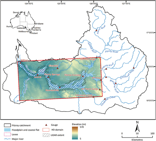
The Fitzroy catchment experiences a semi-arid climate with a mean annual rainfall of 550 mm. The rainfall is characterized by a highly distinctive wet season (November to April) and dry season (May to October). Rivers and creeks in the Fitzroy catchment are mostly ephemeral except the Fitzroy River downstream of Fitzroy Crossing where flow varies between perennial and intermittent. Intense seasonal rains from December to April create localized flooding and inundate large areas across the Fitzroy and Margaret rivers. A major source of flood water is the inflow from headwater catchments upstream of Dimond Gorge and Mt Krauss, while about 15% of flood water is generated from local rainfall. Floods in the Fitzroy catchment mostly occur in the period from January to March (88%) with the highest in February (38%). Since 1980, there have been 23 floods ranging from an annual exceedance probability (AEP) of 1–50 years.

3. Data

3.1. Catchment data

3.1.1. Topography

Land surface elevation is an essential input to the HD model, which is often a raster digital elevation model (DEM). Topography governs direction and velocity of flow between modelling grids. We have used two sets of topography data: 1-m resolution LiDAR (Light Detection And Ranging) data was used for the rivers and riparian zones and 30-m resolution SRTM (Shuttle Radar Topography Mission) data for the remainder of the floodplain. The modelling domain covered an area of 3.6 × 10⁴ km² and the area covered by LiDAR is approximately 0.6 × 104 km² (16% of the total area) (Figure 1).

3.1.2. Hydraulic roughness

Land cover which provides resistance to the propagating flood wave is an essential input to HD modelling. We have used several sources of land cover data to estimate hydraulic roughness such as satellite imagery, aerial photos, topographic mapping and Google Earth imagery. At first, a 30 m resolution gridded land cover map was produced by categorizing land cover into bare soil, river, wetland, riparian vegetation, savannas, shrubs and tropical woodlands. Each land cover grid was then replaced with a corresponding hydraulic roughness coefficient (n) using recommended values in published literature (e.g. Duan et al. 2018; LWA 2009; Prior et al. 2021). Roughness coefficients were adjusted during model calibration to produce the best match between observed and modelled water level and discharge along the rivers and across floodplains.

3.1.3. Flow

Streamflow and water level are two important inputs to the HD model configuration and calibration. These data were obtained from the Department of Water of the Government of Western Australia. Daily streamflow at Christmas Creek, Dimond Gorge and Mt Krauss were used to specify inflow from upstream catchments, and the only downstream boundary was specified using daily water levels at Willare (Figure 1). Water levels at Fitzroy Barrage, Fitzroy Crossing, Looma and Noonkanbah gauging sites were used to calibrate model parameters (e.g. roughness coefficient and eddy viscosity). Streamflow data were used to identify relatively recent flood events in the Fitzroy floodplain that were suitable for HD modelling and captured by earth observation sensors. Based on the availability of satellite data, we have selected five floods to evaluate modelled inundation. The magnitude of the selected floods varies from 1 in 5 to 1 in 25 years exceedance probability (Table 2).

Table 2. Characteristics of the recent flood events in the Fitzroy floodplain (ARI = annual recurrence interval).

Start Date	End Date	Duration (days)	Maximum Flow (m^3/s)	Maximum Flow Date	ARI
15/02/2001	14/03/2001	28	6080.83	21/02/2001	10
20/02/2002	7/03/2002	16	15456.89	24/02/2002	25
25/02/2011	29/03/2011	33	14138.57	16/03/2011	24
8/02/2017	22/02/2017	15	6662.36	17/02/2017	16
3/03/2020	8/03/2020	6	5076.32	4/03/2020	5

3.2. Earth observation data

The two MODIS sensors (onboard the TERRA and AQUA platforms since 2000 and 2002, respectively) acquire daytime images over Australia in the morning (TERRA) and afternoon (AQUA). The spatial resolution of MODIS surface reflectance data ranges from 250 m to 1000 m, depending on wavelength (Salomonson, Barnes, and Masuoka 2006). Daily images of the surface reflectance from only the TERRA MODIS sensor (MOD09GA) were used here. This is because of failure of detectors that produce Band 6 on the AQUA sensor, resulting in stripes in the data (Gladkova et al. 2012). Daily MODIS surface reflectance (MOD09GA) was downloaded from NASA’s Earth Data Search website (NASA 2022).

Landsat data have a spatial resolution of 30 m pixels (Wulder et al. 2019). Landsat images are available every 16 days from a single sensor. This becomes more frequent along the edge where the swaths overlap, or with two sensors in orbit, but reduces due to cloud cover and missing data. The archive of Landsat data (Landsat 5 Thematic Mapper, Landsat 7 Enhanced Thematic Mapper, and Landsat 8 Operational Land Imager) is available from Digital Earth Australia (DEA). The DEA provides consistent pre-processing of Landsat data (including atmospheric correction and Bidirectional Reflectance Distribution Function (BRDF) correction) to an analysis-ready level for the Australian continent (Dhu et al. 2017).

The Sentinel-2 sensors are part of the Copernicus Programme by the European Space Agency (ESA). These sensors provide a fine spatial resolution (10–20 m), with observations every 5–10 days. Sentinel-2A data are available from 2015, with more frequent coverage following the launch of Sentinel-2B in 2017 (Phiri et al. 2020). Sentinel-2 data are also provided as BRDF-corrected surface reflectance from DEA.

The S-NPP VIIRS instrument (which will now be called VIIRS) was launched in 2011 and has similar characteristics to MODIS. VIIRS provides daily surface reflectance at a similar spatial resolution to MODIS (375 m pixels for the reflectance bands used in this study), with an afternoon daytime overpass time (Xiong et al. 2016). Daily VIIRS (VNP09GA) were downloaded from NASA’s Earth Data Search website (NASA 2022).

Sentinel-1 consists of two SAR sensors, Sentinel-1A (launched in 2014) and Sentinel-1B (launched in 2016) (Potin et al. 2016). Their common Interferometric Wide Swath mode provides radar backscatter measurements at a pixel size of 10 m, with a spatial resolution of 20 × 22 m, and is available every 6–12 days (although acquisition frequency has been reduced to 12 days following issues with the Sentinel-1B instrument; ESA 2022). Sentinel-1 data were downloaded from the Sentinel Australasia Regional Access Hub (Australian Government 2022).

NovaSAR-1 is an S-band (3.2 GHz; wavelength 9.4 cm) SAR satellite designed and built by Surrey Satellite Technology Ltd, UK. Although data are not routinely acquired, the CSIRO is able to task imagery over Australia (Held et al. 2019). All NovaSAR-1 data are freely available from the CSIRO data portal (CSIRO 2022) and will soon be released in an analysis-ready format (following the Committee on Earth Observation Satellites Analysis Read Data for Land (CARD4L) recommendation of normalized radar backscatter (CARD4L 2022).

All remote sensing imagery for Landsat, MODIS, Sentinel-2, VIIRS, Sentinel-1 and NovaSAR-1 within the flood dates (Table 2) were downloaded for the Fitzroy River HD model domain. Optical imagery with a large proportion of cloud cover was removed from further analysis, however some cloud cover was allowed if the remaining pixels provided a clear view of inundation somewhere within the floodplain. The number of remote sensing scenes used in this study is shown in Table 3. All imagery were resampled to a pixel size of 20 m (the finest spatial resolution of the remote sensing data), allowing for a direct pixel-to-pixel comparison between remote sensing and HD model inundation maps.

Table 3. Number of scenes available from each sensor for each flood event.

Start date	End Date	Landsat	MODIS	Sentinel-2	Sentinel-1	NovaSAR-1	VIIRS
15/02/2001	14/03/2001	2	11
20/02/2002	7/03/2002		8
25/02/2011	29/03/2011	1	8
8/02/2017	23/02/2017	2	5	1	2		6
3/03/2020	11/03/2020	1	6	3	2	1	8

4. Methods

4.1. Hydraulic modelling

The HD modelling was conducted using a two-dimensional flexible mesh flood inundation model, commonly known as MIKE21 FM (DHI 2016). The modelling domain was divided into four zones using different sizes of mesh, with the smallest mesh for rivers and the largest mesh for areas not usually subjected to inundation (Figure 1). The model consisted of approximately 1.62 million triangular mesh, with three inflow boundaries at Dimond Gorge, Mt Krauss and Christmas Creek and a water-level boundary at Willare (Figure 1). Daily discharge was used at three inflow boundaries (Dimond Gorge, Mt Krauss and Christmas Creek), and water level was specified at Willare (Figure 1).

Model boundaries were specified at a daily time step, and hydrodynamic simulations of flow and water depth were undertaken at 5-s intervals. Irrespective of magnitude, each flood event was run for 5 days of warmup and 35 days of simulation to ensure complete flood recession. CSIRO’s high-performance computing facilities were used to run the models. Each machine consists of 3 GPU (graphic processing unit) cards and 16 CPU (central processing unit) cores. For the current setup, each model run takes about one and a half days of computer time for a 40-day flood event. To reduce data volume, model outputs were recorded at six hourly time steps: 6am, midday, 6pm and midnight, which was deemed sufficient for the inundation analysis.

4.2. Producing water maps from satellite data

4.2.1. Water maps from optical data

Two of the most commonly used and validated methods of mapping surface water within Australia are the modified Normalized Difference Water Index (mNDWI) by Xu (2006) and a water index by Fisher, Flood, and Danaher (2016) (which will be called FWI). Ticehurst, Teng, and Sengupta (2022) utilized these indices, along with the Tasseled Cap Wetness index (Dunn et al. 2019), applying them within the water environments where they perform best. This method was used here for the Fitzroy floodplain, which, given its environment, uses the maximum of mNDWI and FWI (Max_{fwi_ndwi}):

(1) $\mathrm{M}\mathrm{a}{\mathrm{x}}_{\mathrm{f}\mathrm{w}\mathrm{i}\mathrm{\_}\mathrm{n}\mathrm{d}\mathrm{w}\mathrm{i}}=\left(\mathrm{m}\mathrm{N}\mathrm{D}\mathrm{W}\mathrm{I}>0.0\right)\mathrm{V}\hspace{0.17em}\hspace{0.17em}(\mathrm{F}\mathrm{W}\mathrm{I}>0.63)$(1)

where:

(2) $\mathrm{F}\mathrm{W}\mathrm{I}=\hspace{0.17em}1.7204+171\mathrm{x}\mathrm{g}\mathrm{r}\mathrm{e}\mathrm{e}\mathrm{n}+3\mathrm{x}\mathrm{r}\mathrm{e}\mathrm{d}-70\mathrm{x}\mathrm{N}\mathrm{I}\mathrm{R}-\hspace{0.17em}45\mathrm{x}\mathrm{S}\mathrm{W}\mathrm{I}\mathrm{R}1\hspace{0.17em}-71\mathrm{x}\mathrm{S}\mathrm{W}\mathrm{I}\mathrm{R}2$(2)

(3) $\mathrm{m}\mathrm{N}\mathrm{D}\mathrm{W}\mathrm{I}=\frac{\mathrm{g}\mathrm{r}\mathrm{e}\mathrm{e}\mathrm{n}-\mathrm{S}\mathrm{W}\mathrm{I}\mathrm{R}1}{\mathrm{g}\mathrm{r}\mathrm{e}\mathrm{e}\mathrm{n}+\mathrm{S}\mathrm{W}\mathrm{I}\mathrm{R}1}$(3)

NIR is the near-infrared band. SWIR1 and SWIR2 are the Short Wave Infrared bands around the 1500–1600 nm and 2100–2200 nm wavelengths, respectively.

Since Max_{fwi_ndwi} uses the combination of the FWI and mNDWI indices, it allows for the identification of different coloured water (Fisher, Flood, and Danaher 2016). Max_{fwi_ndwi} was used to produce water maps from all the optical images (Landsat, MODIS, Sentinel-2 and VIIRS) to allow a direct comparison.

4.2.2. Water maps from Synthetic Aperture Radar data

The Sentinel-1 data were first terrain corrected and processed to orthorectified normalized radar backscatter using the European Space Agency SNAP toolbox. NovaSAR-1 was provided as terrain corrected and orthorectified normalized radar backscatter (processed using GAMMA software). The backscatter from both the Sentinel-1 and NovaSAR-1 images was converted from linear to decibels (dB) and a 3 × 3 Refined Lee filter applied to reduce speckle effects.

Applying a single threshold to a co-polarized band of SAR backscatter (in this case VV) is a common method for identifying surface water extent due to the low backscatter over open surface water (Bioresita et al. 2019). It requires a strong bimodal distribution of the pixel values, separating the low backscatter of surface water from land. This was achieved by selecting a subset within each SAR image that contained a good representation of both inundated and dry pixels (Bioresita et al. 2018 suggests at least 10% surface water) such that the two modes are visible in the histogram (Islam and Meng 2022). For SAR images covering the lower floodplain, this subset was located between Looma and Fitzroy Barrage (Figure 1), and for those further upstream this subset was located at Fitzroy Crossing. Otsu’s threshold method (Otsu 1979) was then used to automatically select a backscatter threshold. Values below this threshold are classified as water across the whole SAR image.

Low backscatter due to speckle and steep terrain (Islam and Meng 2022), as well as smooth ground (O’Grady, Leblanc, and Gillieson 2013) result in dry pixels mis-classified as water. This can be improved by masking regions of steep terrain and removing small clumps of pixels classified as water (Islam and Meng 2022). Hence, two further steps were applied: a sieve filter (available in QGIS software) was used to remove small clumps of classified water pixels less than 10 in size (since these are not usually part of a large, inundated area); and a floodplain mask was applied using MrVBF (Gallant and Dowling 2003) allowing pixels on steeper terrain (with MrVBF<5) to be removed. The MrVBF algorithm uses the SRTM DEM to categorize topography based on the degree of ‘valley bottom flatness’, resulting in an index ranging from 0 (steep slopes) to 8 (flat valley).

4.2.3. Image assessment

All inundation maps for the images within the flood dates were directly compared to the HD model maps for the same date (and similar matching time). Given that the HD model was calculated every 6 hours (6am, midday, 6pm, midnight), the midday HD model extent was used for the optical images (which were acquired around 10–10.30am). For Sentinel-1 (with a local acquisition time ~7am) the 6am HD model extents were used, and for NovaSAR-1 (acquired ~9.30pm) it was midnight. All remote sensing images acquired on the same date were also compared, despite their different acquisition times.

All comparisons were made using the user’s accuracy (UA; Equation 4(4) $UA=TP/\left(\mathrm{T}\mathrm{P}+\mathrm{F}\mathrm{P}\right)$(4) ), producer’s accuracy (PA; Equation 5(5) $PA=\mathrm{T}\mathrm{P}/\left(TP+FN\right)$(5) ) and F1 score (Equation 6(6) $F1\mathrm{\_}score=2\hspace{0.17em}\times \mathrm{P}\mathrm{A}\times \mathrm{U}\mathrm{A}/\left(PA+UA\right)$(6) ). All null pixels from the remote sensing data were omitted from the analysis.

(4) $UA=TP/\left(\mathrm{T}\mathrm{P}+\mathrm{F}\mathrm{P}\right)$(4)

(5) $PA=\mathrm{T}\mathrm{P}/\left(TP+FN\right)$(5)

(6) $F1\mathrm{\_}score=2\hspace{0.17em}\times \mathrm{P}\mathrm{A}\times \mathrm{U}\mathrm{A}/\left(PA+UA\right)$(6)

where TP (true positive) is the number of water pixels in agreement, FP (false positive) is the number of dry pixels incorrectly mapped as water, and FN (false negative) is the number of water pixels incorrectly mapped as dry (Maxwell and Warner 2020).

For the remote sensing image – HD model comparisons, the HD water extents were considered the ‘true’ pixels. For the remote sensing – remote sensing image comparisons, one dataset was nominated as ‘true’ pixels to enable calculation of PA and UA: MODIS was considered the ‘true’ pixels when compared to the other datasets; VIIRS was considered the ‘true’ pixels when compared to Sentinel-2, Sentinel-1 and NovaSAR-1; and Sentinel-2 was considered the ‘true’ pixels when compared to NovaSAR-1. Selection of the remote sensing data considered as ‘true’ is arbitrary since it was just to allow additional comparisons, in relation to omission and commission errors, of the water extents.

5. Results

5.1. Comparison of remote sensing data with hydrodynamic model output

Figure 2 shows the comparison of a selection of remote sensing images with the HD model for the same dates. For the Landsat – HD comparison, the best agreement has an F1 score of 0.83 on 26 February 2001 (Figure 2a) occurring when inundation was extensive around the lower floodplain. The next highest F1 score of 0.76 also occurred when the water had extended beyond the river channel in the lower floodplain (on 22 February 2017; Figure 2b). The poorest agreement has an F1 score of 0.26 (on 23 March 2017; Figure 2c) in the upper catchment of the HD model domain at the very end of the flood event when much of the water had subsided.

Figure 2. Spatial comparison of Landsat (LS), MODIS (MD), Sentinel-1 (S1), NovaSAR-1 (N1), Sentinel-2 (S2) and VIIRS (VI) with the hydrodynamic (HD) model water extent for different flood dates (F1 score is shown in brackets next to date, RS = remote sensing data).

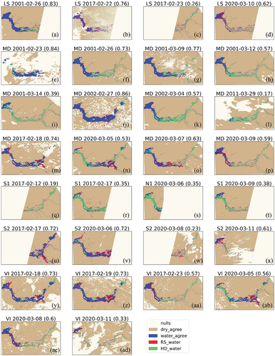
For the MODIS – HD comparisons there is strong agreement with an F1 score of 0.86 (on 27 February 2002; Figure 2j), occurring when the flood extent was at its greatest. Another comparison also showed strong agreement with an F1 score of 0.84 (on 23 February 2001; Figure 2e). The poorest agreement has an F1 score of 0.17 (on 29 March 2011; Figure 2l) which is at the end of the flood event when little floodwater is visible in the MODIS water maps compared to the HD model. The other poor F1 scores also occur at the end of flood events when the river width has narrowed, and the water has subsided in the MODIS water maps.

For the Sentinel-2 – HD comparisons there is reasonable agreement for three of the four images, with the highest F1 score of 0.72 (on 17 February 2017 and 6 March 2020; Figure 2u,v respectively). Poor agreement occurs in one image pair (F1 score of 0.23, on 8 March 2020; Figure 2w) which is upstream of the floodplain when flood extent is small.

For the VIIRS – HD comparisons the highest F1 score is 0.73 (on 19 February 2017; Figure 2z) with the poorest agreement (F1 score of 0.33; on 11 March 2020; Figure 2ad) occurring at the end of the flood event.

Overall, for the optical remote sensing data, the best agreements with the HD model occur when the flood is at its largest. The lowest agreements happen near the end of the flood events.

The SAR – HD comparisons were mostly of poor agreement (F1 scores ranging from 0.19 to 0.38), with the best agreement occurring for Sentinel-1 (on 9 March 2020; Figure 2t). These poor agreements do not appear to be related to the size of flood event, however the individual comparisons in Figure 2 show areas of agreement are distributed throughout the HD model domain in the larger bodies of water.

For each sensor, the mean PA and UA, and mean, minimum and maximum F1 scores were calculated when compared to the HD model extent (Table 4). The Landsat water maps have the highest agreement to the HD model extents with a mean F1 score of 0.65. Half of the image pairs show good agreement with F1 scores above 0.76. The mean PA (0.59) is lower than the mean UA (0.76) indicating the HD model is identifying more water than the Landsat water maps. The MODIS and VIIRS show moderate agreement with a mean F1 score of 0.61 and 0.58, respectively. For the MODIS – HD image pairs, 13 of the 38 had substantial agreement with F1 scores above 0.7. However, Landsat, MODIS and VIIRS all show good agreement with the HD model for some of the individual images, with the best agreements occurring when the flood is at its largest.

Table 4. Summary results for remote sensing data compared to hydrodynamic model.

Sensor	Number of images	Mean PA	Mean UA	Mean F1	Min F1	Max F1
Landsat	6	0.59	0.76	0.65	0.26	0.83
MODIS	38	0.51	0.87	0.61	0.17	0.92
Sentinel-2	4	0.58	0.58	0.57	0.23	0.72
VIIRS	14	0.51	0.68	0.58	0.33	0.73
NovaSAR-1	1	0.22	0.77	0.35	0.35	0.35
Sentinel-1	4	0.20	0.69	0.31	0.19	0.38

For Sentinel-2, the mean F1 score is 0.57, and the mean PA is the same as the mean UA (0.58) indicating an even amount of over-mapping and under-mapping of water compared to the HD model. Both the SAR sensors show poor agreement with the HD model water extents with a mean F1 score of 0.31 for Sentinel-1 and 0.35 for the NovaSAR-1 image. The mean PA is much lower than the mean UA for both Sentinel-1 and NovaSAR-1 indicating that the SAR water maps identify much less water than the HD model. The agreement is best in the open floodplain areas and in the deep river channel.

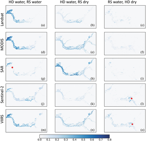
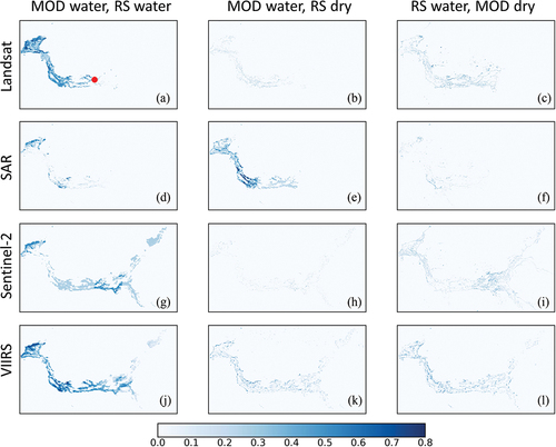
Figure 3 summarizes the spatial agreement across the floodplain of the remote sensing images with the HD model for the common dates. It shows proportion of times where: the remote sensing identifies water in the same pixels as the HD model (left column); the HD model identifies water and the remote sensing does not (middle column); and the remote sensing identifies water and the HD model does not (right column). The best agreement for the Landsat – HD (Figure 3a) and MODIS − HD (Figure 3d) image pairs occurs in the lower half of the floodplain (along the eastern side). The best agreement for the SAR – HD image pairs occurs along the lowest section where the water spreads along the floodplain downstream of Fitzroy Barrage (red dot in Figure 3g). Agreement for the Sentinel-2 – HD (Figure 3j) and VIIRS – HD (Figure 3m) image pairs is more evenly distributed across the floodplain. The HD model is identifying more water across the whole floodplain compared to MODIS (Figure 3e), SAR (Figure 3h) and VIIRS (Figure 3n). For MODIS and VIIRS, this is most likely because of their low spatial resolution compared to the HD model. Only Sentinel-2 and VIIRS are identifying a notable amount of additional water compared to the HD model, particularly near the junction of Christmas Creek and Fitzroy River in the southwest of the HD model domain (red dots in Figure 3l,o respectively).

Figure 3. Spatial comparison of proportion of agreement (‘HD water, RS water’) and disagreement (‘HD water, RS dry’ and ‘RS water, HD dry’) for Landsat, MODIS, SAR (Sentinel-1 and NovaSAR-1), Sentinel-2 and VIIRS with the hydrodynamic model (HD) water extent as calculated from all common flood dates (RS = remote sensing data). The red dots show the location of Fitzroy Barrage (Figure 3g) and the junction of Fitzroy River and Christmas Creek (Figure 3l and Figure 3o).

The HD model was used to identify date of maximum extent of a flood event. To allow for the fact that remote sensing data are unlikely to capture the maximum extent, the dates within 80% of the flood peak are used. If only this stage of the flood is considered, the F1 scores improve somewhat for the optical data (Table 5). The Landsat – HD mean F1 score increases from 0.65 to 0.80. The MODIS – HD mean F1 score increases from 0.61 to 0.70, and the Sentinel-2 – HD mean F1 score also increases from 0.57 to 0.72. The mean F1 score for the VIIRS – HD image pairs increases marginally from 0.58 to 0.61. However, this smaller improvement from the VIIRS – HD image pairs, compared to the MODIS – HD image pairs, may be more related to the size of the flood events available for assessing VIIRS (since the 2017 and 2020 events are much smaller than those of 2002 and 2011). There is no change for the NovaSAR-1 – HD image pair, and the Sentinel-1 – HD image pair increases slightly (0.29 to 0.35) but still remains with a low mean F1 score.

Table 5. Summary results for remote sensing data compared to the hydrodynamic model for the dates close to flood peak (i.e. ±80% of flood peak).

Sensor	Number of images	Mean PA	Mean UA	Mean F1	Min F1	Max F1
Landsat	2	0.81	0.81	0.80	0.77	0.83
MODIS	13	0.62	0.82	0.70	0.53	0.92
Sentinel-2	2	0.77	0.68	0.72	0.72	0.72
VIIRS	8	0.55	0.69	0.61	0.51	0.73
NovaSAR-1	1	0.22	0.77	0.35	0.35	0.35
Sentinel-1	3	0.23	0.74	0.35	0.32	0.38

5.2. Comparison of remote sensing data with other coincident remote sensing data

Individual remote sensing images acquired on the same day from different sensors were spatially compared and their F1 scores calculated. Figure 4 shows the spatial comparison of a selection of remote sensing water maps with the MODIS water maps (since these were the most numerous of the sensors) to demonstrate the differences seen between the sensors.

Figure 4. Spatial comparison of Landsat (LS), Sentinel-2 (S2), VIIRS (VI), Sentinel-1 (S1) and NovaSAR-1 (N1) with MODIS water extent for common flood dates (F1 score is shown in brackets next to date, RS = remote sensing data being compared to MODIS).

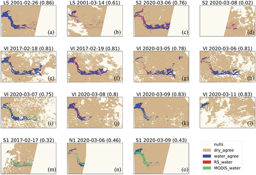
For the Landsat – MODIS image pairs, there was strong agreement with an F1 score of 0.86 (on 26 February 2001; Figure 4a) when flood extent was largest. The lowest agreement had an F1 score of 0.61 (on 14 March 2001; Figure 4b) when flood extent had reduced.

For the MODIS – VIIRS image pairs, the agreement was not related to the size of inundation extent since the best results occurred not only when the flood was at its peak (with an F1 score of 0.81 on 19 February 2017; Figure 4f) but also at the very end of a flood event (with an F1 score of 0.83 on 11 March 2020; Figure 4l). The lowest agreement had an F1 score of 0.75 (on 7 March 2020; Figure 4i) and showed that MODIS identified more water than VIIRS. This may be partly related to the different acquisition times during the flood’s recession (MODIS ~10am, VIIRS ~1.30pm).

For the MODIS – Sentinel-2 image pairs, the highest F1 score was 0.76 (on 6 March 2020; Figure 4c) and the lowest F1 score (0.02) showed extremely poor agreement (on 8 March 2020; Figure 4d). This was mostly due to the difference in spatial resolution of the sensors. This image pair only covers the upstream section of the river when the inundation extent was low, so the MODIS was not detecting water in its larger pixels.

For the MODIS – SAR image pairs, there was low-to-moderate agreement for all image pairs. The best agreement was found for NovaSAR-1 with an F1 score of 0.46 (on 6 March 2020; Figure 4n). The lowest F1 score was 0.32 for Sentinel-1 (on 17 February 2017; Figure 4m). The SAR data agree with MODIS for the larger bodies of water rather than the narrow river channels.

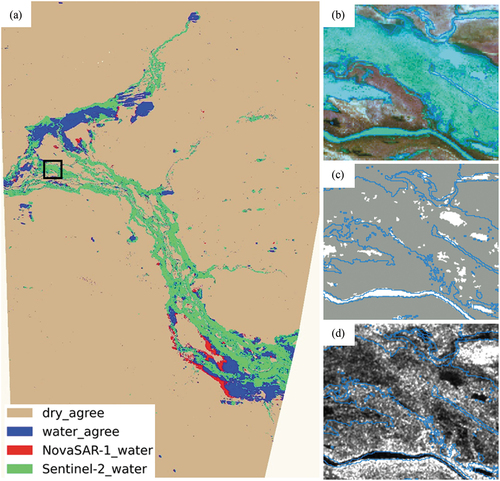
For the NovaSAR-1 – Sentinel-2 image pair (Figure 5a; noting there were no image pairs from Sentinel-1), there was moderate agreement for the one date (F1 score of 0.46). Both NovaSAR-1 and Sentinel-2 have a similar spatial resolution; however, the NovaSAR-1 is not capturing as much water as was identified in Sentinel-2. To further illustrate this, flood extent (as derived from the Sentinel-2 image using Max_{fwi_ndwi}) is outlined in blue in Figure 5b,c,d. Figure 5b uses the Red, Green and SWIR-2 band to show flooded water, as well as shallow flooded vegetation (which can be seen by the speckled texture in the water). The NovaSAR-1 water map (Figure 5c) is identifying water where flooded vegetation is not visible, including the flooded river channel running along the bottom of the image. The NovaSAR-1 VV backscatter image (Figure 5d) shows the backscatter is greater in the areas where there is scattered, partially submerged vegetation, compared to inundated areas void of vegetation.

Figure 5. (a) Spatial comparison of Sentinel-2 and NovaSAR-1 water extent for 6^th March 2020. (b) Sentinel-2 image (RGB = Red, Green, SWIR-2 bands), (c) NovaSAR-1 water map, and (d) NovaSAR-1 VV image for subset area (black square).

There were 29 image pairs acquired on the same day from different remote sensing instruments. The number of image pairs, as well as mean PA, mean UA, and mean, minimum and maximum F1 scores are shown in Table 6. There were no image pairs for Landsat – Sentinel-2 or Sentinel-1 – Sentinel-2. The MODIS – Landsat and MODIS – VIIRS image pairs had substantial agreement (with mean F1 scores of 0.76 and 0.80 respectively). For MODIS – VIIRS image pairs, there was strong agreement for most dates with seven of the ten having an F1 score above 0.8, and the remaining three with an F1 score above 0.75. The MODIS – Sentinel-2 and VIIRS – Sentinel-2 image pairs had a moderate agreement (mean F1 score of 0.57 and 0.56, respectively). However, for both the MODIS – Sentinel-2 and VIIRS – Sentinel-2 image pairs, there was substantial agreement for three out of the four dates, with F1 scores ranging from 0.72 to 0.77 and from 0.68 to 0.75, respectively. For the VIIRS – SAR image pairs there was moderate agreement for two out of the four dates: one from NovaSAR-1 and one from Sentinel-1 (F1 scores of 0.45 and 0.41 respectively). The other two images, both Sentinel-1, showed poor agreement with VIIRS (F1 scores below 0.32).

Table 6. Summary results for remote sensing data compared to other coincident remote sensing data.

Sensors	Number of images	Mean PA	Mean UA	Mean F1	Min F1	Max F1
MODIS – Landsat	4	0.87	0.68	0.76	0.61	0.86
MODIS – VIIRS	10	0.81	0.80	0.80	0.75	0.83
MODIS – Sentinel-2	4	0.91	0.48	0.57	0.02	0.76
MODIS – Sentinel-1	4	0.24	0.75	0.36	0.32	0.43
MODIS – NovaSAR-1	2	0.38	0.60	0.46	0.46	0.46
VIIRS – Sentinel-2	1	0.87	0.47	0.56	0.08	0.75
VIIRS – Sentinel-1	3	0.22	0.67	0.34	0.28	0.41
VIIRS – NovaSAR-1	1	0.34	0.64	0.45	0.45	0.45
Sentinel-2 –NovaSAR-1	1	0.22	0.84	0.46	0.46	0.46

The mean UA for the MODIS – Landsat and MODIS – Sentinel-2 image pairs are lower than the mean PA, indicating that MODIS is under-mapping water more than the other sensor (Table 6). The same result is also seen in the VIIRS – Sentinel-2 comparison. This is largely due to the different spatial resolution of the sensors and the fine spatial inundation extent of the receding flood water. The MODIS – VIIRS image pairs have similar mean UA (0.80) and mean PA (0.81) meaning they are mapping similar extents. Similar to the MODIS – SAR image pairs, the VIIRS – SAR image pairs have a low to moderate mean F1 score (lower than 0.48). All the image pairs containing SAR have a much lower mean PA than mean UA indicating SAR is under-mapping water extent compared to the other sensors.

Figure 6 summarizes the spatial agreement of the MODIS water maps with the other remote sensing water maps (Landsat, SAR, Sentinel-2 and VIIRS) for the common dates. It shows proportion of times where: MODIS identifies water in the same pixels as the other remote sensing water map (left column); the MODIS identifies water and the other remote sensing water map does not (middle column); and the other remote sensing water map identifies water and the MODIS does not (right column). The MODIS – Landsat image pairs show the highest agreement within the lower half of the floodplain on the eastern side, downstream from Noonkanbah (red dot in Figure 6a), while the MODIS – SAR image pairs show agreement around the larger bodies of water within the lower floodplain (Figure 6d). The MODIS – Sentinel-2 and MODIS – VIIRS image pairs show agreement distributed across the whole floodplain (Figure 6g,j respectively). The MODIS – SAR image pairs show the largest difference, where MODIS identifies a lot more water than SAR (Figure 6e), while SAR is not identifying much more water than MODIS (Figure 6f). Landsat and Sentinel-2 show more water than MODIS across the whole floodplain (Figure 6c,i), although this difference is low and mostly related to the lower spatial resolution of the MODIS. The VIIRS and MODIS are showing small differences across the whole floodplain (Figure 6k,l), which is possibly related to the different observation times (MODIS in the morning and VIIRS in the afternoon).

Figure 6. Spatial comparison of proportion of agreement (‘MOD water, RS water’) and disagreement (‘MOD water, RS dry’ and ‘RS water, MOD dry’) for Landsat, SAR (Sentinel-1 and NovaSAR-1), Sentinel-2 and VIIRS with the MODIS water extent as calculated from all common flood dates (RS = all remote sensing data except MODIS – which it is being compared to). The red dot shows the location of Noonkanbah in Figure 6a.

6. Discussion

The main strength of hydrodynamic modelling is that it is directly linked with hydrology and can produce inundation information at a desired spatial (e.g. 5 m) and temporal (e.g. sub-daily) resolution with high accuracy. The main limitation of hydrodynamic modelling is that it requires large input data sets. Moreover, the configuration, simulation and calibration of the model is time-consuming. To our knowledge, comparison of a range of remote sensing-derived inundation extents with a HD model is a novel approach, and enables accuracy assessments to be made even when remote sensing observations are not coincident.

The agreements between the optical imagery and the HD model are better during the flood peak rather than the recession where the HD model identifies more water. Many factors influence the accuracy of the remote sensing and HD model image pairs, including the timing of image acquisition in relation to the stage of the flood event, as well as the area covered by the imagery (since the comparisons tend to be better in the lower floodplain where inundation is more extensive).

The lower spatial resolution of the MODIS/VIIRS means it cannot detect the finer river channel, and sections of braided river, compared to the HD model and the higher-resolution remote sensing imagery. These lower spatial resolution sensors cannot detect changes in inundation extent along narrow rivers or small or irregular-shaped waterbodies (Wang et al. 2022), further explaining why results improved in optical imagery during flood peak times. While the VIIRS results, when compared to the HD model, were poorer than for MODIS, the common dates of the VIIRS and MODIS showed similar F1 scores with the HD model. Furthermore, the MODIS – VIIRS image pairs showed substantial agreement with a mean F1 score of 0.8, hence VIIRS may also be a suitable sensor for large flood events. Huang et al. (2015) also concluded that MODIS and VIIRS provided similar extents for a large lake, validating this with Landsat 8.

The SAR data are mapping less water than the other remote sensing datasets and the hydrodynamic model. One reason for this is because SAR backscatter increases in turbulent water, which may be due to vegetation scattered within the shallow inundated areas, making it difficult to distinguish from other surface features. In cases where inundation occurs under reasonably dense vegetation, resulting in a strong increase in backscattering due to double-bounce scattering, these areas can be identified using a different threshold (Cazals et al. 2016). The situation in this study is more complicated as illustrated in Figure 5, where an increase in backscatter in the inundated areas is not indicative of the strong double-bounce response that enables flooded vegetation to be easily identified from its surrounds (Rosenqvist et al. 2007). The small size of the flood events in 2017 and 2020, when SAR data were available, resulted in shallower inundation depth and hence more influence on backscatter from low vegetation. Souza et al. (2022) also found that optical imagery (Landsat-8 and Sentinel-2) mapped water extent better than SAR in areas where water features, such as inlet branches, were more complex. Levin and Phinn (2022) compared PlanetScope and Capella-Space X-band imagery captured at the peak of a flood event in Brisbane, Australia, finding the SAR identified less flood water due to vegetation and buildings. Despite these findings, SAR sensors have demonstrated their ability to map smooth open surface water.

While NovaSAR-1 is not a global dataset, applying the S-band SAR to inundation mapping contributes to the very limited body of research (such as Bhardwaj, Saini, and Chatterjee 2021; Liang et al. 2016) in preparation for the NiSAR (S-band and C-band) mission scheduled for 2024 (NASA 2023). While we could not directly compare the Sentinel-1 and NovaSAR-1 inundation extents since observations were not coincident, comparison with the HD model enabled their accuracy to be assessed. Results showed that both SARs were able to identify the larger open bodies of water and flooded river channels, but not shallow inundation mixed with scattered vegetation. Similar results were found for Ramsey, Rangoonwala, and Bannister (2013) who report mapping accuracies with L- and C-bands that were lower for shallow water depths compared to deep water. Manavalan, Rao, and Krishna Mohan (2017) reported inundation extent in deeply flooded agricultural areas was greater from L-band compared to C-band, since flooded vegetation can appear smoother at the longer wavelength, however our study was unable to detect any noticeable difference between S-band and C-band.

Apart from the NovaSAR-1 data, all the remote sensing data used here are freely available covering most of the globe. Given the simplicity of the methods used to map surface water in the optical remote sensing imagery, they can be applied and have been validated across a diverse range of environments (Max_{fwi_ndwi} in south-east Australia, Ticehurst, Teng, and Sengupta 2022; FWI in eastern Australia, Fisher, Flood, and Danaher (2016); mNDWI in the Yangtze River Basin, Li et al. (2013)). The SAR backscatter threshold method has already been utilized in many different water mapping applications (e.g. Kavats, Khramov, and Sergieieva 2022; Brown, Hambidge, and Brownett 2016), after adapting the threshold to individual sites. The topography mask applied to the SAR water extents was extracted from MrVBF, which is only available for Australia, however the SRTM data used to derive it is a global product. Furthermore, other topography information can be applied depending on the environment and available data (e.g. Wang et al. 2022; Islam and Meng 2022). While comparisons of water extent derived from different remote sensing data have been reported for large lakes (e.g. MODIS, VIIRS and Landsat, Huang et al. 2015; Sentinel-1, Landsat-8 and Sentinel-2, Souza et al. 2022) and floods (PlanetScope, Capella-Space X-band and VIIRS night-time brightness imagery, Levin and Phinn 2022) we are not aware of other comparisons made with such a large range of sensors for flood events.

The same method and index threshold have been used to map surface water for all the optical remote sensing imagery. While the agreement between the optical remote sensing water maps is generally good, the thresholds could be fine-tuned to produce surface water maps with an even stronger agreement. For the SAR data, further analysis on the identification of shallow flood water within scattered vegetation would help improve these comparisons, and methods such as image differencing using the baseline method (Brown, Hambidge, and Brownett 2016), provided a pre-flood image is available, may improve results.

7. Conclusions

In this study, we have gathered, processed and evaluated several sets of near-coincident flood inundation maps derived from optical sensors (Landsat, MODIS, Sentinel-2 and VIIRS), and SAR sensors (Sentinel-1 and NovaSAR-1). Inundation maps derived from satellite imagery were evaluated against an independent data set obtained from hydrodynamic modelling. Among the satellite data, the optical remote sensing data produced a moderate to substantial agreement when compared to the HD model results, with Landsat and MODIS performing the best with mean F1 scores of 0.65 and 0.61, respectively. In contrast, Sentinel-1 and NovaSAR-1 SAR data produced relatively poor agreements with HD model results (mean F1 scores of 0.31 and 0.35 respectively) and the optical remote sensing data (mean F1 scores ranging from 0.34 to 0.46), particularly within scattered vegetation adjacent to the river channel, with better results obtained in open water on the floodplain and in the river channel. This study also showed that Landsat, MODIS, and Sentinel-2 all compare well to the HD model around the peak periods of a flood event with mean F1 scores of 0.80, 0.70 and 0.72, respectively. The results imply that these three sensors can be used interchangeably to identify inundation extent around the peak of a flood event with reasonable confidence, while the VIIRS sensor may also be a suitable sensor for large flood events given it has a high mean F1 score (0.80) when compared to MODIS. This study demonstrates the advantages of using multiple remote sensing technologies for identifying flood events.

Acknowledgements

The authors wish to thank Zheng-Shu Zhou (CSIRO, Data 61) for processing the NovaSAR-1 imagery to an analysis ready format. The authors also thank NASA for free access to the Landsat, MODIS and VIIRS data, and the ESA for free access to Sentinel-1 and Sentinel-2 data. © SSTL 2020 NovaSAR-1™ Level 1 Data. The NovaSAR-1 Data used to produce this research paper was generated by the NovaSAR-1™ satellite owned and operated by Surrey Satellite Technology Limited and provided by CSIRO as authorised licensor of the SSTL Data.

Disclosure statement

No potential conflict of interest was reported by the authors.

Data availability statement

The data that support the findings of this study are available from the corresponding author, CT, upon reasonable request.

References

- Arthington, A. H., R. G. Pearson, P. C. Godfrey, F. Karim, and J. Wallace. 2020. “Integrating Freshwater Wetland Science into Planning for Great Barrier Reef Sustainability.” Aquatic Conservation: Marine & Freshwater Ecosystems 30: 1727–1733. doi:10.1002/aqc.3339.
- Australian Government. 2022. “SARA Sentinel Australasia Regional Access”. https://copernicus.nci.org.au/sara.client/#/home.
- Bhardwaj, A., O. Saini, and R. S. Chatterjee. 2021. “Separability Analysis of Back-Scattering Coefficient of NovaSAR-1 S-Band SAR Datasets for Different Land Use Land Cover (LULC) Classes.” PREPRINT (Version 1) available at Research Square. doi:10.21203/rs.3.rs-854337/v1.
- Bioresita, F., A. Puissant, A. Stumpf, and J. -P. Malet. 2018. “A Method for Automatic and Rapid Mapping of Water Surfaces from Sentinel-1 Imagery.” Remote Sensing 10 (2). doi:10.3390/rs10020217.
- Bioresita, F., A. Puissant, A. Stumpf, and J. -P. Malet. 2019. “Fusion of Sentinel-1 and Sentinel-2 Image Time Series for Permanent and Temporary Surface Water Mapping.” International Journal of Remote Sensing 40 (23): 9026–9049. doi:10.1080/01431161.2019.1624869.
- Boschetti, M., F. Nutini, G. Manfron, P. A. Brivio, and A. Nelson. 2014. “Comparative Analysis of Normalised Difference Spectral Indices Derived from MODIS for Detecting Surface Water in Flooded Rice Cropping Systems.” PLos One 9 (2): e88741. doi:10.1371/journal.pone.0088741.
- Brakenridge, R., and E. Anderson. 2006. “MODIS-Based Flood Detection, Mapping and Measurement: The Potential for Operational Hydrological Applications.” Transboundary Floods Reduce Risks Through Flood Management 72: 1–12.
- Brown, K. M., C. H. Hambidge, and J. M. Brownett. 2016. “Progress in Operational Flood Mapping Using Satellite Synthetic Aperture Radar (SAR) and Airborne Light Detection and Ranging (LiDar) Data.” Progress in Physical Geography: Earth and Environment 40 (2): 196–214. doi:10.1177/0309133316633570.
- CARD4L. 2022. Committee on Earth Observation Satellites, Analysis Ready Data for Land, Normalised Radar Backscatter. https://ceos.org/ard/files/PFS/NRB/v5.5/CARD4L-PFS_NRB_v5.5.pdf.
- Cazals, C., S. Rapinel, P. -L. Frison, A. Bonis, G. Mercier, C. Mallet, S. Corgne, and J. -P. Rudant. 2016. “Mapping and Characterization of Hydrological Dynamics in a Coastal Marsh Using High Temporal Resolution Sentinel-1A Images.” Remote Sensing 8: 570. doi:10.3390/rs8070570.
- CSIRO. 2022. “CSIRO NovaSAR-1 National Facility Datahub”. https://data.novasar.csiro.au/#/home.
- DHI. 2016. MIKE21 Flow Model FM, Hydrodynamic Module, User Guide. Horsholm, Denmark: DHI Water and Environment Pty Ltd. https://manuals.mikepoweredbydhi.help/2017/Coast_and_Sea/MIKE_FM_HD_2D.pdf.
- Dhu, T., B. Dunn, B. Lewis, L. Lymburner, N. Mueller, E. Telfer, A. Lewis, A. McIntyre, S. Minchin, and C. Phillips. 2017. “Digital Earth Australia – Unlocking New Value from Earth Observation Data.” Big Earth Data 1 (1–2): 64–74. doi:10.1080/20964471.2017.1402490.
- Duan, Q., F. Ma, J. You, Z. Zhou, and A. Ye. 2018. “Dynamic Manning’s Roughness Coefficients for Hydrological Modelling in Basins.” Hydrology Research 49 (5): 1379–1395. doi:10.2166/nh.2018.175.
- Dunn, B., L. Lymburner, V. Newey, A. Hicks, and H. Carey. 2019. “Developing a Tool for Wetland Characterisation Using Fractional Cover, Tasseled Cap Wetness and Water Observations from Space”. IGARSS 2019 - 2019 IEEE International Geoscience and Remote Sensing Symposium, 2019, 6095–6097. doi: 10.1109/IGARSS.2019.8897806.
- Dutta, D., J. Alam, K. Umeda, H. Hayashi, and S. Hironaka. 2007. “A Two Dimensional Hydrodynamic Model for Flood Inundation Simulation: A Case Study in the Lower Mekong River Basin.” Hydrological Processes 21 (9): 1223–1237. doi:10.1002/hyp.6682.
- ESA. 2022. “Mission Ends for Copernicus Sentinel-1B Satellite”. The European Space Agency. https://www.esa.int/Applications/Observing_the_Earth/Copernicus/Sentinel-1/Mission_ends_for_Copernicus_Sentinel-1B_satellite.
- FEMA. 2003. “Guidelines and Specifications for Flood Hazard Mapping Partners.” Federal Emergency Management Agency, USA 1.
- Feng, M., J. O. Sexton, S. Channan, and J. R. Townshend. 2015. “A Global, High-Resolution (30-M) Inland Water Body Dataset for 2000: First Results of a Topographic–Spectral Classification Algorithm.” International Journal of Digital Earth 9 (2): 113–133. doi:10.1080/17538947.2015.1026420.
- Feyisa, G. L., H. Meilby, R. Fensholt, and S. R. Proud. 2014. “Automated Water Extraction Index: A New Technique for Surface Water Mapping Using Landsat Imagery.” Remote Sensing of Environment 140: 23–35. doi:10.1016/j.rse.2013.08.029.
- Fisher, A., N. Flood, and T. Danaher. 2016. “Comparing Landsat Water Index Methods for Automated Water Classification in Eastern Australia.” Remote Sensing of Environment 175: 167–182. doi:10.1016/j.rse.2015.12.055.
- Gallant, J. C., and T. I. Dowling. 2003. “A Multiresolution Index of Valley Bottom Flatness for Mapping Depositional Areas.” Water Resources Research 39 (12): 1347. doi:10.1029/2002WR001426.
- Gladkova, M., D. Grossberg, F. Shahriar, G. Bonev, and P. Romanov. 2012. “Quantitative Restoration for MODIS Band 6 on Aqua.” IEEE Transactions on Geoscience & Remote Sensing 50 (6): 2409–2416. doi:10.1109/TGRS.2011.2173499.
- Guerschman, J. P., G. Warren, G. Byrne, L. Lymburner, N. Mueller, and A. Van-Dijk. 2011. MODIS-Based Standing Water Detection for Flood and Large Reservoir Mapping: Algorithm Development and Applications for the Australian Continent. CSIRO: Water for a Healthy Country National Research Flagship Report, Canberra.
- Held, A., Z. -S. Zhou, C. Ticehurst, A. Rosenqvist, A. Parker, and L. Brindle. 2019. “Advancing Australia’s Imaging Radar Capability Under the Novasar-1 Partnership,” IGARSS 2019 - 2019 IEEE International Geoscience and Remote Sensing Symposium, 8370–8373. doi:10.1109/IGARSS.2019.8898623.
- Huang, C., Y. Chen, J. Wu, L. Li, and R. Liu. 2015. “An Evaluation of Suomi NPP-VIIRS Data for Surface Water Detection.” Remote Sensing Letters 6 (2): 155–164. doi:10.1080/2150704X.2015.1017664.
- Islam, M. T., and Q. Meng. 2022. “An Exploratory Study of Sentinel-1 SAR for Rapid Urban Flood Mapping on Google Earth Engine.” International Journal of Applied Earth Observation and Geoinformation 113. doi:10.1016/j.jag.2022.103002.
- Karim, F., J. Pena-Arancibia, C. Ticehurst, S. Marvanek, J. C. Gallant, J. Hughes, D. Dutta, et al.2018Floodplain Inundation Mapping and Modelling for the Fitzroy, Darwin and Mitchell Catchments: A Technical Report from the CSIRO Northern Australia Water Resource Assessment to the Government of Australia, Commonwealth Scientific and Industrial Research Organisation(CSIRO), Canberra 207. doi:10.25919/5b50dfb6c7c0e.
- Karim, F., C. Petheram, S. Marvanek, C. Ticehurst, J. Wallace, and M. Hasan. 2016. “Impact of Climate Change on Floodplain Inundation and Hydrological Connectivity Between Wetlands and Rivers in a Tropical River Catchment.” Hydrological Processes 30: 1574–1593. doi:10.1002/hyp.10714.
- Kavats, O., D. Khramov, and K. Sergieieva. 2022. “Surface Water Mapping from SAR Images Using Optimal Threshold Selection Method and Reference Water Mask.” Water 14: 4030. doi:10.3390/w14244030.
- Khandelwal, A., A. Karpatne, M. E. Marlier, J. Kim, D. P. Lettenmaier, and V. Kumar. 2017. “An Approach for Global Monitoring of Surface Water Extent Variations in Reservoirs Using MODIS Data.” Remote Sensing of Environment 202: 113–128. doi:10.1016/j.rse.2017.05.039.
- Leblanc, M., S. Tweed, A. Van Dijk, and B. Timbal. 2012. “A Review of Historic and Future Hydrological Changes in the Murray–Darling Basin.” Global and Planetary Change 80–81: 226–246. doi:10.1016/j.gloplacha.2011.10.012.
- Levin, N., and S. Phinn. 2022. “Assessing the 2022 Flood Impacts in Queensland Combining Daytime and Nighttime Optical and Imaging Radar Data.” Remote Sens 14: 5009. doi:10.3390/rs14195009.
- Liang, L., Z. Wei, J. Xiaoguang, L. Xianbin, H. -Y. Huo, and Z. Xuehua. 2016. “Water Body Extraction Research Based on S Band SAR Satellite of HJ-1-C.” International Journal of Advanced Remote Sensing and GIS 5 (1): 1514–1523. doi:10.23953/cloud.ijarsg.43.
- Li, W., Z. Du, F. Ling, D. Zhou, H. Wang, Y. Gui, B. Sun, and X. Zhang. 2013. “A Comparison of Land Surface Water Mapping Using the Normalized Difference Water Index from TM, ETM+ and ALI.” Remote Sensing 5: 5530–5549. doi:10.3390/rs5115530.
- Li, J., B. Peng, Y. Wei, and H. Ye. 2021. “Accurate Extraction of Surface Water in Complex Environment Based on Google Earth Engine and Sentinel-2.” PLos One 16 (6): e0253209. doi:10.1371/journal.pone.0253209.
- Li, S., D. Sun, M. D. Goldberg, B. Sjoberg, D. Santek, J. P. Hoffman, M. DeWeese, P. Restrepo, S. Lindsey, and E. Holloway. 2018. “Automatic Near Real-Time Flood Detection Using Suomi-NPP/VIIRS Data.” Remote Sensing of Environment 204: 672–689. doi:10.1016/j.rse.2017.09.032.
- Li, J., and S. Wang. 2015. “An Automatic Method for Mapping Inland Surface Waterbodies with Radarsat-2 Imagery.” International Journal of Remote Sensing 36: 1367–1384. doi:10.1080/01431161.2015.1009653.
- LWA. 2009. An Australian Handbook of Stream Roughness Coefficients, 28. Land and Water Australia, Canberra. http://lwa.gov.au/products/pn30109.
- Manavalan, R., Y. S. Rao, and B. Krishna Mohan. 2017. “Comparative Flood Area Analysis of C-Band VH, VV, and L-Band HH Polarizations SAR Data.” International Journal of Remote Sensing 38 (16): 4645–4654. doi:10.1080/01431161.2017.1325534.
- Martinis, S., A. Twele, and S. Voigt. 2009. “Towards Operational Near Real-Time Flood Detection Using a Split-Based Automatic Thresholding Procedure on High Resolution TerraSAR-X Data.” Natural Hazards Earth System Science 9 (2): 303–314. doi:10.5194/nhess-9-303-2009.
- Maxwell, A. E., and T. A. Warner. 2020. “Thematic Classification Accuracy Assessment with Inherently Uncertain Boundaries: An Argument for Center-Weighted Accuracy Assessment Metrics.” Remote Sensing 12 (12): 1905. doi:10.3390/rs12121905.
- McFeeters, S. K. 1996. “The Use of the Normalized Difference Water Index (NDWI) in the Delineation of Open Water Features.” International Journal of Remote Sensing 17: 1425–1432. doi:10.1080/01431169608948714.
- NASA. 2022. Earth Data Search website. https://search.earthdata.nasa.gov/search.
- NASA. 2023. NISAR, NASA-ISRO SAR Mission. https://nisar.jpl.nasa.gov/mission/quick-facts/.
- Oddo, P. C., and J. D. Bolten. 2019. “The Value of Near Real-Time Earth Observations for Improved Flood Disaster Response.” Frontiers in Environmental Science 7. doi:10.3389/fenvs.2019.00127.
- O’Grady, D., M. Leblanc, and D. Gillieson. 2013. “Relationship of Local Incidence Angle with Satellite Radar Backscatter for Different Surface Conditions.” International Journal of Applied Earth Observation and Geoinformation 24: 42–53. doi:10.1016/j.jag.2013.02.005.
- Otsu, N. 1979. “A Threshold Selection Method from Gray-Level Histograms.” IEEE Transactions on Systems, Man, and Cybernetics 9 (1): 62–66. doi:10.1109/TSMC.1979.4310076.
- Ovakoglou, G., I. Cherif, T. K. Alexandridis, X. -E. Pantazi, A. -A. Tamouridou, D. Moshou, X. Tseni, I. Raptis, S. Kalaitzopoulou, and S. Mourelatos. 2021. “Automatic Detection of Surface-Water Bodies from Sentinel-1 Images for Effective Mosquito Larvae Control.” Journal of Applied Remote Sensing 15 (1). doi:10.1117/1.JRS.15.014507.
- Pekel J F, Cottam A, Gorelick N and Belward A S. 2016.“High-resolution mapping of global surface water and its long-term changes“. Nature, 540(7633), 418–422. doi:10.1038/nature20584.
- Pekel, J. F., C. Vancutsem, L. Bastin, M. Clerici, E. Vanbogaert, E. Bartholomé, and P. Defourny. 2014. “A Near Real-Time Water Surface Detection Method Based on HSV Transformation of MODIS Multi-Spectral Time Series Data.” Remote Sensing of Environment 140: 704–716. doi:10.1016/j.rse.2013.10.008.
- Peña-Arancibia, J. L., Y. Q. Zhang, D. E. Pagendam, N. R. Viney, J. Lerat, A. I. J. M. van Dijk, J. Vaze, and A. J. Frost. 2015. “Streamflow Rating Uncertainty: Characterisation and Impacts on Model Calibration and Performance.” Environmental Modelling & Software 63: 32–44. doi:10.1016/j.envsoft.2014.09.011.
- Petheram, C., P. Rustomji, F. H. S. Chiew, and J. Vleeshouwer. 2012. “Rainfall–Runoff Modelling in Northern Australia: A Guide to Modelling Strategies in the Tropics.” Journal of Hydrology 462-463: 28–41. doi:10.1016/j.jhydrol.2011.12.046.
- Phiri, D., M. Simwanda, S. Salekin, V. R. Nyirenda, Y. Murayama, and M. Ranagalage. 2020. “Sentinel-2 Data for Land Cover/Use Mapping: A Review.” Remote Sensing 12 (14): 2291. doi:10.3390/rs12142291.
- Potin, P., B. Rosich, N. Miranda, and P. Grimont. 2016. “Sentinel-1 Mission Status.” Procedia computer science 100: 1297–1304. doi:10.1016/j.procs.2016.09.245.
- Prior, E. M., C. A. Aquilina, J. A. Czuba, T. J. Pingel, and W. C. Hession. 2021. “Estimating Floodplain Vegetative Roughness Using Drone-Based Laser Scanning and Structure from Motion Photogrammetry.” Remote Sensing 13 (13). doi:10.3390/rs13132616.
- Rad, A. M., J. Kreitler, and M. Sadegh. 2021. “Augmented Normalized Difference Water Index for Improved Surface Water Monitoring.” Environmental Modelling & Software 140: 105030. doi:10.1016/j.envsoft.2021.105030.
- Ramsey, E., A. Rangoonwala, and T. Bannister. 2013. “Coastal Flood Inundation Monitoring with Satellite C-Band and L-Band Synthetic Aperture Radar Data.” Journal of the American Water Resources Association 49 (6): 1239–1260. doi:10.1111/jawr.12082.
- Rosenqvist, A., C. M. Finlayson, J. Lowry, and D. Taylor. 2007. “The Potential of Long-Wavelength Satellite-Borne Radar to Support Implementation of the Ramsar Wetlands Convention.” Aquatic Conservation: Marine & Freshwater Ecosystems 17 (3): 229–244. doi:10.1002/aqc.835.
- Rosenqvist, A., A. Parker, Z. Zhou, L. Brindle, and A. Held. 2020. “First Assessment of NovaSAR-1 S-Band SAR Backscatter Characteristics Over Tropical Wetlands.” IGARSS 2020 5065–5068. doi:10.1109/IGARSS39084.2020.
- Sakai, T., S. Hatta, M. Okumura, T. Hiyama, Y. Yamaguchi, and G. Inoue. 2015. “Use of Landsat TM/ETM+ to Monitor the Spatial and Temporal Extent of Spring Breakup Floods in the Lena River, Siberia.” International Journal of Remote Sensing 36 (3): 719–733. doi:10.1080/01431161.2014.995271.
- Salomonson, V. V., W. Barnes, and E. J. Masuoka. 2006. “Introduction to MODIS and an Overview of Associated Activities.” In Earth Science Satellite Remote Sensing, edited by J. J. Qu, W. Gao, M. Kafatos, R. E. Murphy, and V. V. Salomonson. Berlin, Heidelberg: Springer. doi:10.1007/978-3-540-37293-6_2.
- Schumann, G.J. -P., G. R. Brakenidge, A. J. Kettner, R. Kashnif, and E. Niebuhr. 2018. “Assisting Flood Disaster Response with Earth Observation Data and Products: A Critical Assessment.” Remote Sensing 10 (8): 1230. doi:10.3390/rs10081230.
- Sekertekin, A., S. Y. Cicekli, and N. Arslan 2018. “Index-Based Identification of Surface Water Resources Using Sentinel-2 Satellite Imagery,” 2nd International Symposium on Multidisciplinary Studies and Innovative Technologies (ISMSIT), 2018, pp. 1–5. doi:10.1109/ISMSIT.2018.8567062.
- Shen, G., W. Fu, H. Guo, and J. Liao. 2022. “Water Body Mapping Using Long Time Series Sentinel-1 SAR Data in Poyang Lake.” Water 14: 1902. doi:10.3390/w14121902.
- Sims, N., J. Anstee, O. Barron, H. Botha, E. Lehmann, L. Li, T. McVicar, et al. 2018. Earth Observation Remote Sensing. Australia: CSIRO. doi:10.25919/5b86edb95a4de.
- Soulard, C. E., E. K. Waller, J. J. Walker, R. E. Petrakis, and B. W. Smith. 2022. “DSWEmod – the Production of High-Frequency Surface Water Map Composites from Daily MODIS Images.” Journal of the American Water Resources Association 58 (2): 248–268. doi:10.1111/1752-1688.12996.
- Souza, W. D. O., L. G. D. M. Reis, A. M. Ruiz-Armenteros, D. Veleda, A. Ribeiro Neto, C. R. Fragoso Jr., J. J. D. S. P. Cabral, and S. M. G. L. Montenegro. 2022. “Analysis of Environmental and Atmospheric Influences in the Use of SAR and Optical Imagery from Sentinel-1, Landsat-8, and Sentinel-2 in the Operational Monitoring of Reservoir Water Level.” Remote Sensing 14 (9): 2218. doi:10.3390/rs14092218.
- Ticehurst, C., J. Teng, and A. Sengupta. 2022. “Development of a Multi-Index Method Based on Landsat Reflectance Data to Map Open Water in a Complex Environment.” Remote Sensing 14: 1158. doi:10.3390/rs14051158.
- Torres, R., P. Snoeij, D. Geudtner, D. Bibby, M. Davidson, E. Attema, P. Potin, et al. 2012. “GMES Sentinel-1 Mission.” Remote Sensing of Environment 120: 9–24. doi:10.1016/j.rse.2011.05.028.
- Tulbure, M. G., M. Brioch, S. V. Stehman, and A. Kommareddy. 2016. “Surface Water Extent Dynamics from Three Decades of Seasonally Continuous Landsat Time Series at Subcontinental Scale in a Semi-Arid Region.” Remote Sensing of Environment 178: 142–157. doi:10.1016/j.rse.2016.02.034.
- Wang, C., T. Pavelsky, F. Yao, X. Yang, S. Zhang, B. Chapman, C. Song, et al. 2022. “Flood Extent Mapping During Hurricane Florence with Repeat‐pass L‐band UAVSAR Images”. Water Resources Research. 58. doi:10.1029/2021WR030606.
- WMO. 2009. Final Report on Flood Hazard Mapping Project, World Meteorological Organization, p 42.
- Wulder, M. A., T. R. Loveland, D. P. Roy, C. J. Crawford, J. G. Masek, C. E. Woodcock, R. G. Allen, et al. 2019. “Current Status of Landsat Program, Science, and Applications.” Remote Sensing of Environment 225: 127–147. doi:10.1016/j.rse.2019.02.015.
- Xiong, X., J. Butler, K. Chiang, B. Efremova, J. Fulbright, N. Lei, J. McIntire, H. Oudrari, Z. Wang, and A. Wu. 2016. “Assessment of S-NPP VIIRS On-Orbit Radiometric Calibration and Performance.” Remote Sensing 8 (2): 84. doi:10.3390/rs8020084.
- Xu, H. 2006. “Modification of Normalised Difference Water Index (NDWI) to Enhance Open Water Features in Remotely Sensed Imagery.” International Journal of Remote Sensing 27: 3025–3033. doi:10.1080/01431160600589179.
- Yuan, F., C. Ticehurst, Z. -S. Zhou, E. Lehmann, B. Lewis, A. Rosenqvist, S. M. T. Chua, and N. Mueller. 2019. “Water Mapping with SAR and Optical Data Cube,” 2019 6th Asia-Pacific Conference on Synthetic Aperture Radar (APSAR), 2019, pp. 1–4. doi:10.1109/APSAR46974.2019.9048521.
- Zhang, M., F. Chen, D. Liang, B. Tian, and A. Yang. 2020. “Use of Sentinel-1 GRD SAR Images to Delineate Flood Extent in Pakistan.” Sustainability 12: 5784. doi:10.3390/su12145784.
- Zhou, Z. -S., A. Parker, L. Brindle, A. Rosenqvist, P. Caccetta, and A. Held. 2020. “Initial NovaSAR-1 Data Processing and Imagery Evaluation,” in IGARSS 2020 - 2020 IEEE International Geoscience and Remote Sensing Symposium, 2020, pp. 6154–6157. doi:10.1109/IGARSS39084.2020.9323291.